E. S. de G. Maciel
Rua Demócrito Cavalcanti, 152 Afogados 50750-080 Recife, Pernambuco. Brazil [email protected]
Comparison Between a Centered and
a Flux Difference Split Schemes Using
Unstructured Strategy
Products developed at industries, institutes and research centers are expected to have high level of quality and performance, having a minimum waste, which require efficient and robust tools to numerically simulate stringent project conditions with great reliability. In this context, Computational Fluid Dynamics (CFD) plays an important role and the present work shows two numerical algorithms that are used in the CFD community to solve the Euler equations applied to typical aerospace and aeronautical problems. Particularly, unstructured discretization of the spatial domain has gained special attention by the international community due to its ease in discretizing complex spatial domains. This work has the main objective of illustrating some advantages and disadvantages of a centered algorithm and an upwind one using an unstructured spatial discretization of the flow governing equations. Numerical methods include a finite volume formulation and the Euler equations are applied to solve a supersonic flow over a ramp problem, a hypersonic flow over a blunt body problem, a hypersonic flow over a double ellipsoid problem and a supersonic flow over a simplified configuration of VLS problem. Convergence acceleration is obtained using a spatially variable time stepping procedure.
Keywords: Euler equations; ramp, blunt body, double ellipsoid and simplified configuration of VLS flows; Jameson and Mavriplis scheme; Frink, Parikh and Pirzadeh scheme; flux difference splitting
Introduction
In the aerospace and aeronautical industries, the need for practical tests in several aerodynamic components of airplane and aerospace vehicle during the project phase is restricted by the high costs to manufacture scaled models and to perform the wind tunnels tests. Other main difficulties are related to the large number of experimental tests required during optimization of these models. The development of computer technology, allowing the existence of machines with high speed processors and high storage capacity, has boomed CFD towards a meaningful role in several sectors of the industry. Such sectors require low level of experimental development costs and products yield with the desired performance.1
In this context, this work presents some numerical algorithms used in CFD community to solve the Euler equations applied to traditional aerospace and aeronautical problems. Supersonic flow over a ramp, hypersonic flow over a blunt body, hypersonic flow over a double ellipsoid and supersonic flow over a simplified configuration of VLS problems are studied in the context of an unstructured discretization of the flow governing equations. An unstructured discretization of the flow domain is usually recommended, for complex configurations, due to the ease and efficiency with which such domains can be discretized (Jameson and Mavriplis, 1986, Mavriplis, 1990, Batina, 1990, and Pirzadeh, 1991). However, the issue of unstructured mesh generation will not be discussed in this work. Techniques such as Delaunay triangulation (Hefazi and Chen, 1992, and Mavriplis, 1995), which represents an unique triangulation of a given set of points that exhibits a large class of well-defined properties, and the advancing front method (Pirzadeh, 1991, Mavriplis, 1995, and Korzenowski and Azevedo, 1996), which begins with a discretization of the geometry boundaries as a set of edges and advances out these ones into the field, are currently used in the CFD community. The main objective of this work is to highlight the numerical features of the Jameson and Mavriplis (1986) and the Frink, Parikh and Pirzadeh
Paper accepted June, 2005. Technical Editor: Atila P. Silva Freire.
(1991) algorithms in the solution of the Euler equations, regardless of the method used for grid generation.
In the present paper, the Jameson and Mavriplis explicit scheme (1986) and the Frink, Parikh and Pirzadeh explicit scheme (1991), with Roe flux difference splitting (1981), are compared, both in a cell centered type discretization, using a finite volume formulation. The Jameson and Mavriplis scheme (1986) is the most currently employed scheme in terms of unstructured discretization of flow governing equations (Mavriplis and Jameson, 1987, Batina, 1990, Arnone, Liou and Povinelli, 1991, Long, Khan and Sharp, 1991, Swanson and Radespiel, 1991, and Hooker, Batina and Williams, 1992). The Frink, Parikh and Pirzadeh scheme (1991) is an upwind one and presents good robustness property (Frink, 1992, and Luo, Baum and Löhner, 1994). The present comparison intends to emphasize important features of these numerical schemes in the following topics: computational performance, some aspects of solution quality and robustness properties.
Nomenclature
a = speed of sound in fluid, m/s
CFL = “Courant-Friedrichs-Lewy” number
e
E = inviscid flux vector (or Euler flux vector) in x direction
e = total energy of fluid per unity volume, J/m3
e
F = inviscid flux vector (or Euler flux vector) in y direction
M∞ = freestream Mach number
p = static pressure of fluid, N/m2
U = velocity vector intensity, m/s
u = x component of velocity vector q, m/s
v = y component of velocity vector q, m/s
Greek Letters
α = attack angle, degrees β = shock wave angle, degrees
γ = ratio of specific heats, adopted 1.4 to atmospheric mean ρ = fluid density, kg/m3
Subscripts
e = Euler
j = computational index j
x = spatial position x in Cartesian coordinate system, m
y = spatial position y in Cartesian coordinate system, m
Governing Equations
The fluid motion is governed by the time dependent Euler equations for an ideal gas, which express the conservation of mass, momentum and energy for a compressible inviscid nonconducting adiabatic fluid in the absence of external forces. The equations are given below in integral form for a bounded domain Ω with a boundary ∂Ω
(
E n Fn)
ds 0QdV
t∫ +∫ e x + e y =
∂ ∂
Ω ∂
Ω (1)
where the vector of conserved variables Q and the convective fluxes Ee and Fe are:
⎪ ⎪ ⎭ ⎪ ⎪ ⎬ ⎫ ⎪ ⎪ ⎩ ⎪ ⎪ ⎨ ⎧ ρ ρ ρ = e v u Q ,
(
)
⎪⎪⎭ ⎪ ⎪ ⎬ ⎫ ⎪ ⎪ ⎩ ⎪ ⎪ ⎨ ⎧ + ρ + ρ ρ = u p e uv p u u E 2e and
(
)
⎪⎪⎭ ⎪ ⎪ ⎬ ⎫ ⎪ ⎪ ⎩ ⎪ ⎪ ⎨ ⎧ + + ρ ρ ρ = v p e p v uv vFe 2 . (2)
In the above equations, ρ is the fluid density; u and v are the Cartesian components of the velocity vector UG in the x and y directions, respectively; e is the total energy per unit fluid volume; p is the static pressure; and nx and ny are the Cartesian components
of the exterior surface unit normal nG on the boundary ∂Ω. With the ideal gas assumption, the pressure and total enthalpy can be expressed as
( )
γ− ⎢⎣⎡ − ρ(
+)
⎥⎦⎤= u2 v2
2 1 e 1
p and
(
u2 v2)
2 1 p 1
h + +
ρ − γ
γ
= (3)
where γ is the ratio of specific heats and is prescribed as 1.4 for air. The equations are nondimensionalized with a reference density ρ∞ and a speed of sound a∞. The density is nondimensionalized in terms of the freestream density; u and v velocity components are nondimensionalized in relation to the speed of sound; pressure and total energy per unit volume are nondimensionalized in relation to the product between freestream density and speed of sound squared. Other details of the present nondimensionalization may be found in Jameson and Mavriplis (1986).
Equation (1) describes a relationship where the time rate of change of the state vector Q, within the domain Ω, is balanced by the net flux F across the boundary surface ∂Ω. The domain is divided into a finite number of triangles cells, and Eq. (1) is applied to each cell.
Jameson and Mavriplis Algorithm
Spatial and Temporal Discretization
The Euler equations in conservative integral form and in a finite volume formulation can be written, on an unstructured context and after spatial discretization (Jameson, Schmidt and Turkel, 1981, Jameson and Mavriplis, 1986, and Maciel and Azevedo, 2001), as:
(
VQ)
dt C(Q ) 0d i i + i = , (4)
where = ∑
[
∆ − ∆]
=
3
1
k e i,k i,k e i,k i,k i) E (Q ) y F (Q ) x
Q (
C is the discrete
approximation of the flux integral in Eq. (4). In the present work, it is assumed that:
(
i k)
k,
i 0.5Q Q
Q = + , ∆yi,k=yn2−yn1 and ∆xi,k=xn2−xn1, (5)
with i indicating a given mesh volume and k its respective neighbor volume; n1 and n2 represent consecutive nodes of the i-th volume in counter-clockwise orientation.
The spatial discretization proposed by Jameson and Mavriplis (1986) is equivalent to a second-order centered scheme on a finite difference context. In this way, it is necessary to explicitly introduce an artificial dissipation operator “D” to avoid, for example, odd-even uncoupled solutions and nonlinear instabilities (shock waves). Then, Eq. (4) is rewritten as
(
VQ)
dt C(Q ) D(Q ) 0d i i + i − i = . (6)
The time integration is accomplished by using a second-order, explicit, Runge-Kutta method with five stages that can be generally represented by:
[
]
) k ( i ) 1 n ( i ) m ( i ) 1 k ( i i i k ) 0 ( i ) k ( i ) n ( i ) 0 ( i Q Q ) Q ( D ) Q ( C V t Q Q Q Q = − ∆ α − = = + − , (7)with k = 1,..., 5; m = 0, 2 and 4; α1 = 1/4, α2 = 1/6, α3 = 3/8, α4 =
1/2 and α5 = 1. According to Swanson and Radespiel (1991), the
artificial dissipation should only be evaluated in odd stages, aiming CPU time economy and better stability conditions based on the hyperbolic/parabolic features of the Navier-Stokes equations. For the Euler equations, m = 0 (k = 1) and m = 1 (k = 2). The dissipation operator is “frozen” for the reminiscent stages, exploring the hyperbolic features of these equations to assure stable convergence.
Artificial Dissipation Operator
The artificial dissipation operator presented in this work is suggested by Mavriplis (1990) and it has the following structure:
( )
Qi d(2)( )
Qi d(4)( )
QiD = − , (8)
where:
( )
= ∑ ε(
+)(
−)
=
3
1
k i k k i
) 2 ( k , i i ) 2 ( Q Q A A 5 . 0 Q
d , named undivided
Laplacian operator, gives numerical stability in presence of shock
waves; and
( )
= ∑ ε(
+)
(
∇ −∇)
= 3 1 k i 2 k 2 k i ) 4 ( k , i i ) 4 ( Q Q A A 5 . 0 Qd , named
biharmonic operator, is responsible for background stability (for example, odd-even uncoupled instabilities). In this last term,
(
)
∑ − = ∇ = 3 1 k i k i 2 Q QQ . Whenever k represents a special boundary
cell, named “ghost” cell, the contribution of the Laplacian of Qk to
the summation is extrapolated from its real neighbor. The ε terms are defined as follows:
(
i k)
) 2 ( ) 2 ( k ,i =K MAXν,ν
with ν = ∑ − ∑
(
+)
==
3
1
k k i
3
1
k k i
i p p p p representing a pressure sensor
to identify regions of high gradients. The K(2) and K(4) constants have typical values of 1/4 and 3/256, respectively. Again, whenever k represents a ghost cell, it is assumed νg=νi. The Ai terms are
contributions of the maximum normal eigenvalue of the Euler equations integrated along each cell face. These terms are defined as:
(
)
∑⎢⎣⎡ − + + ⎥⎦⎤ = = 3 1 k 5 . 0 2 k , i 2 k , i k , i k , i k , i k , i k , ii u dy v dx a dx dy
A , (10)
where ui,k, vi,k and ai,k are calculated as the arithmetical average
between the respective property values associated with the i-th real volume and its k-th neighboring volume.
Frink, Parikh and Pirzadeh Algorithm
Spatial and Temporal Discretization
Flux quantities are computed using Roe (1981 and 1986) flux difference splitting. The flux across each cell face k is computed using Roe numerical flux formula:
[
L R R L]
kk A(Q Q )
~ ) Q ( F ) Q ( F 2 1
F = + − − . (11)
Here QL and QR are the state variables to the left and right of the
interface k. The matrix A~ is computed from evaluating
Q F
A≡∂ ∂ (12)
with Roe-averaged quantities such as:
R L
~= ρ ρ
ρ ,
(
uL uR R L) (
1 R L)
u~= + ρ ρ + ρ ρ ,
(
vL vR R L) (
1 R L)
v~= + ρ ρ + ρ ρ ,
(
wL wR R L) (
1 R L)
w~ = + ρ ρ + ρ ρ ,
(
hL hR R L) (
1 R L)
h ~ ρ ρ + ρ ρ + = ,( )
1[
h~(
~u ~v w~)
2]
a~2 = γ− − 2+ 2+ 2 , (13)
so that
(
R L)
LR AQ Q
~ ) Q ( F ) Q (
F − = − (14)
is satisfied exactly. Introducing the diagonalizing matrices T~
and T~−1, and the diagonal matrix of eigenvalues Λ, then A~
is defined as
1
T~ ~ T~
A~ = Λ − . (15)
The term
(
Q Q)
T~~T~ QA~ R− L = Λ −1∆ (16)
in Roe flux formula can be reduced to three ∆F flux components, each one associated with a distinct eigenvalue
4 3 1
1 Q F~ F~ F~
T~ ~
T~Λ − ∆ = ∆ +∆ + ∆ , (17)
with ⎪ ⎪ ⎪ ⎭ ⎪⎪ ⎪ ⎬ ⎫ ⎪ ⎪ ⎪ ⎩ ⎪⎪ ⎪ ⎨ ⎧ ⎥ ⎥ ⎥ ⎥ ⎥ ⎦ ⎤ ⎢ ⎢ ⎢ ⎢ ⎢ ⎣ ⎡ ∆ − ∆ + ∆ ∆ − ∆ ∆ − ∆ ρ + ⎥ ⎥ ⎥ ⎥ ⎥ ⎦ ⎤ ⎢ ⎢ ⎢ ⎢ ⎢ ⎣ ⎡ + ⎟⎟ ⎠ ⎞ ⎜⎜ ⎝ ⎛ ∆ − ρ ∆ = ∆ U U~ v v ~ u u ~ U n v U n u 0 ~ 2 v ~ u ~ v ~ u ~ 1 a ~ p U~ F ~ y x 2 2 2
1 and (18)
⎥ ⎥ ⎥ ⎥ ⎥ ⎦ ⎤ ⎢ ⎢ ⎢ ⎢ ⎢ ⎣ ⎡ ± ± ± ⎟⎟ ⎠ ⎞ ⎜⎜ ⎝
⎛∆ ±ρ ∆ ± = ∆ a ~ U~ h ~ a ~ n v ~ a ~ n u ~ 1 a ~ 2 U a ~ ~ p a ~ U~ F ~ y x 2 4 ,
3 , (19)
where U ~unx v~ny
~ = +
and ∆U=nx∆u+ny∆v.
For a first-order scheme, the state of the primitive variables at each cell face is set to the cell centered averages on either side of the face.
The time integration is accomplished by using the second-order, explicit, Runge-Kutta method described by Eq. (7).
Spatially Variable Time Step
With the purpose of accelerating Jameson and Mavriplis explicit scheme (1986) and Frink, Parikh and Pirzadeh explicit scheme (1991), a spatially variable time step in each computational mesh cell is used. The basic idea of this procedure is to maintain a constant CFL number in the overall calculation domain, allowing the use of appropriating time steps for each specific mesh region during the convergence process. In this way, according to CFL definition, it is possible to write:
( )
cell cell cell CFL s ct = ∆
∆ , (20)
where CFL is the “Courant-Friedrichs-Lewy” number to provide numerical stability;
( )
∆scell is a characteristic length of information transport. In a finite volume formulation,( )
∆s cell is chosen as the smallest among the smallest cell centroid-neighboring centroid distance and the smallest cell side length. In the above equation,(
)
cell 5 . 0 2 2cell u v a
c ⎟ ⎠ ⎞ ⎜ ⎝ ⎛ + +
= is the maximum characteristic speed of
information transport.
Initial Condition
For the physical problems studied in this work, freestream values are adopted for all properties as initial condition in the overall domain (Jameson and Mavriplis, 1986). Therefore, the vector of conservative variables is
(
)
{
2}
TM 5 . 0 ) 1 ( 1 sin M cos M 1
Q= ∞ α ∞ α γγ− + ∞ , (21)
Boundary Conditions
The boundary conditions are basically of three types: wall, entrance and exit. These boundary conditions are implemented, as commented before, in ghost cells:
a) Wall condition: For the Euler equations, wall condition implies in flow tangency. It is accomplished by considering the velocity component of the ghost volume tangent to the wall be equal to the corresponding velocity component of its neighbor real volume. At the same time, the velocity component of the ghost volume normal to the wall is taken to be equal in value but of opposite sign relative to the velocity component of its neighbor real volume.
The fluid pressure gradient normal to the wall is assumed be equal to zero in the Euler formulation. The same hypothesis is applied to the temperature gradient. From these assumptions, ghost volume pressure and density are extrapolated from its neighbor real volume (zero-order extrapolation).
b) Entrance Condition:
b.1) Subsonic Flow: Three property values need to be specified at this boundary, based on an analysis of propagation of information in the characteristic directions in the calculation domain (Azevedo, 1992, Maciel and Azevedo, 1997, and Maciel and Azevedo, 1998). In other words, for subsonic flow, three characteristic lines have direction and orientation pointing inward to the calculation domain and should be fixed. Only the characteristic line of speed “(qn-a)” cannot be fixed and should be determined by
interior information. For the problems studied herein, pressure of ghost volume is extrapolated from its neighbor.
b.2) Supersonic Flow: all variables are fixed with freestream values at the entrance boundary.
c) Exit Condition:
c.1) Subsonic Flow: Three characteristic lines have direction and orientation pointing outward from calculation domain. These ones are extrapolated from interior domain and the characteristic line of speed “(qn-a)” should be specified. Then, pressure of the
ghost volume is fixed at its initial value.
c.2) Supersonic Flow: In this case, all variables are extrapolated from interior domain because the four characteristic lines of the Euler equations are pointing outward from interior domain and nothing can be fixed at the boundary.
Results
The computational performance, general aspects of solution quality and robustness characteristics of Jameson and Mavriplis explicit scheme (1986) and Frink, Parikh and Pirzadeh explicit scheme (1991) are presented in the forthcoming discussion. Tests were performed in a PENTIUM-200MHz microcomputer, 64 Mbytes of RAM and the criterion adopted to obtain a converged solution was the order of magnitude of the maximum residue of all conservation equations to be dropped four orders.
Unstructured meshes were created transforming each rectangular cell of given structured meshes into two triangular cells. All necessary tables were generated and a volume-based data structure was implemented. Although this procedure of mesh generation does not produce meshes with the best spatial discretization, meshes with reasonable quality have been obtained for the present problems.
Supersonic Flow Over a Ramp
An algebraic mesh with 5,880 triangular real volumes and 3,050 nodes was used for the supersonic flow over a ramp. The freestream
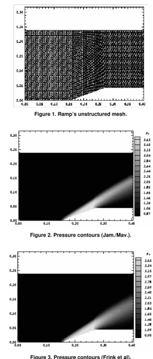
Mach number used in this simulation was 4,0, characterizing a supersonic flow. Figure 1 shows the unstructured mesh used for the discretized Euler equations. The ramp has an inclination angle of 20°.
Figures 2 and 3 show pressure contours obtained by both Jameson and Mavriplis explicit scheme (1986) and Frink, Parikh and Pirzadeh explicit scheme (1991), respectively. A CFL number of 2.1 was used for the Jameson and Mavriplis scheme (1986), while a CFL number of 1.1 was used for the Frink, Parikh and Pirzadeh one. The computational cost per iteration and per cell was 0.000135s obtained for the Jameson and Mavriplis scheme (1986), while Frink, Parikh and Pirzadeh scheme (1991) presented a computational cost of 0.000198s.
Figure 1. Ramp’s unstructured mesh.
Figure 2. Pressure contours (Jam./Mav.).
Figure 3. Pressure contours (Frink et al).
Jameson and Mavriplis scheme presents a peak of pressure grater than that obtained by Frink, Parikh and Pirzadeh scheme.
Pirzadeh scheme (1991), respectively. It is possible to note that Mach number contours in the Frink, Parikh and Pirzadeh scheme are smoother than that of the Jameson and Mavriplis scheme. It describes a more diffusive solution obtained for Frink, Parikh and Pirzadeh method because of its first order of accuracy in space. Such behaviour of generating excess of diffusion and loss of accuracy in the solution, associated with schemes of first-order spatial accuracy, is well known from literature: Harten (1983), Harten (1984), Sweby (1984) and Liou (1996)
Figure 4. Mach number contours (Jam./Mav.).
Figure 5. Mach number contours (Frink et al).
Figures 6 and 7 show density contours generated by Jameson and Mavriplis scheme (1986) and by Frink, Parikh and Pirzadeh scheme (1991), respectively.
Figure 6. Density contours (Jam./Mav.).
Figure 7. Density contours (Frink et al).
Figures 8 and 9 present pressure ratio distribution over the ramp studied here, obtained for the Jameson and Mavriplis (1986) and for the Frink, Parikh and Pirzadeh (1991) schemes, respectively. The pressure ratio distribution of the Frink, Parikh and Pirzadeh method presents constant pressure behaviour just after the shock wave; on the contrary, the Jameson and Mavriplis method presents a peak of pressure and a constant region just behind it. In this case, the solution described by Jameson and Mavriplis scheme is worse than that described by Frink, Parikh and Pirzadeh scheme. The better treatment of the flux vectors by the Frink, Parikh and Pirzadeh scheme becomes possible the establishment of the constant pressure region just after the shock wave.
Figure 8. Pr/Pr(free) distribution at wall (Jam./Mav.).
Figures 10 and 11 show convergence histories of each method obtained for this problem. The convergence rate of Jameson and Mavriplis scheme is better than that of Frink, Parikh and Pirzadeh scheme. The steady state solution obtained for the former was reached in 222 iterations. On the other hand, the steady state solution obtained for the latter was reached in 255 iterations. Both schemes present similar behaviour in terms of convergence rate for this problem.
Figure 10. Convergence history (Jam./Mav.).
Figure 11. Convergence history (Frink et al).
One way to verify whether the results are good is to calculate the β angle of the shock wave in relation to freestream direction. It is possible to determine from Figures 2 and 3 the shock angle of each numerical scheme. Making this measure, it is possible to encounter for the Jameson and Mavriplis scheme a shock angle of βJM = 33° and, repeating the same procedure, it is also possible to
encounter a shock angle of βFPP = 36° for the Frink, Parikh and
Pirzadeh. So in Anderson (1984) is possible to determine the β angle as function of the freestream Mach number and the angle of inclination of the ramp. For an angle of inclination of 20° and for the freestream Mach number of 4.0, it is possible to encounter an β angle of 32.5°. Hence, it is possible to verify that the Jameson and Mavriplis angle is in very good agreement with the shock angle.
Supersonic Flow Over a Blunt Body
An algebraic mesh with 7,056 triangular real volumes and 3,650 nodes was generated for the blunt body configuration. The far field was located at 25 times the blunt body nose’s ratio. Initial
conditions were set as freestream Mach number equals to 10.0, hypersonic flow, and the angle of attack equalled to 0.0°. A CFL number of 0.7 was used by the Jameson and Mavriplis scheme while a CFL number of 0.6 was used by the Frink, Parikh and Pirzadeh scheme. Figure 12 shows unstructured mesh used for this physical problem.
Figures 13 and 14 show pressure contours obtained by the Jameson and Mavriplis scheme and by the Frink, Parikh and Pirzadeh scheme, respectively. The Jameson and Mavriplis scheme presents a peak of pressure in front of the nose greater than that obtained for the Frink, Parikh and Pirzadeh scheme. This behaviour is due to the second order accuracy generated by the spatial discretization of the Jameson and Mavriplis scheme (1986), which permits more precise results.
Figure 12. Blunt Body’s unstructured mesh.
Figure 13. Pressure contours (Jam./Mav.).
Figures 15 and 16 present the Mach number contours generated by the Jameson and Mavriplis scheme (1986) and by the Frink, Parikh and Pirzadeh scheme (1991), respectively. Jameson and Mavriplis solution presents a peak of Mach number greater than that obtained by Frink, Parikh and Pirzadeh solution. The Frink, Parikh and Pirzadeh method underpredicts the Mach number distribution in the field in relation to Jameson and Mavriplis scheme.
Figure 15. Mach number contours (Jam./Mav.).
Figure 16. Mach number contours (Frink et al).
Figure 17. Density contours (Jam./Mav.).
Figure 18. Density contours (Frink et al).
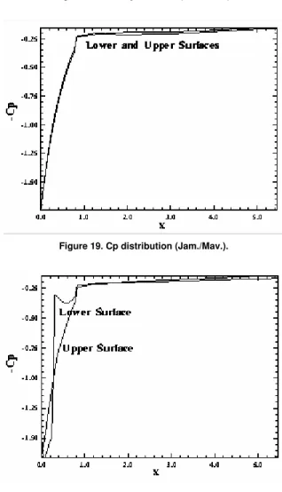
Figure 19. Cp distribution (Jam./Mav.).
Figure 20. Cp distribution (Frink et al).
Figures 17 and 18 present the density contours generated by the Jameson and Mavriplis scheme (1986) and by the Frink, Parikh and Pirzadeh scheme (1991), respectively. The density fields generated by both schemes are similar, although the peak of density is more highlighted by the Jameson and Mavriplis scheme.
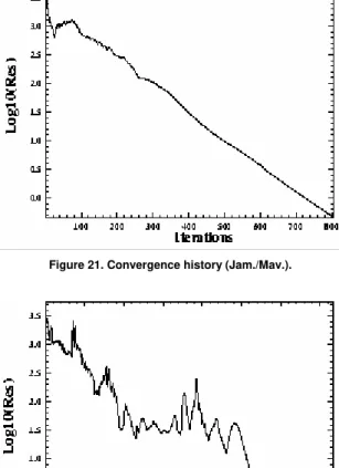
Figures 21 and 22 show the convergence history for Jameson and Mavriplis scheme (1986) and for the Frink, Parikh and Pirzadeh scheme (1991), respectively. The Jameson and Mavriplis scheme (1986) presents convergence in 805 iterations, while the Frink, Parikh and Pirzadeh scheme (1991) presents convergence in 1,831 iterations. For this problem, the Jameson and Mavriplis scheme has presented faster rate of convergence than that generated for the Frink, Parikh and Pirzadeh scheme.
Figure 21. Convergence history (Jam./Mav.).
Figure 22. Convergence history (Frink et al).
One possibility for quantitative comparison of both schemes is the determination of the stagnation pressure ahead of the configuration. Anderson (1984) presents a table of properties from normal shock waves in its B Appendix. This table permits the determination of some properties of shock waves as function of the freestream Mach number. In front of the configurations studied in this paper, the shock waves present a normal shock behaviour, which permits the determination of the stagnation pressure, after shock wave, from the tables encountered in Anderson (1984). So it is possible to determine de ratio pr0 pr∞ from Anderson (1984), where pr0 is the stagnation pressure in front of the configuration and
pr∞ is the freestream pressure (equals to 1/γ for the present nondimensionalization).
Hence, for this problem, M∞ = 10.0, pr0 pr∞= 129,2 and pr∞ =
0.714, permitting the determination of pr0 as equal to 92.25. Values
of pr0(JM) = 82.46 and pr0(FPP) = 78.65 are encountered from Figures
13 and 14, respectively. The relative errors were 10.6% for the Jameson and Mavriplis method and 14.7% for the Frink, Parikh and
Pirzadeh method. The Jameson and Mavriplis scheme was better than Frink, Parikh and Pirzadeh scheme for this problem.
Hypersonic Flow Over a Double Ellipsoid
An algebraic mesh with 8,232 triangular real volumes and 4,250 nodes was generated by the physical problem of the double ellipsoid. The far field was located at 5 times the major semi-axis of the greater ellipsoid. The unstructured mesh is shown in Figure 23. A CFL number of 0.2 was used by the Jameson and Mavriplis scheme, while a CFL number of 0.7 was used by the Frink, Parikh and Pirzadeh scheme. The initial condition used a freestream Mach number of 15.0 and zero attack angle.
Figure 23. Double Ellipsoid’s unstructured mesh.
Figure 24. Pressure contours (Jam./Mav.).
Figure 26. Mach number contours (Jam./Mav.).
Figure 27. Mach number contours (Frink et al).
Pressure contours of Jameson and Mavriplis scheme (1986) and Frink, Parikh and Pirzadeh scheme (1991) are exhibited in Figures 24 and 25, respectively. The pressure distribution of Frink, Parikh and Pirzadeh method is underpredicted. This has a result in the calculation of pressure and moment coefficients. These coefficients are essential for aerodynamic projects of aerospace vehicles.
Figures 26 and 27 show Mach number contours obtained for both schemes. The Jameson and Mavriplis method presents a peak of Mach number grater than the Frink, Parikh and Pirzadeh method. The Mach number field is underpredicted by the Frink, Parikh and Pirzadeh method. The excessive dissipative effect of the Frink, Parikh and Pirzadeh method because of its first order of spatial discretization is the main reason for that solution’s behaviour.
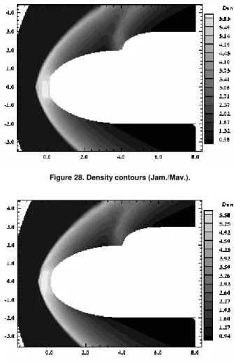
Figures 28 and 29 show the density contours for the Jameson and Mavriplis method and for Frink, Parikh and Pirzadeh method, respectively. Again, the density field is underpredicted by the Frink, Parikh and Pirzadeh scheme.
Figure 28. Density contours (Jam./Mav.).
Figure 29. Density contours (Frink et al).
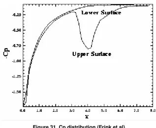
Figures 30 and 31 present the –Cp distribution over the lower and upper surfaces of the double ellipsoid for both schemes. The distribution of –Cp is more sharply defined for the Jameson and Mavriplis solution than for the Frink, Parikh and Pirzadeh solution.
Figure 31. Cp distribution (Frink et al).
Figures 32 and 33 show convergence histories described for the Jameson and Mavriplis method and for the Frink, Parikh and Pirzadeh method, respectively. The Jameson and Mavriplis method presents convergence in 4,380 iterations while the Frink, Parikh and Pirzadeh method presents convergence in 2,186 iterations. For this problem, the Frink, Parikh and Pirzadeh method has presented a rate of convergence greater than the Jameson and Mavriplis one.
Figure 32. Convergence history (Jam./Mav.).
Figure 33. Convergence history (Frink et al).
For this problem, M∞ = 15.0, it is possible to encounter in the B Appendix of Anderson (1984) the value of the ratio pr0 pr∞=
290.2. Hence for pr∞ = 0.714, the stagnation pressure in front of the double ellipsoid configuration is 207.20. The stagnation pressure calculated by the Jameson and Mavriplis scheme (1986) is 189.78 and the same pressure calculated by the Frink, Parikh and Pirzadeh scheme (1991) is 184.81, both pressures encountered in Figures 24 and 25, respectively. The relative errors for each scheme were 8.4% for the Jameson and Mavriplis scheme and 10.8% for the Frink, Parikh and Pirzadeh scheme. Again, the Frink, Parikh and Pirzadeh scheme was worse than the Jameson and Mavriplis scheme.
Supersonic Flow Over a Simplified Configuration of VLS
Figure 34. Simplified VLS’ unstructured mesh.
An algebraic mesh with 9,860 triangular real volumes and 5,130 nodes was generated by the physical problem of a supersonic flow over a simplified configuration of VLS. Figure 34 exhibits the generated unstructured mesh. The far field was located at 25 times the VLS nose’s ratio.
The initial condition used a freestream Mach number of 4.0 and 0.0° attack angle. The CFL number used by Jameson and Mavriplis scheme (1986) was 1.6, while the CFL number used by Frink, Parikh and Pirzadeh scheme (1991) was 0.5.
Figures 35 and 36 show pressure contours for the Jameson and Mavriplis scheme and for the Frink, Parikh and Pirzadeh scheme, respectively. It is possible to note that, for this problem, the Jameson and Mavriplis scheme underpredicts the pressure field in relation to Frink, Parikh and Pirzadeh one.
Figure 36. Pressure contours (Frink et al).
Figures 37 and 38 exhibit Mach numbers contours for the Jameson and Mavriplis scheme (1986) and for the Frink, Parikh and Pirzadeh scheme (1991), respectively. It is possible to note from these figures that the Mach number contours are more sharply defined by the Jameson and Mavriplis scheme, representing no excessive dissipation provided by this scheme.
Figure 37. Mach number contours (Jam./Mav.).
Figure 38. Mach number contours (Frink et al).
Figure 39. Density contours (Jam./Mav.).
Figure 40. Density contours (Frink et al).
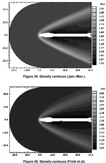
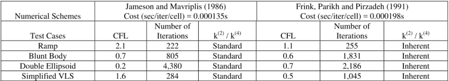
Figures 39 and 40 show the density contours generated for the Jameson and Mavriplis scheme (1986) and for the Frink, Parikh and Pirzadeh scheme (1991), respectively.
Figures 41 and 42 present the –Cp distribution over lower and upper surfaces of the simplified configuration of VLS. Both schemes have presented similar behaviour.
Figure 42. Cp distribution (Frink et al).
Figure 43. Convergence history (Jam./Mav.).
Figure 44. Convergence history (Frink et al).
Figures 43 and 44 exhibit the convergence histories for both schemes. The Jameson and Mavriplis scheme (1986) has reached a steady state condition in 284 iterations, while the Frink, Parikh and Pirzadeh scheme (1991) has reached a steady state condition in 1,045 iterations. So, the Jameson and Mavriplis scheme presented a better convergence rate than the Frink, Parikh and Pirzadeh scheme (3.7 times faster).
For this problem, M∞ = 4.0, it is possible to encounter in Anderson (1984) the value of the ratio pr0 pr∞ = 21.07. Hence, for pr∞ = 0.714, the stagnation pressure in front of the simplified configuration of VLS is 15.04. The stagnation pressure calculated by the Jameson and Mavriplis scheme (1986) is 6.81 and the same pressure calculated by the Frink, Parikh and Pirzadeh scheme (1991) is 10.16, both pressures encountered in Figures 35 and 36, respectively. The relative errors for each scheme were 54.7% for Jameson and Mavriplis scheme and 32.4% for Frink, Parikh and Pirzadeh scheme. In this case, the Frink, Parikh and Pirzadeh scheme was better than the Jameson and Mavriplis scheme.
Table 1 presents a summary of the overall computational results obtained for Jameson and Mavriplis (1986) and Frink, Parikh and Pirzadeh (1991) schemes.
Table 1. Computational Performance of Jameson and Mavriplis and Frink, Parikh and Pirzadeh Schemes.
Numerical Schemes
Jameson and Mavriplis (1986) Cost (sec/iter/cell) = 0.000135s
Frink, Parikh and Pirzadeh (1991) Cost (sec/iter/cell) = 0.000198s
Test Cases CFL
Number of
Iterations k(2) / k(4) CFL
Number of
Iterations k(2) / k(4)
Ramp 2.1 222 Standard 1.1 255 Inherent
Blunt Body 0.7 805 Standard 0.6 1,831 Inherent
Double Ellipsoid 0.2 4,380 Standard 0.7 2,186 Inherent
Simplified VLS 1.6 284 Standard 0.5 1,045 Inherent
As can be seen in this table, the Jameson and Mavriplis scheme (1986) is better than Frink, Parikh and Pirzadeh scheme (1991). Only for the problem of the double ellipsoid, Frink, Parikh and Pirzadeh algorithm presents a higher rate of convergence than Jameson and Mavriplis algorithm. Even so, the qualitative and quantitative results to the double ellipsoid problem for the Jameson and Mavriplis scheme were better than those for the Frink, Parikh and Pirzadeh scheme. The Frink, Parikh and Pirzadeh scheme presents better quantitative results for the simplified configuration of VLS than the Jameson and Mavriplis scheme. Both schemes present similar behaviour of robustness: every problems were tested and results were compared, resulting in good features of robustness for both schemes. The computational cost were very similar for the
schemes tested, which represents a good feature of the Frink, Parikh and Pirzadeh algorithm.
Conclusions
performance, some aspects of solution quality and robustness were studied, showing advantages and disadvantages between the two algorithms.
In general aspects, the Jameson and Mavriplis scheme (1986) is better than the Frink, Parikh and Pirzadeh scheme (1991) in terms of high rate of convergence and run time for the aeronautical problems studied. The computational cost of the Frink, Parikh and Pirzadeh scheme (1991) is worse than Jameson and Mavriplis scheme (1986). General aspects of solution quality and robustness for the Frink, Parikh and Pirzadeh scheme (1991) are not so different of those respective features of the Jameson and Mavriplis scheme (1986). The Frink, Parikh and Pirzadeh method (1991) has presented the same robustness features of the Jameson and Mavriplis method (1986), mainly, for the hypersonic “cold gas” examples tested herein. Hence, the Jameson and Mavriplis scheme (1986) was more efficient than the Frink, Parikh and Pirzadeh scheme (1991) for the high speed aerospace problems studied.
References
Anderson, J. D., Jr., 1984, “Fundamentals of Aerodynamics”, McGraw-Hill, Inc., EUA, 563p.
Arnone, A., Liou, M. -S., and Povinelli, L. A., 1991, “Multigrid Calculation of Three-Dimensional Viscous Cascade Flows”, AIAA Paper 91-3238-CP.
Azevedo, J. L. F., 1992, “A Finite Difference Method Applied to Internal Axisymmetric Flows”, Bulletin of Brazilian Society of Applied and Computational Mathematics, Vol. 3, No. 1, Series II, pp. 1-20.
Batina, J. T., 1990, “Unsteady Euler Airfoil Solutions Using Unstructured Dynamic Meshes”, AIAA Journal, Vol. 28, No. 8, pp. 1381-1388.
Frink, N. T., Parikh, P., and Pirzadeh, S., 1991, “Aerodynamic Analysis of Complex Configurations Using Unstructured Grids”, AIAA 91-3292-CP.
Frink, N. T., 1992, “Upwind Scheme for Solving the Euler Equations on Unstructured Tetrahedral Meshes”, AIAA Journal, Vol. 30, No. 1, pp. 70-77.
Harten, A., 1983, “High Resolution Schemes for Hyperbolic Conservation Laws”, Journal of Computational Physics, Vol. 49, pp. 357-393.
Harten, A., 1984, “On a Class of High Resolution Total-Variation-Stable Finite-Difference Schemes”, SIAM J. Numerical Analysis, Vol. 21, No. 1, pp. 1-23.
Hefazi, H. and Chen, L. T., 1992, “A Composite Structured/Unstructured-Mesh Euler Method for Complex Airfoil Shapes”, Proceedings of 5th Symposium on Numerical and Physical Aspects of Aerodynamic Flow, Long Beach, California, US, Section 4, pp. 1-6.
Hooker, J. R., Batina, J. T., and Williams, M. H., 1992, “Spatial and Temporal Adaptive Procedures for the Unsteady Aerodynamic Analysis of Airfoils Using Unstructured Meshes”, AIAA Paper 92-2694-CP.
Jameson, A., and Mavriplis, D. J., 1986, “Finite Volume Solution of the Two-Dimensional Euler Equations on a Regular Triangular Mesh”, AIAA Journal, Vol. 24, No. 4, pp. 611-618.
Jameson, A., Schmidt, W., and Turkel, E., 1981, “Numerical Solution of the Euler Equations by Finite Volume Methods Using Runge-Kutta Time Stepping Schemes”, AIAA Paper 81-1259.
Korzenowski, H., and Azevedo, J. L. F., 1996, “Geração de Malhas Não-Estruturadas para Aplicação em Mecânica dos Fluidos”, Proceedings of the 4th Congress of Mechanical Engineering - North/Northeast, Recife, PE, Brazil, pp. 779-783.
Liou, M. -S., 1996, “A Sequel to AUSM: AUSM+”, Journal of Computational Physics, Vol. 129, pp. 364-382.
Long, L. N., Khan, M. N. S., and Sharp, H. T., 1991, “Massively Parallel Three-Dimensional Euler / Navier-Stokes Method”, AIAA Journal, Vol. 29, No. 5, pp. 657-666.
Luo, H., Baum, J. D., and Löhner, R., 1994, “Edge-Based Finite Element Scheme for the Euler Equations”, AIAA Journal, Vol. 32, No. 6, pp. 1183-1190.
Maciel, E. S. G., and Azevedo, J. L. F., 1997, “Comparação entre Vários Algoritmos de Fatoração Aproximada na Solução das Equações de Navier-Stokes”, Proceedings of the 14th Brazilian Congress of Mechanical Engineering (available in CD-ROM), Bauru, SP, Brazil.
Maciel, E. S. G., and Azevedo, J. L. F., 1998, “Comparação entre Vários Esquemas Implicitos de Fatoração Aproximada na Solução das Equações de Navier-Stokes”, RBCM- Journal of the Brazilian Society of Mechanical Sciences, Vol. XX, No. 3, pp. 353-380.
Maciel, E. S. G., and Azevedo, J. L. F., 2001, “Solution of Aerospace Problems Using Structured and Unstructured Strategies”, RBCM- Journal of the Brazilian Society of Mechanical Sciences, Vol. XXIII, No. 2, pp. 155-178.
Mavriplis, D. J., and Jameson, A., 1987, “Multigrid Solution of the Euler Equations on Unstructured and Adaptive Meshes”, ICASE Report No. 87-53.
Mavriplis, D. J., 1990, “Accurate Multigrid Solution of the Euler Equations on Unstructured and Adaptive Meshes”, AIAA Journal, Vol. 28, No. 2, pp. 213-221.
Mavriplis, D. J., 1995, “An Advancing Front Delaunay Triangulation Algorithm Designed for Robustness”, Journal of Computational Physics, Vol. 117, pp. 90-101.
Pirzadeh, S., 1991, “Structured Background Grids for Generation of Unstructured Grids by Advancing Front Method”, AIAA Paper 91-3233-CP.
Roe, P. L., 1981, “Approximate Riemann Solvers, Parameter Vectors, and Difference Schemes”, Journal of Computational Physics, Vol. 43, pp. 357-372.
Roe, P. L., 1986, “Characteristic Based Schemes for the Euler Equations”, Annual Review of Fluid Mechanics, Vol. 18, pp. 337-365.
Swanson, R. C., and Radespiel, R., 1991, “Cell Centered and Cell Vertex Multigrid Schemes for the Navier-Stokes Equations", AIAA Journal, Vol. 29, No. 5, pp. 697-703.