Sba Controle & Automação vol.22 número6

APPLYING GLOBAL TIME PETRI NET ANALYSIS ON THE EMBEDDED

SOFTWARE CONTEXT

Leticia Mara Peres

Luis Allan K ¨unzle

Eduardo Todt

∗_{Departamento de Inform´atica}

Universidade Federal do Paran´a Curitiba, Paran´a, Brasil

RESUMO

Aplicac¸˜ao da An´alise Global de Redes de Petri Temporais no Contexto de Software Embarcado

Redes de Petri e suas propriedades alg´ebricas s˜ao usadas para modelar e analisar sistemas envolvendo paralelismo, concorrˆencia e sincronizac¸˜ao. Este artigo apresenta uma aplicac¸˜ao da t´ecnica de Tempo Global (GTT - global time

te-chnique) que ´e uma abordagem para construir grafos de

clas-ses de redes de Petri temporais baseada nos tempos relativo e global. Al´em da construc¸˜ao deste grafo de classes propomos uma an´alise de escalonabilidade do tipo temporal quantita-tiva para pol´ıticas de prioridade fixa e earliest deadline first (EDF). Propomos que a an´alise de cen´arios, ou a durac¸˜ao de itiner´arios de comportamento, de um sistema pode ser feita usando esta t´ecnica.

PALAVRAS-CHAVE: Rede de Petri Temporal, An´alise Quan-titativa, Software Embarcado.

ABSTRACT

This paper presents an application of Global Time technique (GTT) which is an approach to construct class graphs of Time Petri nets based on relative and global time. Besides the constructing of GTT class graph we propose a schedulability

Artigo submetido em 10/03/2011 (Id.: 01294) Revisado em 11/05/2011, 15/07/2011, 15/08/2011

Aceito sob recomendac¸ ˜ao do Editor Associado Prof. Carlos Roberto Minussi

analysis of quantitative time type for fixed priority policies and Earliest Deadline First (EDF). We propose that analysis of scenarios, or behavior itineraries duration of a system, can be done using this approach.

KEYWORDS: Time Petri Net, Quantitative Analysis, Em-bedded Software.

1

INTRODUCTION

Petri nets (PN) (Murata, 1989) and their algebraic properties are used to model and analyze systems involving parallelism, concurrency and synchronization. Several extensions of ba-sic formalism have been proposed in order to increase their modeling capacity. In this work we are interested in Time Petri nets (TPN), where quantitative time restrictions can be considered (Merlin, 1974).

systems. They present a set of PN design patterns to model tasks with preemptive scheduling and provide a method using a polyhedron representation and later difference bound ma-trix. Yet, they describe observers that give a numeric result for the computation of response times of tasks. In (Lime and Roux, 2008), the authors use their scheduling TPN design patterns of (Lime and Roux, 2003) to model tasks and deal with Fixed Priority and Earliest Deadline First policies, with the possibility of using round-robin for tasks with the same priority. In (Cortes et al., 2000) and (Lime and Roux, 2008) the nets are translated into linear hybrid automata and timed properties are verified using the symbolic model checking Hytech tool (Henzinger et al., 1997).

The prevalent technique in the literature of TPN analy-sis is based on the graph of state classes (Berthomieu and Menasche, 1983), (Berthomieu and Diaz, 1991) and (Berthomieu and Vernadat, 2003). This is an enumerative method which generates a reachable state space using the behavior of a TPN. In this method, each class is a graph node and groups the state set with the same marking, and each time interval encompasses possible firing instants for each enabled transition in the class. Each enabled transition can fire in each class once, generating another class, and this possible firing is an arc graph linking these two classes. This method finds the relative time interval during which the sys-tem remains in a particular class.

Wang et al. at (Wang et al., 2000), propose to find the TPN global time using a class graph based on (Berthomieu and Menasche, 1982). The global time corresponds to absolute time of the accumulation of time since the beginning of net execution, or initial marking, until the observed class, i.e., referring time information to the chaining of events repre-sented by transitions firing sequences. In this method, the unique time is calculated with no adjustments for concurrent enabled transitions.

In this paper we propose an application of the Global Time Technique (GTT). GTT was proposed by Lima et al. in (Lima et al., 2005), (Lima et al., 2006), and (Lima et al., 2008), and is an extension of (Berthomieu and Menasche, 1982) and (Wang et al., 2000) methods, and generates a TPN class graph with two types of time that are useful and usable in a Petri net simulation: relative and global time. The nov-elty of the work presented in this paper is propose an algo-rithm that handles a k-limited TPN and an application which makes possible verify the schedulability of real-time embed-ded software. A k-limited TPN is one that its places can contain at mostktokens,k≥1. GTT computes global time information using relative time intervals of (Berthomieu and Menasche, 1982) and adjusting the obtained time consider-ing the persistence or not of enabled transitions. GTT han-dles concurrent events reducing the increase of imprecision

when compared to the simple sum of relative times, due to adjustments of this technique. The global time information is correct for both limits of time interval of any class, even when the net represents concurrency among events (Lima et al., 2006), (Lima et al., 2008) e (Mattar Junior et al., 2007).

This paper is a revised and extended version of a work pub-lished in Portuguese at XVIII Congresso Brasileiro de Au-tom´atica (CBA2010) proceedings (Peres et al., 2010). It con-cerns the application of global time TPN on the embedded software context and is a result of studies about TPN analysis using interval algebra initiated by (Lima et al., 2005), (Lima et al., 2006), and (Lima et al., 2008). We use some proce-dures and calculations defined by (Mattar Junior et al., 2007) which presented studies about firing sequence global time analysis of 1-limited TPN.

The remainder of this paper is organized as follows. Sec-tion 2 defines basic concepts of interval operaSec-tions, TPN and class graph. Section 3 establishes GTT, gives an algorithm for computing the GTT class graph, and presents an example of its application. Section 4 presents an application of GTT on the context of embedded software verification, while Sec-tion 5 concludes the article.

2

BASIC CONCEPTS

The Global Time Technique (GTT) is a TPN analysis based on operations on numeric intervals. In this section we define the basic concepts used by GTT.

2.1

Numeric Intervals

Definition 1 (Intervals and Operations) Given two rational

numbers,aandb, such thata≤b. We denote[a, b]as the set

{x ∈Q : a≤ x≤b}, defined as a closed interval froma tob. An interval[c, d]is denoted as not proper whend < c, withcanddrationals.

Leta, b, canddbe rational numbers, given the intervals[a, b]

and[c, d], proper or not proper, we define the following op-erations:

[a, b] + [c, d] = [a+c, b+d]

[a, b]−[c, d] = [max{0, a−d}, max{0, b−c}] [a, b]⊖[c, d] = [max{0, a−c}, max{0, b−d}]

2.2

Time Petri nets

Definition 2 (Time Petri Net) A time Petri net is a tuple

T P N = (P, T, P re, P os, e)(Berthomieu and Diaz, 1991), where:

• Pis a finite set of places,P 6=∅,

• Tis a finite set of transitions,T 6=∅,

• P reis an weight function of arcs from places to transi-tions,P re: (P×T)→N,

• P osis an weight function of arcs from transitions to places,P os: (T×P)→N,

• M0is the initial marking, and

• e : T → (Q+_×

(Q+_{∪ {∞}}

))such ase(t) = [a, b], wheret∈Tand[a, b]is an interval.

A marking is an assignment of tokens to places that defines the state of the net. The marking of a placep∈Pis denoted M(p), such asM :P →N. The initial marking of a TPN is denoted byM0.

Definition 3 (Enabled transition) A transitiont ∈ T is en-abled in a markingMkiff for allp∈P,Mk(p)≥P re(p, t).

Definition 4 (Firing) Iftis an enabled transition in a mark-ingMk₋1, thentcan fire. The firing oft changes de state

of the net and produces a new marking. The new marking Mkis given byMk(p) =Mk₋1(p)−P re(p, t) +P os(t, p),

for allp∈P. The firing oftis denoted byMk₋1[tiMk. If

the firing oftis succeeded by one or more transition firings, we say that this sequence of firings form a firing sequences. The firing ofsin a markingMjproduces a sequence of new

markings ended byMk, denoted byMj[siMk.

A TPN has one static time intervale(t) = [a, b], witha≤b, associated to each transitiont ∈T. The limitsaandb rep-resent, respectively, the earliest and the latest possible firing time of transitiont, counted from the instant whent is en-abled.

Definition 5 (State class) A state class of a TPN is a tuple

ck = (Mk, Wk), whereMk is the marking that defines de

state of the net andWk is the time information set

associ-ated with this marking. Wk will be further detailed in the

Definition 14.

We say that a transitiont ∈ T is enabled (fires) in a class ck ifftis enabled (fires) inMk. When a transitiontfires in

a certain classck−1, at levelk−1, the TPN reaches a new

marking and a new classckat levelk.

Definition 6 (State class graph) The state class graph is a

directed graphS = (C, A)where each nodec∈Cis a state class and each arca ∈ Aconnects one class ck₋1, at level

k−1, to an immediately succeeding class ck. Each arc is

labeled with one transitiont∈T which is fired inck₋1. The

root node of the class graph is the start classc0, that has the

initial markingM0.

The firing oftalso produces a new classck in the graphS

from the classck₋1and is denoted byck₋1[tick. We say that

classck₋1is immediately preceding tock.

One firing sequencesis reflected in the class graphS. The succeeded firing of one or more transitions in a TPN, from a classck to another classck+n, is represented byck[sick₋n,

wheren≥0is the sequence size.

Definition 7 (Newly enabled transition) A transitiont∈T, enabled in a certain classck, is a newly enabled transition in

ckiftsatisfies one of following:

• twas not enabled in classck−1; or

• the firing oft originated the classck, that is,tfired in

the classck₋1and it was re-enabled inck.

Definition 8 (Persistent transition) A transitiont ∈ T, en-abled in a certain classck, is a persistent transition inckift

was enabled in a classck₋1, immediately preceding tockand

tdid not fired inck₋1. Persistent is equivalent to not newly

enabled.

3

GLOBAL TIME TECHNIQUE

Particularly for the Global time technique (GTT), the infor-mation set Wk of classck has, for each enabled transition,

two types of time information: relative and global. Rela-tive time information refers to the accumulated time since the transition had been enabled until reaches the classck. Global

time information refers to the accumulated time since the ini-tial marking, or start class c0, until ck (Lima et al., 2005).

Firstly in this section we define GTT elements which com-pound relative and global time information and then we re-define the state class and the class graph. We present also an algorithm to generate GTT state class graph for a k-limited TPN and definitions of computing total time for a firing se-quence and the permanence time in a state.

Definition 9 (Relative time interval) Letrk(ti)be the

rela-tive time interval of a transition ti calculated in a class ck

such thatck₋1[tfick, defined as:

rk(ti) =

e(ti) case 1,

where cases 1 and 2 are, respectively:

1. tiis newly enabled inck;

2. tiis persistent inck.

The relative time intervalrk(ti)of the enabled transitionti

of a classck is used to identify which transitions are firable

at classck.

Definition 10 (Firable transition) A transition tf with

rk(tf) = [af, bf]is firable inck ifftf is enabled inck and

there is no other transitiontiwithrk(ti) = [ai, bi]enabled

incksuch thatbi< af.

Definition 11 (Persistence coefficient) A persistence

adjust-ment coefficientack(ti)of an enabled transitiontiin a class

cksuch thatck₋1[tfick, is defined as:

ack(ti) =



  

  

rk−1(ti)⊖rk−1(tf) case 1,

ack−1(ti)⊖rk−1(tf) case 2,

rk₋1(ti)⊖ack₋1(tf) case 3,

ack₋1(ti)⊖ack₋1(tf) case 4,

where cases 1 to 4 are respectively:

1. tiandtfare both newly enabled inck−1;

2. tiis persistent andtf is newly enabled, both inck₋1;

3. tiis newly enabled andtfis persistent, both inck−1;

4. tiandtfare both persistent inck−1.

The persistence adjustment coefficientack(ti)is used to

ad-just the computing of global time and prevents the increase of imprecision, as proved by (Mattar Junior et al., 2007).

Definition 12 (Global time interval) A global time interval

gk(ti)of firing of a firable transitiontiin a classcksuch that

ck−1[tfickis:

gk(ti) =







e(ti) case 1,

gk−1(tf) +rk(ti) case 2,

gk−1(tf) +ack(ti) case 3,

where cases 1 to 3 are respectively:

1. k= 0;

2. k6= 0andtiis newly enabled inck;

3. k6= 0andtiis persistent inck.

The global time intervalgk(tf)of firing of a transitiontf in

a classckis a time interval counted from the initial marking

until the firing instant oftf in the classck.

However, in order to take a conservative character, supposing the firing of all firable transitions, it is necessary to adjust the interval upper bound ofgk(ti).

Definition 13 (Upper bound adjustment) Lettfbe the fired

transition in a class ck such that ck[tfick+1. The upper

bound of global time intervalgk(tf) = [af, bf]of the fired

transitiontf, must be adjusted by the lowest upper bound of

intervals calculated to alltiin the classck, generating a new

gk(tf), such as:

gk(tf) = [af, b],

whereb=min{bi|gk(ti) = [ai, bi], ∀tifirable inck}.

Definition 14 (GTT state class) A GTT state class ck

of a T P N, is a tuple ck = (Mk, Wk), with Wk =

(H, E, F, R, G), where:

• Mkis the marking ofck;

• His the enabled transition set inck;

• Eis one tuplehE0, E1, E2iwhich contains persistence

information of transitions of classck where: E0is the

set of newly enabled transition inck, E1 is the set of

persistent transitions inck that was newly enabled in

ck₋1, andE2 is the set of persistent transition in the

classesckthat was also persistent inck₋1;

• Fis the firable transition set inck;

• Ris the relative domain set which contains relative time intervalsrk(ti)of all enabled transitionstiinck.

• Gis one tuplehack, gkiwhich corresponds to the global

time domain ofck, whereack(ti)is the persistence

ad-justment coefficient of all persistent transitionstiinck

andgk(tj)is the global time interval of all firable

tran-sitionstjinck.

Definition 15 (GTT state class graph) The GTT state class

graph is a state class graph where each node is a GTT state

class and each arc is labeled with one fired transition, as in

the Definition 6.

3.1

The class graph algorithm

3.1.1 The input data

• The net structure, represented by one input incidence matrixpre= [P re(p, t), p∈P, t∈T]and one output incidence matrixpos= [P os(t, p), p∈P, t∈T];

• The static time informatione(t), for all t ∈ T, repre-sented by one arrayewith size|T|;

• The initial marking of the net represented by one array M0with size|P|.

3.1.2 The body

0) definek= 0;

Starting construction of classck:

1) determine the net markingMk: ifk = 0,Mk ← M0;

elseMkis already determined by the firing of transition

tf at step 7 from previous cycle;

2) determine the setHof enabled transitionstifromMk,

according to the Definition 3;

3) determine thehE0, E1, E2ituple, according to the

Def-inition 14;

4) compute the setRof relative time intervalsrk(ti)∀ti∈

H, according to the Definition 9;

5) determine the setF of firable transitionsticomparing

elements inR, according to the Definition 10;

6) determine theG tuple, computing: a) ack(ti), ∀ti ∈

{E1∪E2}, according to the Definition 11; and b)gk(ti),

∀ti∈F, according to the Definition 12;

Firing of allti∈F of classck:

7) ∀ti ∈ F execute all following steps: a) adjust interval

gk(ti), according to the Definition 13 being tf = ti

; b) create one successor classc with levelk+ 1and one arc connecting the classck with the new successor

classck+1, and label the arc withti; c) update the new

markingMk+1for the TPN, according to the Definition

4; and d) for all new successor classes with levelk+ 1, assign the new global timegk+1=gk(ti);

8) increasek←k+ 1and∀ti ∈F:tf ←tiand execute

steps 1 to 8;

3.1.3 The end

The algorithm is executed until all firable transitions in all classes have been fired.

3.2

Global time for a firing sequence

The global time of a firing sequencesofc0[sick, according

to the Definition 4, is obtained during construction of GTT class graph and is the resulting global time intervalgk₋1(tf),

being tf the last transition fired to reach class ck, that is,

ck₋1[tfick.

3.3

Permanence time in a class

The permanence time in a class refers to the minimum and maximum time that the system, represented by the TPN, re-mains in the state represented by the class.

Definition 16 (Permanence time in a class) We consider that

the firing of all firable transitions are mandatory, i.e., each firable transition must be fired until its upper bound of time interval has reached. The permanence time of a net in a cer-tain reachable classckis given by:

icck = [a, b]

where a = min{ai | rk(ti) = [ai, bi]} and b =

min{bi|rk(ti) = [ai, bi]},∀tifirable inck.

4

APPLICATION

4.1

Mapping between system tasks and

TPN

Given, according to (Lime and Roux, 2008) and definitions of section 2:

• τ ∈ Tasks, being Tasks the set of tasks of the embed-ded system, where there is no task migration between processors.

• Sched:Procs 7→ {FP,EDF} maps a processor to a scheduling policy, being FP “Fixed Priority” and EDF “Earliest Deadline First” ;

• Π: Tasks7→Procs maps a task to its processor;

• ̟: Tasks7→ N, for Sched(Π(τ)) = F P, gives the priority of the task on the processor;

• δ: Tasks7→(Q+_×

(Q+_{∪ {∞}}

)), forSched(Π(τ)) =

EDF, gives the deadline interval of the task relative to its activation time;

• γ : P 7→Tasks∪{φ}maps each place of the TPN to a task, whereφdenotes that the place is not mapped to any real task.

For each transitiont ∈ T, there is at most one placepsuch thatp∈P re(t)andγ(p)6=φ. If∀p∈ P re(t),γ(p) =φ, thentis not related to any real task andtis part ofφ, denoted byγ(t) =φ. Otherwise, for each transitiont,tis part of the

taskτ, denotedt∈τ, if one of its input places is mapped to τ :t ∈τ ⇔ ∃p∈P re(t), such thatγ(p) =τ. So,γ(t)is the task such thatt∈τ(Lime and Roux, 2008).

Each taskτ is modeled by a subnet of the TPN composed of places mapped toτbyγand transitionstwith static time e(t), which are parts of τ. At most one instance of each task is active at a given instant, which is expressed by the restriction that at most one place mapped toτbyγis marked at a given instant (Lime and Roux, 2008).

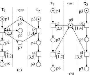
At Figures 1, 2 and 3 we present examples of design pat-terns to illustrate how Petri nets are modeled. These figures present some synchronization service modeling of embedded software tasks and are 1-limited Petri nets. These examples are shown just to illustrate the possibility of application of real time scheduling policies using TPN. More details can be found in (Lime and Roux, 2003).

We propose, after the TPN modeling, to generate a GTT state class graph, as presented at section 3.

τ

τ

p1

p2

t1

[2,3]

t2

[1,2]

p3

[1,4]

t3

p4

[3,5]

t4

Figure 1: TPN with two concurrent tasks on one processor (Lime and Roux, 2003).

t1 [1,2] p1

τ

(c)

τ

[1,1] t0

(b)

p2

p1

p3 t1 [1,2] p0

τ

(a)

[3,3] t0

p2 t1 [1,2] p1

Figure 2: TPN of activation schemata: (a) periodic activa-tion schema, (b) delayed periodic activaactiva-tion schema, and (c) cyclic activation schema (Lime and Roux, 2003).

4.2

Mapping between scheduling policies

and the GTT graph

τ

τ

τ

τ

1 sync 2

sync

(a)

(b) p1

p4

p9 p8

p5

p2

p1

p4

p7 t4

[3,5] t2

[1,2]

t3 [1,4] [2,3]t1

p7 p6

p3

t1 [2,3]

p2

t2 [1,2]

p6

t4 [3,5] t3 [1,4] p5

p3

Figure 3: TPN of synchronization: (a) model for memo-rized events and (b) model for shared resources using a semaphore (based on Lime and Roux, 2003).

We have established scheduling policy based criteria using “Earliest Deadline First” and “Fixed Priority” scheduling policies. For Sched:Procs 7→ {CE}, where CE is “Cyclic Executive”, the TPN model represents only one task which is typically realized as an infinite loop in main()(Lime and Roux, 2003), as shown in the Figure 2(c). Because CE has not a specific criterion in order to be satisfied, this policy is achieved only by modeling TPN and it is not necessary to formalize this function in relation to the path generation of the GTT state class graph.

4.2.1 Fixed Priority (Sched(Π(γ(t))) =F P)

The function̟: Tasks7→Nguides the enumeration of firing sequence. The firing sequence consists of firable transitions tf and the priorities of task executions associated to

transi-tionstiand, for the function̟,tf =ti, for alltiwith highest

priority. In the case of tasks with the same priority at some point, one of these criterion can guide the enumeration of the firing sequence among the processes with the same priority: a FIFO choice; an earliest deadline first considering the static timee(ti)for each transitionti, as we present in the

follow-ing section; or a random choice.

At the end of this enumeration, we already have the total time for a complete or partial firing sequence according to GTT, as presented in 3.2.

4.2.2 Earliest Deadline First (Sched(Π(γ(t))) =EDF)

Another type of firing sequence can be enumerated on class graph, using the Earliest Deadline First scheduling policy.

Then, the functionδ: Tasks7→(Q+_×(Q+_{∪ {∞}))guides}

this enumeration. Our criterion is to choose the transition which has the lowest deadline given byδ(τ)as following.

Letδ(τ)of a transitionti calculated in a classck such that

ck−1[tf > ck, and defined as: δ(τ) = LF T(rk(ti)). The

latest firing time (LFT) of the timerk(ti)for each transition

tiis the guide for firing sequence enumeration.

As the FP policy, at the end of enumeration already has the total time for a firing sequence, as presented in 3.2.

4.3

Examples

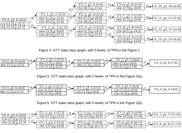
The Figures 4, 5, 6, and 7 refer to GTT state class graph of the Figures 1, 2(a), 2(b), and 3(b), respectively. The format of GTT state class graph presented in the Figures 4, 5, 6, and 7 is: each node is a rectangle and represents one classck∈C.

Each arc is a transition fired in the class ck and generated

the successor class ck+1. Each node has a data header and

lines with some elements of tupleWk. The header has the

following data, separeted by colons: the class name in the formatCk n, wherekis the level andnis a class identifier, and the class global time in the formatgk n, wherekis the level andnis a class identifier. The next lines of node present the time information of all enabled transition ti: the name

of transition ti; its relative timerk(ti); and its global time

gk(ti). Each arc is labeled with one fired transition which is

firable in the classck. In this article, our graphs are generated

until the fifth level of classes.

Considering the TPN of the Figure 1. The task τ1has

pri-ority ̟ = 1 and one preemption point. The task τ2 has

also one preemption point, but priority ̟ = 2. Then, ̟(t1) = 1, ̟(t2) = 1, ̟(t3) = 2 and̟(t4) = 2. The

TPN class graph according to GTT is presented in the Fig-ure 4. For Sched(Π(τ)) = F P, the firing sequence is: t3, t1, t4, t2. It is interesting to note that, according to the

Definition 10, t1 is the only one firable in the classC1 2,

even t4 being enable. The global time of this sequence is

g4 12 = [4,5]. ForSched(Π(τ)) = EDF, the firing

se-quence can bet1, t2, t3, t4, with global timeg4 10 = [6,9],

ort1, t3, t2, t4, with global timeg4 11= [5,9].

In the Figure 2(a), the TPN represents one task τ1 has

pri-ority̟ = 3and̟(t0) = 3,̟(t1) = 3. The

correspond-ing GTT graph is presented in the Figure 5. There is one possible firing sequence, for bothSched(Π(τ)) =F P and Sched(Π(τ)) = EDF, because in the classes C1 1 and C3 3onlyt1is firable whent0andt1are enabled.

The same considerations of the previous example can be made about the Figure 2(b): the TPN represents one taskτ1

corre-C0_0, g0_0=[0,0] t1)r=[2,3],g=[2,3] t3)r=[1,4],g=[1,3]

t1

t3

t3)r=[0,2],g=[2,4] C1_1, g1_1=[2,3] t2)r=[1,2],g=[3,4]

C1_2, g1_2=[1,3] t4)r=[3,5],g=[0,0] t1)r=[0,2],g=[2,3]

t2

t3

t1

t3)r=[0,1],g=[3,4]

t4)r=[3,5],g=[0,0] t2)r=[0,2],g=[3,5]

t4)r=[1,5],g=[4,5] t2)r=[1,2],g=[3,5] C2_3, g2_3=[3,4]

C2_4, g2_4=[2,4]

C2_5, g2_5=[2,3] t3

t2

t4

t2

t4

t4

t2

t4 t4)r=[3,5],g=[6,9]

t4)r=[1,5],g=[5,9]

t2)r=[0,1],g=[4,5]

t4)r=[0,4],g=[4,8] C3_6, g3_6=[3,4]

C3_7, g3_7=[3,5]

C3_8, g3_8=[4,5]

C3_9, g3_9=[3,5]

C4_10, g4_10=[6,9]

C4_11, g4_11=[5,9]

C4_12, g4_12=[4,5]

C4_13, g4_13=[4,8]

Figure 4: GTT state class graph, with 5 levels, of TPN in the Figure 1.

t0 C0_0, g0_0=[0,0] t0)r=[3,3],g=[3,3]

t1 t0)t=[3,3],g=[0,0] t1)r=[1,2],g=[4,5] C1_1, g1_1=[3,3]

t0)r=[1,2],g=[6,6]

C2_2, g2_2=[4,5] t0 _{t0)r=[3,3],g=[0,0]}C3_3, g3_3=[6,6] t1

t1)r=[1,2],g=[7,8]

C4_4, g4_4=[7,8]

Figure 5: GTT state class graph, with 5 levels, of TPN in the Figure 2(a).

C4_4, g4_4=[5,6] t1

t1)r=[1,2],g=[5,6] t2)r=[3,3],g=[0,0] t2)r=[1,2],g=[4,4]

t1)r=[1,2],g=[2,3] t2)r=[3,3],g=[0,0] t0)r=[1,1],g=[1,1]

C0_0, g0_0=[0,0] t0 C1_1, g1_1=[1,1] t1 _{C2_2, g2_2=[2,3]} t2 C3_3, g3_3=[4,4]

Figure 6: GTT state class graph, with 5 levels, of TPN in the Figure 2(b).

C0_0, g0_0=[0,0] t1)r=[2,3],g=[2,3] t3)r=[1,4],g=[1,3]

t2)r=[1,2],g=[3,5]

C1_2, g1_2=[1,3] t4)r=[3,5],g=[4,8]

t3)r=[1,4],g=[4,9]

C2_4, g2_4=[4,8] t1)r=[2,3],g=[6,11]

C3_5, g3_5=[4,9] t4)r=[3,5],g=[7,14]

C3_6, g3_6=[6,11]

t2)r=[1,2],g=[7,13] C4_8, g4_8=[7,13] C4_7, g4_7=[7,14] C2_3, g2_3=[3,5]

C1_1, g1_1=[2,3] _t4

t2 t3

t3

t1 t1

t4 t2

Figure 7: GTT state class graph, with 5 levels, of TPN in the Figure 3(b).

sponding GTT graph is presented in the Figure 6 and there is one possible firing sequence, for bothSched(Π(τ)) = F P andSched(Π(τ)) = EDF, and also occurs in the classes C1 1andC3 3onlyt1is firable whent1andt2are enabled.

For the TPN of the Figure 3(b): the task τ1 has

prior-ity ̟ = 1 and one preemption point controlled by the semaphore (placep5). The taskτ2has also one preemption

point, but priority ̟ = 2. Then,̟(t1) = 1,̟(t2) = 1,

̟(t3) = 2and̟(t4) = 2. The corresponding GTT graph is

presented in the Figure 7. For bothSched(Π(τ)) =F P and Sched(Π(τ)) = EDF, the firing sequence is: t3, t4, t1, t2

with the global time of this sequenceg4 8= [7,13].

5

CONCLUSIONS

This paper presents the results of research whose main ob-jective is to apply the Global Time Technique (GTT) analy-sis, based on works (Lima et al., 2005), (Lima et al., 2006), (Lima et al., 2008), and (Mattar Junior et al., 2007) in the verification of time constraints. We had chosen TPN

be-cause sequencing, timing, communication, and competition properties in the system can be represented and verified in this model. The construction of class graph (Berthomieu and Menasche, 1982), and also GTT state class graph, of a TPN allows the verification of several net properties, such as reachability and transitions firing sequences. GTT avoids the increase of imprecision in time information when ana-lyzing the time of transition firing sequences (Mattar Junior et al., 2007) which represent the system behavior itineraries. This happens when the modeled system presents many con-current or persistent transitions. Also, GTT state classes de-scribe intervals in both global, based on the simulation be-ginning, and relative, based on the class entry moment, time information. This increases the analysis power of our ap-proach.

We apply the technique by using some design patterns of TPN that represent a set of tasks and their interactions in embedded software. There are patterns of this kind in the literature representing a set of tasks and their interactions as proposed by (Lime and Roux, 2003) and may be tasks on one processor, cyclic tasks synchronized via a semaphore, semaphore for mutual exclusion and CAN bus access.

We consider this approach useful in embedded software ver-ification of analysis of scheduling and time properties. The using of design patterns for the representation of tasks and their communication permits a rapid modeling that can be further evolved until software synthesis. Our approach sug-gests that the scheduling according to Fixed Priority or Ear-liest Deadline First may be done using GTT and its class graph. This application returns a time interval that can repre-sent the release or start time of execution, as first value, and the deadline time, as second value.

The main contribution of our work is to apply the global time technique to verify real-time embedded systems based on tasks with fixed priority and earliest deadline first. The main limitation of the proposed approach is the endless enu-meration of classes in cyclic nets, according to the indefinite increase of the global time. For the application in the context of verification, this problem is currently treated by limiting the number of execution cycles of tasks, reflected by the class levels during the generation of graph. Even with this limita-tion, the analysis is still useful inasmuch it corresponds to the repetition of the initial critical instant for real-time sys-tems based on cyclic tasks. Yet, in order to overcome this limitation, we are working on the concept of unfolding of (McMillan, 1995) and (Esparza et al., 1996) and equivalent classes to perform reachability and firing sequence analysis. An equivalent class groups classes on which global time is increased by a constant interval. This interval is the duration of a regular cycle in the net.

6

ACKNOWLEDGMENTS

This work was supported by CNPq and CAPES, Brazil.

REFERENCES

Berthomieu, B. and Diaz, M. (1991). Modeling and verifi-cation of time dependent systems using time Petri nets,

IEEE Trans. Softw. Eng. 17(3): 259–273.

Berthomieu, B. and Menasche, M. (1982). A state enumer-ation approach for analyzing time petri nets, 3rd

Eu-ropean Workshop on Applications and Theory of Petri Nets, Varenna, Italy.

Berthomieu, B. and Menasche, M. (1983). An enumerative

approach for analyzing time petri nets, IFIP 9th World

Computer Congress, Vol. 9, Paris, pp. 41–46.

Berthomieu, B. and Vernadat, F. (2003). State class construc-tion for branching analysis of time petri nets,

Proceed-ings of Tools and Algorithms for the Construction and Analysis of Systems (TACAS’2003), Wasaw, Poland.

Clarke, E. M., Grunberg, O. and Peled, D. (1999). Model

checking, The MIT Press, Cambridge, England.

Cortes, L. A., Eles, P. and Peng, Z. (2000). Verification of embedded systems using a Petri net based representa-tion, ISSS ’00: Proceedings of the 13th international

symposium on System synthesis, IEEE Computer

Soci-ety, Washington, DC, USA, pp. 149–155.

Esparza, J., Romer, S. and Vogler, W. (1996). An improve-ment of McMillan’s unfolding algorithm, Tools and

Algorithms for Construction and Analysis of Systems,

pp. 87–106.

URL: citeseer.ist.psu.edu/article/esparza96improvement.html

Henzinger, T. A., Ho, P.-H. and Wong-toi, H. (1997). Hytech: A model checker for hybrid systems, Software Tools for

Technology Transfer 1: 460–463.

Lima, E. A., L¨uders, R. and K¨unzle, L. A. (2005). An´alise de redes de petri temporais usando tempo global, In: VII

Simp´osio Brasileiro de Automac¸ ˜ao Inteligente - SBAI.

Lima, E. A., L¨uders, R. and K¨unzle, L. A. (2006). Interval analysis of time Petri nets, In: 4th CESA

Multiconfer-ence 4th CESA MulticonferMulticonfer-ence on Computational En-gineering in Systems Applications, Beijing - China.

Lima, E. A., L¨uders, R. and K¨unzle, L. A. (2008). Uma abordagem intervalar para a caracterizac¸˜ao de inter-valos de disparo em redes de petri temporais, SBA

Controle & Automac¸ ˜ao 19(4): 379. in Portuguese, http://dx.doi.org/10.1590/S0103-17592008000400002.

Lime, D. and Roux, O. H. (2003). Expressiveness and analy-sis of scheduling extended time Petrinets, 5th IFAC Int.

Conf. on Fieldbus Systems and Applications,(FET’03),

Elsevier Science, Aveiro, Portugal, pp. 193–202.

Lime, D. and Roux, O. H. (2008). Formal verification of real-time systems with preemptive scheduling, Journal

of Real-Time Systems 41(2): 118–151.

Mattar Junior, N., K¨unzle, L. A., Silva, F. and Castilho, M. (2007). An´alise da durac¸˜ao de seq¨uˆencias de disparos de transic¸˜oes em redes de Petri temporais, Anais do

McMillan, K. L. (1995). A technique of state space search based on unfolding, Formal Methods in System Design:

An International Journal 6(1): 45?65.

Merlin, P. (1974). A Study of Recoverability of Computer

Systems, PhD thesis, University of California, Irvine.

Murata, T. (1989). Petri nets: Properties, analysis and appli-cations, Proceedings of the IEEE 77(4): 541–580.

Naedele, M. and Janneck, J. W. (1998). Design patterns in petri net system modeling, 4th IEEE International

Conference on Engineering Complex Computer Sys-tems (ICECCS’98), Monterey, California.

Peres, L. M., K¨unzle, L. A. and Todt, E. (2010). Aplicac¸˜ao da an´alise global de redes de petri temporais no contexto de software embarcado, In: XVIII Congresso Brasileiro

de Autom´atica (CBA2010), Bonito, Brazil.

Wang, J., Deng, Y. and Xu, G. (2000). Reachability analysis of real-time systems using time petri nets, IEEE Trans.

on Systems, Man and Cybernetics-Part B : Cybernetics