The Marginal Value of Increased
Testing: An Empirical Analysis
using Four Code Coverage Measures
Swapna S. Gokhale1, Robert E. Mullen2
1Dept. of Computer Science & Engineering Univ. of Connecticut, Storrs CT 06269.
Phone: 860-486-2772. Fax: 860-486-4817. [email protected]
2New England Development Center Cisco Systems
1414 Massachusetts Avenue Boxborough MA, 01719
Phone: 978-936-1585 [email protected]
Abstract
This paper presents an empirical comparison of the growth characteristics of four code coverage measures, block, decision, c-use and p-use, as testing is increased. Due to the theoretical foundations underlying the lognormal software reliability growth model, we hypothesize that the growth for each coverage measure is lognormal. Further, since for a given program the breadth and the depth of the different coverage measures are similar, we expect that the parameters of the lognormal coverage growth model for each of the four coverage measures to be similar. We confirm these hypotheses using coverage data generated from extensive testing of an application which has 30 KLOC. We then discuss how the lognormal coverage growth function could be used to control the testing process and to guide decisions about when to stop testing, since it can provide an estimate of the marginal testing effort necessary to achieve a given level of improvement in the coverage.
Keywords: lognormal, code coverage, data flow coverage, software reliability, software testing, testing criteria.
1. INTRODUCTION
criteria is based on code coverage. In the ideal case, the code-based criteria attempt to select test cases that would exercise all the possible paths along the program control flow graph at least once. The code-based criteria are thus often referred to as path-based. Since exhaustive testing to cover all the possible paths is infeasible in practice, all the proposed code-based criteria attempt to approximate path coverage by identifying specific elements (control flow and data flow) of a program that may be relevant for revealing defects, and by requiring that enough paths be executed to cover all such elements. In data-flow based testing, the graph model is annotated with information about how the program variables are defined and used, and a test case is aimed at exercising how a value assigned to a variable is used along different control-flow graphs. Rapps et al. provide an example of a family of code coverage measures based on both control flow and data flow [34].
Logical relationships among coverage measures have been derived statically in the form of subsumption hierarchies [6]. The dynamic characteristics of code coverage measures which are manifested upon code execution have also been examined by some researchers. These dynamic characteristics include the fault detection effectiveness of the coverage measures [10] [25] [32] and the relationship between code coverage and defect coverage [4]. The connection between code coverage and reliability has also been explored, in many cases by incorporating the coverage parameter into time-based software reliability growth models [5] [13] [22].
Due to the intuitive correlation between code coverage and defect coverage [8], [10], [16], [23] [39] [40], achieving a high level of code coverage is often considered an objective to be pursued towards ensuring high reliability. Further, since the amount of testing depends on the level of coverage that needs to be achieved, code coverage growth may be a useful parameter to control the testing process. This makes it critical to understand and analyze the coverage growth phenomenon and possibly characterize it using a well-known distribution which can then form the basis of projections such as determining the level of testing necessary for achieving a given level of coverage. A few research efforts have studied code coverage growth as a function of testing. Piworaski, Ohba and Caruso [33] analyze block coverage growth during function test and derive an exponential model isomorphic to the Goel-Okumoto [11] and Musa’s Basic Execution Time [28] software reliability growth model relating the number of tests to block coverage. Grottke [14] presents a vector Markov model of code coverage growth and extends it to a model of failure occurrences. The model, however, is not validated with empirical data.
The above efforts did not seek to compare the growth phenomenon of the different coverage measures. Such a comparison is needed to serve three purposes. First, practitioners need a quantitative sense of efforts and benefits to choose among coverage measures and concomitant goals. Second, it can provide a common yardstick enabling translation and interchange of methods and results. Lastly, we wish to understand and model the way in which coverage increases without being tied to a specific measure. Put simply: if achieving 100% coverage is not feasible, understanding the growth curve is essential to select a practical stopping point.
In this paper we study the coverage growth of different data-flow and control-flow coverage measures as a function of testing. We consider four coverage measures, namely, block, decision, computation use (c-use) and predicate use (p-(c-use) [17]. For each one of these measures we hypothesize the coverage growth to be lognormal, due to the theoretical foundations underpinning the lognormal software reliability growth model [26]. To validate this hypothesis we generate empirical coverage data from extensive testing of a software application named SHARPE [36], which has approximately 30 KLOC. We then fit three functions to this empirical data, namely, exponential, lognormal and log-Poisson and compare the quality of the fits using Akaike Information Criteria (AIC) [2] and log likelihood (LLH) [15] [31]. A comparison of the quality of fits according to the above two indicators supports the hypothesis that the coverage growth is lognormal for all the coverage measures considered. Further, the parameters of the fitted lognormal distributions for the coverage measures are close. We then discuss how these observations could be used to control the software testing process. The paper thus takes a significant step in using the context of software execution to link concepts from prior studies of software test sufficiency, test efficiency and reliability.
2. LOGNORMAL HYPOTHESIS
The lognormal distribution is related to the normal or Gaussian distribution: By definition, the logarithm of a lognormal random variable follows the normal distribution [1]. Alternatively, one may say it is the exponentiation of a normal random variable. Plotted on a log-axis the lognormal is symmetric, but on a linear axis the lognormal variate is always positive and may have a long tail to the right, possibly spanning many orders of magnitude. Just as a normal distribution is approached by sums of random variables, the lognormal is approached by products of random variables. A detailed overview of the lognormal distribution and alternative forms of the central limit theorem can be obtained from [1] [7] [18] [27] and the references in these. In this section we summarize prior evidence for the lognormal distribution of event rates in software as well as its causes. We then extend that research to develop a coverage growth model based on the lognormal and interpret its parameters.
2.1. ORIGIN OF LOGNORMAL EXECUTION RATES
There is increasing evidence that the lognormal distribution can be successfully applied to a number of software reliability engineering problems, particularly those dependent on rates of events. Mullen [27] suggested the distribution of failure rates of software faults tends to the lognormal because software event rates, including block execution rates, tend to the lognormal. The proposed lognormal failure rate distribution was validated by analyzing careful studies of failure rates of faults previously published by IBM and Boeing. Bishop and Bloomfield [3] showed block execution rates, as well as fault failure rates, are indeed lognormal in the PREPRO application of the European Space Agency. Mullen and Gokhale [28] [29] determined that the distribution of occurrence counts of defects encountered during customer usage follows a Discrete Lognormal distribution which can be derived from an underlying Lognormal distribution of rates. Miller [24] pointed out the mathematical transformation from a rate distribution to first occurrence times (discovery times) is equivalent to the Laplace transform of the rate distribution. Mullen [26] derived the Lognormal Software Reliability Growth Model by approximating the Laplace transform of the lognormal. This model was validated using Stratus computer data and Musa data.
In short, key elements of the lognormal hypothesis have already been confirmed in studies of over 30 applications ranging from several thousand to several million lines of code, in both test and production environments. We use those results to motivate our derivation of a lognormal coverage growth model.
2.2. LOGNORMAL COVERAGE GROWTH MODEL
In this section we discuss the origin of the lognormal execution rates of code elements. We then formulate the Lognormal coverage growth model, based on the same techniques used to derive Lognormal Software Reliability Growth Model [26].
The branching nature of software programs tends to generate a lognormal distribution of execution rates of code elements. We first make the argument for block execution rates. The probability of execution flowing to a given block in the code is the product of the probabilities of the conditional branches leading to that block. There are a large number of conditional statements guarding the execution of typical code blocks; therefore there will be a large number of factors multiplied in order to determine the probability. The central limit theorem tells us that under very general conditions the distribution of the products of those factors is asymptotically lognormal. Therefore the distribution of the block execution rates tends to the lognormal. A more specific model of the processes that lead to the lognormal distribution of block execution rates is provided by Bishop and Bloomfield [3]. They also provide reasons and evidence that the distribution remains lognormal even in the presence of loops and other variations in program structure. Similar arguments can be made for the execution rates of the decisions, c-uses, and p-uses.
To say the execution rate distribution is lognormal is to say the logarithms of the execution rates, ln(), follow the Gaussian or normal probability distribution function (pdf). For
(
λ
>
0
)
( )
(
λ µ)
σ λπ λσ
λ e d
dL ln( ) 2/2 2
2
1 − −
=
There are two parameters, the mean of the log rates, µ, and the variance of the log rates, σ. If σ is zero, all blocks have the same execution rate.
Table 1: Characteristics of SHARPE files
File Name LOC #
Block #Dec #C-use
#P-use analyze.c 946 334 177 643 365 bind.c 2358 911 610 1535 795
bitlib.c 383 75 42 126 117
cexpo.c 1267 406 278 1043 591
cg.c 910 202 123 666 299
debug.c 259 94 47 119 79
expo.c 621 186 99 240 181
ftree.c 3560 993 591 1454 882 in_qn_pn.c 1246 441 235 346 212 inchain.c 1203 404 270 518 533 indist.c 680 243 129 123 139 inshare.c 1592 608 358 600 654 inspade.c 880 303 164 351 244 maketree.c 554 176 72 436 192 mpfqn.c 1142 429 241 747 589 multpath.c 387 128 54 248 92 newcg.c 704 230 132 711 364 newlinear.c 1376 489 285 1932 1210 newphase.c 1271 414 209 1103 844 pfqn.c 1155 325 216 992 715 phase.c 1957 544 304 1699 1153 reachgraph.c 1791 524 363 1293 848 read1.c 1292 421 320 468 406 results.c 1322 604 341 653 388 share.c 1977 702 485 925 833
sor.c 820 269 161 645 456
symbol.c 1490 527 293 531 404 uniform.c 819 227 110 378 330 util.c 1119 407 294 1112 949 Total 35081 11616 7093 21936 15122
Table 2: Coverage for SHARPE files
File Name Block Dec. C-use P-use
analyze.c 97 93 90 79
Bind.c 98 97 87 78
bitlib.c 96 93 76 76
cexpo.c 88 84 81 73
cg.c 76 80 56 71
debug.c 69 72 69 66
expo.c 99 97 95 88
ftree.c 93 92 87 79
in_qn_pn.c 88 86 68 73
inchain.c 99 97 83 64
indist.c 98 91 98 97
inshare.c 98 94 62 56
inspade.c 99 99 96 83
maketree.c 99 99 90 68
mpfqn.c 99 98 84 71
multpath.c 97 93 90 62
newcg.c 85 82 52 66
newlinear.c 93 85 63 57
newphase.c 95 90 71 57
pfqn.c 98 96 82 69
phase.c 91 87 71 65
reachgraph.c 76 72 68 56
read1.c 98 95 91 88
results.c 99 96 95 88
share.c 93 92 87 76
sor.c 93 88 88 68
symbol.c 98 96 84 87
uniform.c 92 93 80 78
util.c 86 74 54 41
obtained by integrating over blocks of all rates, and is given by
(
) ( )
λλ λt dL
N N t
M ∞∫
= −
⋅ − =
0exp )
(
This integral is formally equivalent to the Laplace transform of the lognormal, which has no simple form. Details of how to numerically approximate this function are provided in [26]. In what follows we will refer to this proposed coverage growth model as the lognormal model because it is based on an underlying lognormal distribution of execution rates, although in fact it is the Laplace transform of the lognormal.
An important benchmark is that many coverage measures provide insight into the behavior of program features that relate to defect discovery, but inevitably they all must relate to the same defect discovery rate. Because they cannot differ significantly from one another, we hypothesize that one model will fit all four measures and that their parameters will be close.
2.3. INTERPRETATION OF PARAMETERS
Conceptual advantages of the lognormal include the relative transparency of its parameters and the way it links various observed properties of coverage growth. Here we provide a brief discussion of how the parameter values are related to the characteristics of software applications.
The parameter makes the greatest qualitative difference and allows the lognormal its flexibility. The standard deviation of the log rates, increases with increasing complexity of the software, in particular with greater depth of conditionals [3]. It determines the ratio of the highest and the lowest coverage rates of the code elements. It thus determines the range over which the rates vary: the higher the , the higher the range of variation. If is zero, all code elements have the same coverage rate, leading to the exponential model [M75] of software reliability growth. Values from 1 to 3 are more commonly seen. Values of 4 or above are unusual and carry large uncertainties [12].
The parameter has a simple interpretation: if rates are plotted on a log scale, changing merely moves the distribution to the right or left. A change in is obtained by changing the coverage rates of all the code elements by a constant factor, for example a system speedup or merely using different units of time. For = -3, the median rate is exp (-3) or .05 per test. At that rate almost half the code will not be covered by the first twenty tests (the exact proportions depending on ). Changing either or --- both of which relate to ln(rate)
--- does not affect the other. However changing either or affects both the mean and variance of the rates themselves [1].
The final parameter is N, the total number of code elements, which scales the pdf. We can view N in a formal sense as just another number needed to fit the model, or we can view it more physically as the maximum level of coverage that is feasible. If the coverage is measured in terms of the actual number of code elements, then under the latter interpretation, the maximum value of N would the total number of elements, which can be obtained directly from the code. However, due to the presence of unreachable code, the maximum feasible value of N is likely to be smaller than the maximum number of code elements. Further, in practice, limited testing time and resources will prevent coverage from reaching its maximum feasible value. Coverage may also be measured as a percentage, in which case the maximum value of N would be 100% and the estimate of N will represent the approximate feasible percentage coverage that can be achieved given infinite testing time and resources. In this paper, we use coverage measurements reported as a percentage.
3. EXPERIMENTAL SETUP
In this section we describe the experimental set up used to obtain empirical coverage measurements from the testing of an application termed SHARPE, to validate the lognormal coverage growth model derived in Section 2.2.
3.1. OVERVIEW OF SHARPE
The Symbolic Hierarchical Automated Reliability and Performance Evaluator (SHARPE) that solves stochastic models was selected as our subject [36]. This application was first developed in 1986 for three user groups: practicing engineers, researchers in performance and reliability modeling, and science and engineering students. SHARPE was chosen as our system-under-test because it is well-known, of manageable size, well instrumented and has a readily available test suite with fairly high coverage. It is important to note that we do not use SHARPE for our modeling and calculations. Instead, we use SHARPE only as the application being studied. In other words, we did not use the output of SHARPE, we measured how its code coverage increased as a function of testing.
3.2. TESTING OF SHARPE
We used an existing suite of 735 test cases created by developers and testers for testing modifications and enhancements in previous releases of SHARPE. When SHARPE is exercised once with this test suite, a single realization of code coverage growth is obtained. It is necessary to generate additional coverage growth realizations, since a comparison of models using a single realization may not be conclusive, because, as indicated by Miller [24], the statistical fluctuations within a single realization would often mask differences among similar models. These additional realizations were obtained by conducting multiple testing runs with the same 735 test cases in each run. In each run a random ordering of the 735 test cases was used. In other words, for each run a test sequence of 735 test cases was generated from the original test suite by sampling without replacement.
3.3. COLLECTING COVERAGE MEASUREMENTS
SHARPE was instrumented with Automatic Test Analyzer for C (ATAC) which is a part of Telcordia Software Visualization and Analysis Tool Suite (TSVAT) [21] to measure coverage during the execution of the application with test cases. The use of ATAC focuses on three main activities: instrumenting the software, executing software tests, and measuring coverage to determine how well the code has been covered. ATAC can report coverage with respect to the function entry, block, decision, c-uses, and p-uses [17].
Many other coverage tools which collect data on the variants of these coverage measures [37] [9] can also be used to provide such data.
We used four coverage measures, namely, block, decision, c-use and p-use. A brief description of each of these coverage measures as used in ATAC is as follows [17].
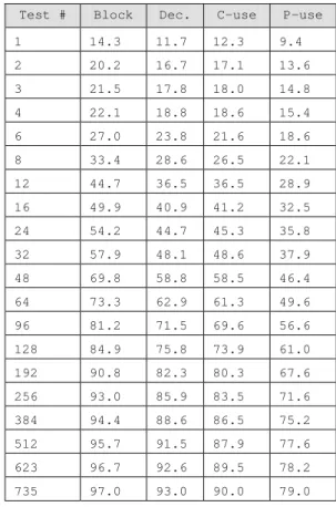
Table 4: analyze.c: Average coverage growth over 10 runs
Test # Block Dec. C-use P-use
1 14.3 11.7 12.3 9.4
2 20.2 16.7 17.1 13.6
3 21.5 17.8 18.0 14.8
4 22.1 18.8 18.6 15.4
6 27.0 23.8 21.6 18.6
8 33.4 28.6 26.5 22.1
12 44.7 36.5 36.5 28.9 16 49.9 40.9 41.2 32.5 24 54.2 44.7 45.3 35.8 32 57.9 48.1 48.6 37.9 48 69.8 58.8 58.5 46.4 64 73.3 62.9 61.3 49.6 96 81.2 71.5 69.6 56.6 128 84.9 75.8 73.9 61.0 192 90.8 82.3 80.3 67.6 256 93.0 85.9 83.5 71.6 384 94.4 88.6 86.5 75.2 512 95.7 91.5 87.9 77.6 623 96.7 92.6 89.5 78.2 735 97.0 93.0 90.0 79.0 Table 3: analyze.c: Coverage growth for a single run
Test # Block Dec. C-use P-use
1 23 16 23 18
2 42 32 39 32
3 42 32 39 32
4 42 32 39 32
6 50 40 43 36
8 50 40 43 36
12 50 40 43 36
16 50 40 44 37
24 64 45 60 41
32 75 59 65 48
48 81 69 69 55
64 81 70 72 58
96 81 72 73 59
128 88 79 78 64
192 94 87 83 72
256 94 87 83 73
384 94 89 85 75
512 94 90 86 77
623 96 92 89 78
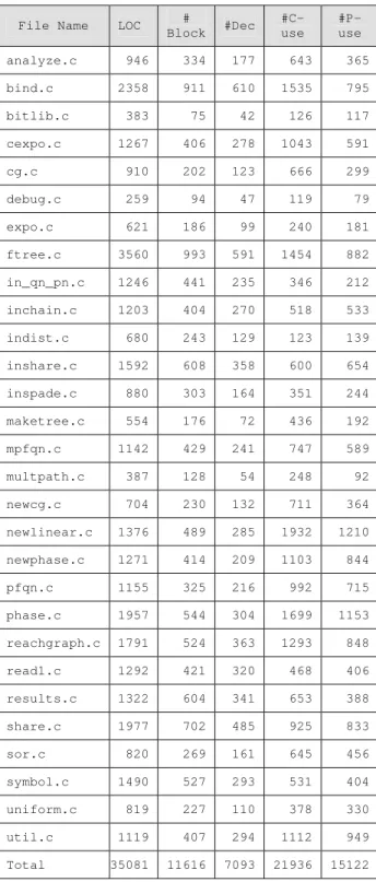
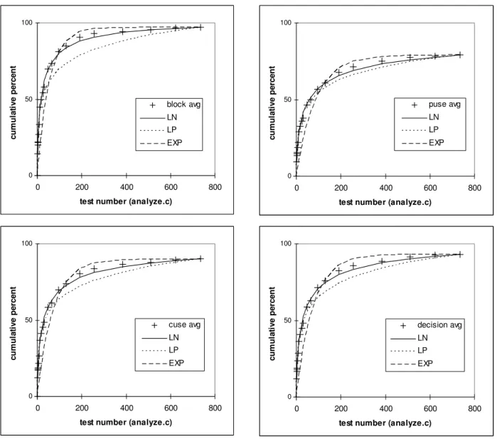
Figure 1: Cumulative coverage for analyze.c for four coverage measures.end_caption
Block: A basic block or simply a block is a sequence of instructions, which except for the last instruction is free of branches and function calls. A block may contain more than one statement if no branching occurs between the statements, a statement may contain multiple blocks if branching occurs inside the statement, an expression may contain multiple blocks if branching is implied within the expression. Also, in a basic block only the first statement can be a target of a branch.
Branch or Decision: A branch or a decision consists of a Boolean expression in its control structure.
C-use: A c-use is defined as a path through a program from each point where the value of a variable is defined to its computation use, without the variable being modified along the path.
P-use: A p-use is a path from each point where the value of a variable is defined to its use in a predicate or a
decision, without modifications to the variable along the path.
The execution time of each test case is assumed to be one. Thus the cumulative execution time is measured as the number of test cases executed. The level of coverage achieved for each measure for each file is in Table 2.
3.4. DATA REDUCTION AND AGGREGATION
ATAC reports block (decision, c-use, p-use) coverage in the form of percentage of blocks (decisions, c-uses, p-uses) executed. When the percentage coverage is reported, consecutive blocks (decisions, c-uses, p-uses) are treated to be independent. However, it may be the case that the consecutive blocks (decisions, c-uses, p-uses) are actually dependent.
It would be better for statistical analysis, to know the number of such independent sets or groups for each
0 50 100
0 200 400 600 800
test number (analyze.c)
cu
m
u
la
ti
ve p
e
rcen
t
block avg LN LP EXP
0 50 100
0 200 400 600 800
test number (analyze.c)
cu
m
u
la
ti
ve p
e
rcen
t
puse avg LN LP EXP
0 50 100
0 200 400 600 800
test number (analyze.c)
cu
m
u
la
ti
ve p
e
rc
en
t
decision avg LN LP EXP
0 50 100
0 200 400 600 800
test number (analyze.c)
cu
m
u
la
ti
ve p
e
rc
en
t
measure rather than the percentages. In any case, use of percentages (rather than the elements) will vary the absolute log-likelihood, but does not change the maximum likelihood estimates of the key lognormal parameters µ and σ. Likelihood ratio tests, log-likelihood differences, and AIC-computations are also unchanged by using percentages instead of counts provided the counts are on the order of 100. Standard deviations of the parameters were determined by inverting the Fischer Information Matrix [38].
We observed from the coverage data, that for each measure, some test cases are redundant and generate no additional coverage beyond the previous ones. A minimized test set which achieves the same level of coverage as the original one can thus be obtained for each measure [19] [34] [40]. For example, for block coverage less than 300 test cases achieve the same coverage as the entire suite of 735 test cases. Due to the presence of redundant test cases, we analyze the data by
dividing the whole execution sequence into 20 segments of proportionately increasing length. This makes it more likely that later buckets have at least some increase in the marginal coverage.
Cumulative coverage for each measure was obtained for each file of SHARPE and for the entire source code, for each run. As an example, for all measures we show the cumulative coverage for a single run, as well as the average over ten runs for the file analyze.c in Tables 3 and 4 respectively. It was observed that the cumulative coverage for individual files for a single run had very few increments, making it difficult to see true form of coverage growth. Therefore, for a single file, average cumulative coverage was computed using the cumulative coverage over ten runs to discover the mean function of coverage growth. This average cumulative coverage was used for analysis. Ten replications were chosen since it was visually observed that the average cumulative coverage computed using the data collected Table 5: SHARPE: Coverage growth for a single run
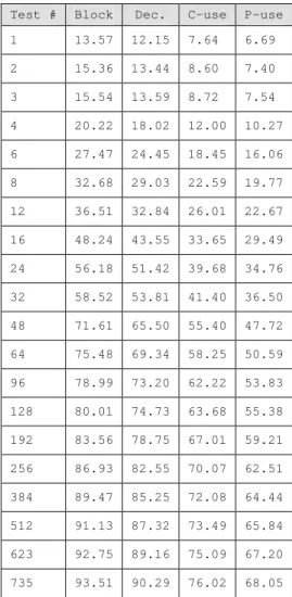
Test # Block Dec. C-use P-use 1 13.57 12.15 7.64 6.69 2 15.36 13.44 8.60 7.40 3 15.54 13.59 8.72 7.54 4 20.22 18.02 12.00 10.27 6 27.47 24.45 18.45 16.06 8 32.68 29.03 22.59 19.77 12 36.51 32.84 26.01 22.67 16 48.24 43.55 33.65 29.49 24 56.18 51.42 39.68 34.76 32 58.52 53.81 41.40 36.50 48 71.61 65.50 55.40 47.72 64 75.48 69.34 58.25 50.59 96 78.99 73.20 62.22 53.83 128 80.01 74.73 63.68 55.38 192 83.56 78.75 67.01 59.21 256 86.93 82.55 70.07 62.51 384 89.47 85.25 72.08 64.44 512 91.13 87.32 73.49 65.84 623 92.75 89.16 75.09 67.20 735 93.51 90.29 76.02 68.05
Table 6: SHARPE: Average coverage growth over 10 runs
over ten runs is reasonably smooth.
The coverage growth for the four measures for the entire SHARPE for a single run and average over ten runs is shown in Tables 5 and 6 respectively. Similar to Tables 3 and 4, Tables 5 and 6 also show the data divided into twenty segments. For the entire code coverage growth for a single run is also reasonably smooth. For the entire code, analysis was thus conducted using the coverage growth obtained from a single run and the average over ten runs.
4. ANALYSIS AND DISCUSSION
The data analysis is conducted in three parts, as follows: (a) Coverage growth for each measure for a single run and average over ten runs for a single file, namely, analyze.c, (b) Coverage growth for each measure for a single run and average over ten runs for the entire SHARPE application, (c) Comparative analysis of the coverage growth for each measure for average of ten sequences for individual files.
We will consider data sufficiency, run-to-run variation and the quality of the fits using log-likelihood (LLH), AIC and charts. We consider two alternative models, namely, the exponential model and the log-Poisson model. For the exponential model [M75], all blocks have identical execution rates, therefore the LLH
is the same as the lognormal with σ=0.0. For the log-Poisson (LP) model, we used the function [20].
)) ln( 1 ( )
(t a bt
M = +
to determine the MLE estimates of the parameters a and b
and use the associated LLH value.
The Akaike Information Criteria (AIC) can be computed for each model as follows [35]:
ters num_parame *
2 hood log_likeli
AIC=−2* +
The AIC is similar to a likelihood ratio test. It penalizes the model with more parameters, in this case the lognormal. The model with a lower AIC value is better. Two units of AIC is significant, four very significant [2].
4.1. ANALYSIS OF ANALYZE.C
The coverage growth of a single sequence and average over ten sequences for the file analyze.c are reported in Tables 3 and 4 respectively. An examination of the data in these tables provides some indication of how a particular replication differs from the overall average. To determine the average of all ten replications, we sum the coverage of each run;
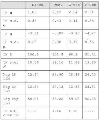
Table 8: analyze.c: comparative fits for average coverage growth
Block Dec. C-use P-use LN σ 1.83 2.12 2.14 2.34 LN s.d.
σ
0.34 0.43 0.44 0.56
LN µ -3.31 -3.87 -3.80 -4.27 LN s.d.
µ
0.26 0.38 0.39 0.56
LN N 100.6 101.8 98.2 91.42 LN s.d.
N
10.56 12.16 11.86 13.80
Neg LN LLH
25.94 23.90 28.93 26.55
Neg LP LLH
32.54 27.13 32.32 28.51
Neg Exp LLH
58.01 53.28 59.02 50.08
LN AIC over LP
11.2 4.46 4.78 1.92 Table 7: analyze.c: comparative fits for a single run
Block Dec. C-use P-use
LN σ 2.45 2.62 3.18 3.57 LN s.d.
σ
0.41 0.50 0.66 0.91
LN µ -2.51 -3.41 -3.02 -3.85 LN s.d.
µ
0.34 0.46 0.59 0.98
LN N 101.3 102.8 101.3 97.57 LN s.d.
N
10.72 12.47 13.25 18.18
neg LN LLH
77.41 68.36 60.38 51.12
neg LP LLH
78.53 69.78 61.07 51.00
neg Exp LLH
149.41 122.49 143.83 111.68
LN AIC over LP
determine the averages and the MLE fits of the models. The parameters of the LN are provided in Tables 7 and 8. Figure 1 shows the average coverage and the three MLE fits for block, decision, c-use and p-use coverage for the file analyze.c. It is shown in a linear form to illustrate the ability of the lognormal to fit both early and late data. Visually the lognormal is a better fit.
To form an objective judgment, we examined the log-likelihood of the data being generated by the three models. The LLH values reported in Tables 7 and 8 (for a single sequence and average over ten sequences respectively) indicate that the exponential model has far less likelihood of generating the observed data, than either the lognormal or the log-Poisson. Hence we will not analyze the exponential model any further.
Next we compare the log-Poisson and lognormal models using the AIC. The AIC values of analyze.c reported in Tables 7 and 8 (for a single sequence and average over ten sequences respectively) indicate that the lognormal can give the best fit for a single file, at least in this case when averaged over ten sequences. The parameters fitted to a single run, especially σ, can vary widely from the average; indeed the AIC for the selected
single run chose LP as a significantly better fit to the p-use data. The average growth is more likely to be generated by the lognormal than the log-Poisson for each coverage measure, and very significantly so for three.
4.2. ANALYSIS OF ENTIRE APPLICATION
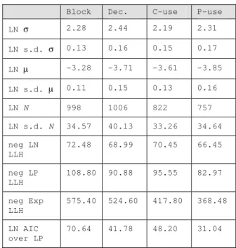
Because there is more activity (more increments) when summing coverage over the entire application, even coverage growth obtained from a single run provide sufficient data to constitute significant evidence. The LLH values for single runs in Table 9 show that the exponential model is a much poorer fit. The LLH are closer for LN and LP, so we use the AIC for comparison. For each measure the coverage growth is significantly better modeled by the lognormal even for the single sequence case.
To combine the ten replications of the whole, we formed and fitted their total in Table 10. With ten times the data, the uncertainty of is reduced to 0.17 or less. We find all four coverage measures have values of that are within 0.17 of 2.30. The similarity of the marginal coverage growth curves in Figure 2 reflects the closeness of values.
Table 9: SHARPE: comparative fits for a single run
Block Dec. C-use P-use LN σ 1.80 1.90 1.57 1.63
LN s.d. σ 0.34 0.37 0.34 0.38 LN µ -3.35 -3.60 -3.66 -3.77
LN s.d. µ 0.27 0.30 0.27 0.30 LN N 96.99 95.37 78.67 71.1 LN s.d. N 10.37 10.68 9.30 9.02 neg LN
LLH
46.91 44.91 42.27 39.30
neg LP LLH
53.06 49.08 47.12 42.89
neg Exp LLH
86.89 83.11 67.01 60.58
LN AIC over LP
10.3 6.34 7.7 5.18
Table 10: SHARPE: comparative fits for average coverage growth
Block Dec. C-use P-use LN σ 2.28 2.44 2.19 2.31
LN s.d. σ 0.13 0.16 0.15 0.17 LN µ -3.28 -3.71 -3.61 -3.85
LN s.d. µ 0.11 0.15 0.13 0.16
LN N 998 1006 822 757
LN s.d. N 34.57 40.13 33.26 34.64 neg LN
LLH
72.48 68.99 70.45 66.45
neg LP LLH
108.80 90.88 95.55 82.97
neg Exp LLH
575.40 524.60 417.80 368.48
LN AIC over LP
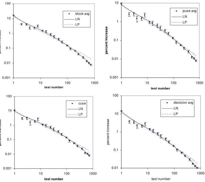
Figure 2: Marginal coverages as a function of number of tests
The advantage of the lognormal is most visible in Figure 2 which shows marginal (i.e. incremental) coverage per test for the four measures on a log-log scale. The fitted lines were generated from the parameters in Table 10. Ten replications were used to determine the standard deviation of the sample mean at each of the 20 points. For each coverage measure the data falls within one standard deviation of the lognormal fit over half the time, as expected.
4.3. ANALYSIS OF INDIVIDUAL FILES
As noted, in individual files there were considerably fewer increments (from 3 to 15) than for the entire application. This implies that there were intervals where no test caused any execution within a specific file. We
saw the consequences in case of analyze.c in Table 3. analyze.c was not atypical, but its coverage growth appeared somewhat less erratic than most files. Overall it is not useful to study coverage growth in single files, unless we replicate test realizations. Thus to discover the mean function for other files, we combine ten test realizations, as we did in analyze.c.
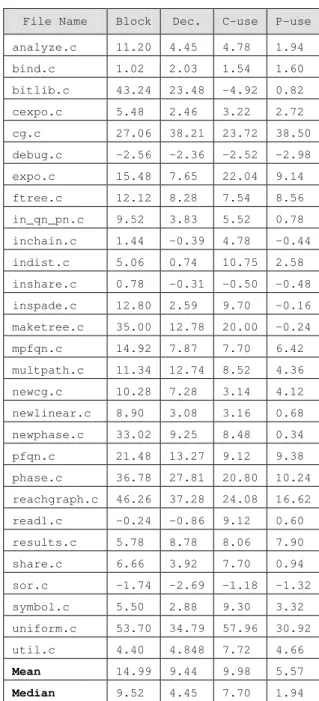
Table 11 provides the AIC advantage to the LN for each file for each coverage measure. For block, decision and c-uses, one or two are significantly more likely to be generated by the LP and 23 or more by the LN. Three or four others are inconclusive. For p-uses, although only debug.c seemed to fit the LP better, there were 12 that were equally likely to derive from the LP as the LN. As with SHARPE taken as a whole, we find the AIC
0.001 0.01 0.1 1 10 100
1 10 100 1000
test num ber
p
e
rcen
t in
cr
ease
block avg LN LP
0.001 0.01 0.1 1 10
1 10 100 1000
test number
p
e
rcen
t i
n
crease
puse avg LN LP
0.001 0.01 0.1 1 10 100
1 10 100 1000
test number
p
e
rcen
t i
n
crease
cuse LN LP
0.01 0.1 1 10 100
1 10 100 1000
test number
per
c
ent
inc
reas
e
decision avg LN
advantage to the LN is largest for block coverage, then less for c-use, decision, and p-use in that order. The same ranking applies if we consider either the mean or median of the AIC advantage over all 29 files.
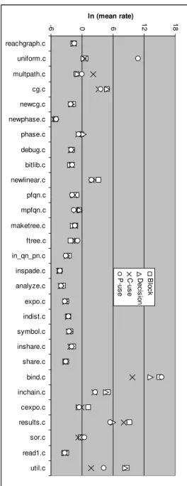
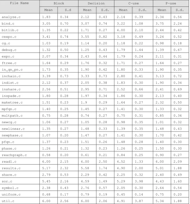
Tables 12 and 13 summarize the mean and the standard deviation of and for each file for each measure. The relative similarity of the four values is displayed in Figure 3, in which the files are ordered by of block coverage. We see the spread widening as exceeds 2.0, and becoming very erratic above 4.0. The mean value of a LN distribution can be computed as exp( +2/2). This must approximate the initial values of the total rate. Because the coverage measures initially grow at similar rates, we expect that these also will be very similar among the measures. We compare those in Figure 4. Again we find similarity among the values, but the greatest divergence is found among the files with large values of .
Bishop and Bloomfield [3] observed and explained a rough relationship between program size and the lognormal . The depth of conditionals is proportional to the log of the program size, and , the spread in the rates, is proportional to the square root of that. This relationship seems to imply that the elements of the different coverage measures exist at similar logical (or conditional depth) in the program. That is, the depth of a decision is nearly the same as the depth of the block it guards. Furthermore, the function will not vary much for files whose lengths barely range over a factor of ten. We found that the individual SHARPE files are the smallest studied to-date, and generally have values lower than those seen before, and lower than those of SHARPE as a whole. As seen already, some of the files were not convincingly fit by the lognormal and others yielded either high or erratic values of .
Figure 5 displays the relation between all four values and file size in LOC, for this application. Visually there is quite a bit of scatter, in particular due to the four files with > 4 and the largest file, which happens to have a low value. We find that for these 29 individual files there is only a weak dependence of on code size. The R-squared of a simple linear trend is less than .07 in every case. We interpret this as additional evidence that the conditions leading to the lognormal are not always present in single programs or small files. On the other hand, the behavior of SHAPE as a whole and many of its files are certainly fit by the lognormal. The depth of conditionals in files with fewer than 2000 LOC
are evidently too shallow to consistently approximate the conditions of the Central Limit Theorem and therefore may not always exhibit the lognormal. Above that size, and certainly with replication, the lognormal is generally observed
Table: 11: SHARPE files: Comparative AIC advantage
File Name Block Dec. C-use P-use analyze.c 11.20 4.45 4.78 1.94 bind.c 1.02 2.03 1.54 1.60 bitlib.c 43.24 23.48 -4.92 0.82 cexpo.c 5.48 2.46 3.22 2.72 cg.c 27.06 38.21 23.72 38.50 debug.c -2.56 -2.36 -2.52 -2.98 expo.c 15.48 7.65 22.04 9.14 ftree.c 12.12 8.28 7.54 8.56 in_qn_pn.c 9.52 3.83 5.52 0.78 inchain.c 1.44 -0.39 4.78 -0.44 indist.c 5.06 0.74 10.75 2.58 inshare.c 0.78 -0.31 -0.50 -0.48 inspade.c 12.80 2.59 9.70 -0.16 maketree.c 35.00 12.78 20.00 -0.24 mpfqn.c 14.92 7.87 7.70 6.42 multpath.c 11.34 12.74 8.52 4.36 newcg.c 10.28 7.28 3.14 4.12 newlinear.c 8.90 3.08 3.16 0.68 newphase.c 33.02 9.25 8.48 0.34 pfqn.c 21.48 13.27 9.12 9.38 phase.c 36.78 27.81 20.80 10.24 reachgraph.c 46.26 37.28 24.08 16.62 read1.c -0.24 -0.86 9.12 0.60 results.c 5.78 8.78 8.06 7.90 share.c 6.66 3.92 7.70 0.94 sor.c -1.74 -2.69 -1.18 -1.32 symbol.c 5.50 2.88 9.30 3.32 uniform.c 53.70 34.79 57.96 30.92 util.c 4.40 4.848 7.72 4.66
Mean 14.99 9.44 9.98 5.57
The Marginal Value of Increased Testing
An Empirical Anaysis
25
Figure 3:
of coverage measures for each file of SHARPE
Figure 4: Computed mean rates for each file of SHARPE
0 1 2 3 4 5 6
0
5
00
1000
1500
2000
2500
3000
3500
Lognormal sigma
Bl
o
c
k
D
e
ci
si
o
n
C-Us
e
P-U
s
e
-6 0 6 12 18
reachgraph.c
uniform.c
multpath.c
cg.c
newcg.c
newphase.c
phase.c
debug.c
bitlib.c
newlinear.c
pfqn.c
mpfqn.c
maketree.c
ftree.c
in_qn_pn.c
inspade.c
analyze.c
expo.c
indist.c
symbol.c
inshare.c
share.c
bind.c
inchain.c
cexpo.c
results.c
sor.c
ln (mean rate)
Bl
o
c
k
De
c
is
io
n
C-u
s
e
P-u
s
e
0 1 2 3 4 5 6
analyze.c
bind.c
bitlib.c
cexpo.c
cg.c
debug.c
expo.c
ftree.c
in_qn_pn.c
inchain.c
indist.c
inshare.c
inspade.c
maketree.c
mpfqn.c
multpath.c
newcg.c
newlinear.c
newphase.c
pfqn.c
phase.c
reachgraph.c
read1.c
results.c
share.c
sor.c
symbol.c
Lognormal sigma
Bl
o
c
k
De
c
is
io
n
C-u
s
e
P-u
s
Figure 5: Lognormal as a function of lines of code
4.4. IMPLICATIONS FOR TESTING
One of our objectives was to provide a quantitative feel for the similarities and differences among the growth characteristics of coverage measures. For this application, the number of code elements (blocks,
decisions, etc) differed by approximately a factor of three, with the most being p-uses and the least being decisions. The test suite used provided coverage exceeding 90% for blocks and decisions, but only close to three-quarters or two-thirds coverage for c-use and p-use respectively. It is unclear whether the lower c-p-use Table 12: SHARPE files: LN σ
Block Decision C-use P-use
File Name
Mean S.d Mean S.d. Mean S.d. Mean S.d. analyze.c 1.83 0.34 2.12 0.43 2.14 0.39 2.34 0.56
bind.c 3.05 0.70 3.07 0.74 3.22 1.08 3.75 2.24
bitlib.c 1.35 0.22 1.71 0.27 4.00 2.10 2.44 0.42
cexpo.c 3.41 0.74 3.55 0.82 3.18 0.49 3.24 0.52
cg.c 1.03 0.19 1.14 0.20 1.18 0.22 0.98 0.18
debug.c 1.32 0.50 1.25 0.43 1.79 1.44 1.39 0.67
expo.c 2.07 0.34 2.43 0.44 1.79 0.24 2.11 0.31
ftree.c 1.64 0.29 1.76 0.32 1.71 0.27 1.64 0.27
in_qn_pn.c 1.73 0.35 1.90 0.42 1.80 0.33 1.90 0.35 inchain.c 3.39 0.73 3.33 0.73 2.80 0.41 3.13 0.72
indist.c 2.12 0.37 2.05 0.38 1.83 0.30 1.90 0.34
inshare.c 2.56 0.51 2.95 0.71 2.52 0.66 2.41 0.69 inspade.c 1.80 0.28 1.97 0.34 1.86 0.30 2.13 0.40 maketree.c 1.51 0.23 1.9 0.29 1.64 0.27 2.32 0.50
mpfqn.c 1.40 0.25 1.45 0.27 1.41 0.30 1.33 0.32
multpath.c 0.75 0.28 0.74 0.27 0.75 0.31 0.85 0.36
newcg.c 1.06 0.27 1.05 0.28 0.98 0.35 1.01 0.32
newlinear.c 1.35 0.27 1.48 0.33 1.39 0.35 1.48 0.43 newphase.c 1.07 0.20 1.47 0.27 1.41 0.30 1.70 0.42
pfqn.c 1.37 0.23 1.51 0.26 1.48 0.28 1.40 0.30
phase.c 1.26 0.21 1.32 0.23 1.26 0.25 1.50 0.30
reachgraph.c 0.58 0.20 0.61 0.21 0.84 0.25 0.90 0.27
read1.c 6.00 2.15 6.00 2.50 4.52 1.33 6.00 2.09
results.c 5.17 2.32 5.58 1.74 4.90 2.00 5.01 1.88
share.c 2.79 0.53 2.29 0.42 2.25 0.32 2.40 0.49
sor.c 5.45 2.16 4.59 1.49 5.29 3.98 4.43 1.60
symbol.c 2.38 0.43 2.76 0.57 2.05 0.30 2.64 0.54
uniform.c 0.68 0.17 0.79 0.19 0.45 0.14 0.75 0.20
and p-use coverage is due to their being “more numerous, demanding, and thorough” or merely “including infeasible cases”.
With few exceptions these orderings, if not the exact ratios, held for the individual files as well. Because the growth curves follow from lognormal behavior seen in other applications, as well as in files within this application, we believe our results are of general interest.
Our results confirming lognormal coverage growth together with the proportionality proposed by Bishop and Bloomfield [3] allow us to establish an important connection between a dynamic phenomenon which is manifested through code execution (namely, code coverage growth) and the static structure of the code. This connection can be exploited to estimate of the lognormal coverage growth model by examining static aspects of the code such as its size or logical depth. Further, the parameter of the lognormal, which is a Table 13: SHARPE files: LN µ
Block Decision C-use P-use
File Name
Mean S.d. Mean S.d. Mean S.d. Mean S.d. analyze.c -3.31 0.26 -3.87 0.38 -3.80 0.39 -4.27 0.56 bind.c -4.07 0.74 -4.43 0.23 -4.71 1.08 -3.75 2.24 bitlib.c -2.08 0.19 -2.32 0.54 -5.80 2.10 -3.05 0.42 cexpo.c -1.02 0.48 -1.48 0.19 -1.82 0.49 -1.69 0.52
cg.c -2.33 0.18 -2.58 0.85 -2.82 0.22 -2.74 0.18
debug.c -6.02 0.66 -5.78 0.52 -7.03 1.44 -6.00 0.67 expo.c -2.38 0.27 -2.66 0.34 -2.32 0.24 -2.91 0.30 ftree.c -3.34 0.24 -3.50 0.27 -3.65 0.27 -3.52 0.27 in_qn_pn.c -3.52 0.27 -4.08 0.36 -3.62 0.33 -3.76 0.35 inchain.c -2.62 0.60 -3.37 0.70 -2.05 0.41 -3.12 0.72 indist.c -3.35 0.32 -3.87 0.36 -3.09 0.25 -3.76 0.30 inshare.c -3.89 0.51 -4.76 0.89 -4.27 0.70 -4.54 0.76 inspade.c -2.92 0.24 -3.67 0.31 -3.04 0.26 -3.73 0.38 maketree.c -3.40 0.20 -2.72 0.25 -2.68 0.23 -3.62 0.47 mpfqn.c -3.52 0.20 -3.95 0.23 -3.94 0.24 -4.05 0.25 multpath.c -4.62 0.16 -4.56 0.16 -4.74 0.17 -4.73 0.22 newcg.c -4.26 0.19 -4.50 0.21 -4.64 0.26 -4.65 0.24 newlinear.c -4.00 0.22 -4.32 0.28 -4.20 0.29 -4.50 0.37 newphase.c -3.24 0.17 -3.74 0.23 -3.68 0.25 -4.13 0.38 pfqn.c -3.20 0.19 -3.41 0.22 -3.64 0.24 -3.60 0.25 phase.c -2.56 0.19 -2.81 0.20 -3.03 0.21 -3.24 0.26 reachgraph.c -3.24 0.15 -3.44 0.16 -3.54 0.18 -3.59 0.20 read1.c -3.08 2.17 -4.81 3.03 -0.47 0.68 -2.72 1.98 results.c -8.45 5.16 -10.93 4.83 -9.58 5.00 -10.04 4.94 share.c -2.79 0.39 -3.22 0.36 -2.61 0.32 -3.47 0.45
sor.c -5.75 3.40 -4.52 1.91 -5.92 3.98 -4.46 2.00
location parameter in the corresponding reliability growth model, is here a measure of individual test efficiency. As such an approximate estimate of may be obtained from previous projects by the same team. Finally, in a reliability growth model a third parameter, N, represents the ultimate number of defects and must be estimated – in fact this is the key purpose of such a model.
Since there is no a priori limit on the number of defects, the error in the estimated value of N may be quite large. But in the case of code coverage the total number of code elements provides a known upper bound. As indicated in Section 2.3, in the coverage growth model, the estimated value of N will represent the coverage that can be feasibly achieved, given infinite testing time and resources. This estimated value of N may fall short of the upper bound by the number of unreachable elements, i.e. those that cannot be executed.
Referring to Table 6 and Figure 2 it can be observed that the coverage for all the four measures was increasing with additional testing, right up to the last test interval. Although the coverage values at the end of the last interval represent what can be achieved with our given test suite, this implies that additional tests are likely to increase the coverage further, to a point where all the feasible code is covered. The estimates of N obtained through fitting the lognormal model can then provide a projection of the level of feasible coverage. The values of N in Table 10 estimate approximately 100% feasible coverage for both block and decision coverage measures. The other two measures, however, are converging on lower values, namely, 78.67% for p-use coverage and 82.8% for c-p-use coverage. It is important to note that the model does not assume that achieving 100% coverage is feasible. The fit is based on the shape of the growth curve, not on an expectation that it will reach 100%..
A significant outcome of these results is that approximate estimates of the parameters describing coverage growth can be obtained a priori, even before testing commences. This advance knowledge can be used to control the testing process or to decide a specific testing strategy by enabling projections regarding the amount of testing necessary to achieve a certain level of coverage. For example, if over 50% of the coverage can be gained by executing only a randomized 10% of the test cases, it suggests the strategy of initially testing a new product by rapidly interleaving truncated test cycles with periods of defect reproduction, debug, and fix.
The parameter estimates obtained a priori can also be used to estimate the marginal effort needed to achieve a certain improvement in coverage. Such
marginal effort is a function of of the lognormal because the shape of the growth curve depends on this parameter. For the sake of illustration, the relative testing effort necessary to improve coverage from 75% to 90% (95% and 99%) for different values of is tabulated in Table 14. In each row the effort to achieve 75% coverage has been normalized to unity in order to remove dependencies on other characteristics. Referring to the table, it can be observed that for = 0 the number of tests necessary to cover 99% of the code is double the number required to cover 90%.. A zero value of corresponds to a “memoryless” exponential decay process, which is the easiest case, but an uncommon one. For realistic values of , the proportion of additional tests needed for this additional percentage coverage is a sensitive function of and increases rapidly. Finally, since the value of is proportional to a function of the size or the logical depth of the program [3], practical coverage goals can be established in advance, independent of problem domain.
5. CONCLUSIONS AND FUTURE RESEARCH
In this paper we study the growth characteristics of four coverage measures, namely, block, decision, c-use and p-use. We hypothesize and empirically establish that the coverage growth for each one of the coverage types can be derived from a lognormal distribution. In addition, we also confirm the hypothesis that the parameters of the lognormal distribution for each one of the coverage types are close. By using randomized repetitive test sequences we empirically and quantitatively unify concepts from software test sufficiency, test efficiency and reliability growth. We then discuss how the lognormal coverage growth model could be used to guide and control the testing process by providing estimates of marginal testing effort to achieve different degrees of coverage improvements.There are several related questions that provide opportunities for further research. What would be the impact of generating test suites by randomly sampling
Table 14: Relative testing needed to increase coverage from75% to 90%, 95%, and 99% as a function of LN
LN σ 75% 90% 95% 99%
0 1 1.67 2.18 3.36
1 1 2.30 3.71 8.87
2 1 3.94 8.84 39.7
3 1 6.96 22.10 190.8
test suites with replacement, instead of without replacement as used in this paper? Directly measuring the execution of the code elements (as was done by [3]), determining whether that distribution is lognormal as expected, and then comparing those parameters to the ones obtained from code coverage growth data would provide a useful cross-check. The three-way relationship between code coverage growth, test-count, and test execution time needs to be established. A related opportunity is the further exploration of how the size of programs (measured in various ways) affects the parameters of the lognormal for each coverage measure. Given that, it should be possible to do predictions based on a combination of early test experience with prior static information bounding lognormal , , and the number of code elements.
The techniques used in this paper, particularly that of measuring coverage achieved by randomized sequences of tests, could well be used to determine the practical limits on the accuracy of coverage and defect predictions.
ACKNOWLEDGMENTS
We thank Dr. Bob Horgan of Telcordia Technologies for giving us access to ATAC. We thank Prof. Kishor Trivedi of Duke University for the source code of SHARPE, and Dr. Robin Sahner for the SHARPE test suite. We thank Cisco management, especially Tricia Baker and John Intintolo, for their encouragement. The research at Univ. of Connecticut was supported in part by a Large Grant from the Univ. of Connecticut Research Foundation and in part by a CAREER award (#CNS-0643971) from the National Science Foundation.
REFERENCES
[1] J. Aitchison and J.A.C. Brown, The Lognormal Distribution, Cambridge University Press, NY, 1969.
[2] H. Akaike, Prediction and Entropy, MRC Technical Summary Report #2397, NTIS, Springfield, VA, 1982.
[3] P. Bishop and R. Bloomfield, Using a Log-normal Failure Rate Distribution for Worst Case Bound Reliability Prediction. In Proceedings of International. Symposium on Software Reliability Engineering, pages 237-245, 2003.
[4] L. Briand and D. Pfahl, Using simulation for assessing the real impact of test coverage on defect coverage, IEEE Transactions on Reliability, 49(1): 60-70, 2000.
[5] M. H. Chen, M. R. Lyu and W. E. Wong, Effect of code coverage on software reliability measurement, IEEE Transactions on Reliability, 50(2): 165-170, 2001.
[6] L. Clarke, A. Podgurski, D. J. Richardson and S. J. Zeil, A formal evaluation of data flow path selection criteria, IEEE Transactions on Software Engineering, 15(11): 1318-1332, 1989.
[7] E.L. Crow and K. Shimizu, ed., Lognormal Distributions: Theory and Applications, Marcel Dekker, NY, 1988.
[8] S. R. Dalal, J. R. Horgan and J. R. Kettenring, Reliable software and communications: Software quality, reliability and safety. In Proceedings of International. Conference on Software Engineering, pages 425-435, 1993.
[9] E. Diaz, J. Tuya and R. Blanco, A modular tool for automated coverage in software testing. In Proceedings of Eleventh Annual International Workshop on Software Technology and Engineering Practice, pages 241-246, 2003.
[10] P. Frankl and P. J. Weiss, An experimental comparison of the effectiveness of branch testing and data flow testing, IEEE Transactions on Software Engineering, 19(8): 747-787, 1993.
[11] A. L. Goel and K. Okumoto, Time-dependent error detection rate models for software reliability and other performance measures, IEEE Transactions on Reliability, R-28(3): 206-211, 1979.
[12] S. Gokhale and R. Mullen, From test count to code coverage using the Lognormal. In Proceedings of International Symposium on Software Reliability Engineering, pages 295-395, 2004.
[13] S. Gokhale and K. S. Trivedi, A time/structure based software reliability model, Annals of Software Engineering, 8: 85-121, 1999.
[14] M. Grottke, A vector Markov model for structural coverage growth and number of failure occurrences. In Proceedings of International Symposium on Software Reliability Engineering, pages 304-315, 2002.
[15] H. Hirose, Estimation of threshold stress in accelerated life-testing, IEEE Transactions on Reliability, 42(4): 650-657, 1993.
[17] J.R. Horgan and S.A. London, Dataflow Coverage and the C Language. In Proceedings of Fourth International Symposium on Testing, Analysis and Verification, pages 87-97, 1991.
[18] .L. Johnson, S. Kotz, and N. Balakrishnan, Continuous Univariate Distributions, vol. 1, Wiley, New York, 1994.
[19] J. A. Jones and M. J. Harrold, Test-suite reduction and prioritization for modified condition/decision coverage, IEEE Transactions. on Software Engineering, 29(3): 195-209, 2003.
[20] P. A. Keiller and D. R. Miller, On the use and performance of software reliability growth models, Reliability Engineering and Systems Safety, 32: 95-117, 1991.
[21] M. R. Lyu, J. R. Horgan and S. London, A coverage analysis tool for the effectiveness of software testing, IEEE Transactions on Reliability, 43 (4): 527-535, 1994.
[22] Y. K. Malaiya, N. Li, J. Beiman and R. Karcich, Software reliability growth with test coverage, IEEE Transactions on Reliability, 51(4): 420-426, 2002.
[23] Y. Malaiya, N. Li, J. Beiman et al., The relationship between test coverage and reliability, In Proceedings of International Symposium on Software Reliability Engineering, pages 186-195, 1994.
[24] D.R. Miller, Exponential Order Statistic Models of Software Reliability Growth, NASA Contractor Report 3909, NTIS, Springfield, VA 22161, 1985.
[25] S. Misra, Evaluating four white-box test coverage methodologies. In Proceedings of IEEE Canadian Conference on Electrical and Computer Engineering, pages 1739-1743, 2003.
[26] R.E. Mullen, The Lognormal distribution of software failure rates: Application to software reliability growth modeling. In Proceedings of International Symposium on Software Reliability Engineering, pages 134-142, 1998.
[27] R.E. Mullen, The Lognormal distribution of software failure rates: Origin and evidence. In Proceedings of International Symposium on Software Reliability Engineering, pages 124-133, 1998.
[28] J. D. Musa, A theory of software reliability and its application, IEEE Transactions on Software Engineering, SE-1(1): 312-317, 1975.
[29] R. Mullen and S. Gokhale, Software defect rediscoveries: A Discrete Lognormal model. In
Proceedings of International Symposium on Software Reliability Engineering, pages 203-212, 2005.
[30] R. Mullen and S. Gokhale, A Discrete Lognormal model for software defects affecting QoP. In Quality of Protection: Security Measurements and Metrics, D. Gollmann and F. Massacci and A. Yautsiukhin (Eds.), pages 37-48, Advances in Information Security Series, Springer Verlag, 2006.
[31] W. Nelson, Accelerated Testing, Wiley, New York, 1990.
[32] P. Netisopakul, L. J. White, and J. Morris, Data coverage testing. In Proceedings of Asia Pacific Software Engineering Conference, pages 465-472, 2002.
[33] P. Piworaski, M. Ohba and J. Caruso, Coverage measurement experience during functional test. In Proceedings of International Conference on Software Engineering, pages 287-293, 1993.
[34] S. Rapps and E. J. Weyuker, Selecting test data using data flow information, IEEE Transasctions on Software Engineering, SE-11(4): 367-375, 1985.
[35] Y. Sakamoto, M. Ishiguro, and G. Kitagawa, Akaike Information Criterion Statistics, D.Reidel, Holland, 1986.
[36] R. A. Sahner, K. S. Trivedi and A. Puliafito, Performance and Reliability Analysis of Computer Systems: An Example-Based Approach Using the SHARPE Software Package, Kluwer Academic Publishers, Boston, 1996.
[37] S. K. S. Sze and M. R. Lyu, ATACOBOL – a COBOL test coverage analysis tool and its applications. In Proceedings of International Symposium on Software Reliability Engineering, pages 327-335, 2000.
[38] K. S. Trivedi, Probability and Statistics with Reliability, Queuing and Computer Science Applications, John Wiley and Sons, New York, 2001.
[39] M. Vouk, Using reliability models during testing with non operational profiles. In Proceedings of Second Bellcore/Purdue workshop on Issues in Software Reliability Estimation, pages 103-111, 1992.