MEASURES OF IRREGULARITY OF GRAPHS
Joelma Ananias de Oliveira
1, Carla Silva Oliveira
2,
Claudia Justel
3and Nair Maria Maia de Abreu
4*Received June 13, 2012 / Accepted March 15, 2013
ABSTRACT.A graph is regular if every vertex is of the same degree. Otherwise, it is an irregular graph. Although there is a vast literature devoted to regular graphs, only a few papers approach the irregular ones. We have found four distinct graph invariants used to measure the irregularity of a graph. All of them are determined through either the average or the variance of the vertex degrees. Among them there is the index of the graph, a spectral parameter, which is given as a function of the maximum eigenvalue of its adjacency matrix. In this paper, we survey these invariants with highlight to their respective properties, especially those relative to extremal graphs. Finally, we determine the maximum values of those measures and characterize their extremal graphs in some special classes.
Keywords: index of a graph, irregularity measure, extremal graphs.
1 INTRODUCTION
LetG be an undirected graph withn vertices andmedges without loops and multiple edges. We denoteG(n)andH(n), the respective sets of all the graphs (connected or not) and all the connected graphs withn vertices and,G(n,m)andH(n,m), the respective sets of the graphs (connected or not) and all the connected graphs withn vertices andm edges. Thedegreeof a vertexvi, denotedd(vi), is the number of the incident edges invi. Sincei=1,nvi =2m, the average of vertex degreescan be given asd(G)= 2nm. A graph isk-regular or, simply regular, if every degree is equal tok. Otherwise, the graph is said to be anirregular graph.
The eigenvalues of a graph are the eigenvalues of its adjacency matrix. They are also respectively referred as theA-eigenvalue, denotedλ1≥λ2≥. . .≥λn. The index of a graph is the maximal eigenvalue ofA(G), that is,λ1(G). The joinG1∨G2of (disjoint) graphsG1andG2is the graph obtained fromG1andG2by joining each vertex ofG1with each vertex ofG2.
*Corresponding author
1Universidade Federal de Mato Grosso, Brasil. E-mail: [email protected]
2Escola Nacional de Ciˆencias Estat´ısticas, Rio de Janeiro, Brasil. E-mail: [email protected] 3Instituto Militar de Engenharia, Rio de Janeiro, Brasil. E-mail: [email protected]
384
MEASURES OF IRREGULARITY OF GRAPHSGiven a graphG,what is the minimal number of edges needed to add to G to get H , a regular supergraph of G?In this case, which pairs of non adjacent vertices in G should become adjacent in H? Questions such as these are interesting and in order to try to answer them it seems useful to know how near or distant any graph is from a regular one. We define as themeasure of irregularity
ofG,every functionF : G → R, whereGis the set of all graphs andRis the set of all real number, such that∀G∈G,Gis a regular graph if and only ifF(G)=0.
In this paper, we survey all known parameters used as measures of irregularity as well as their respective properties, mainly those relative to upper and lower bounds and their respective ex-tremal graphs. Also, we characterize their exex-tremal graphs among all the split complete graphs and among all path complete graphs with a particular characteristic.
2 KNOWN MEASURES OF IRREGULARITY
In 1957, Collatz & Sinogowitz [8] proved that the index of a graph is greater than or equal to the average of vertex degrees and the equality holds if and only if the graph is regular. From this fact, they introducedε(G)=λ1(G)−d(G)to measure the irregularity of a graph, which we call here, thespectral measure. Those authors also proved that, forn≤5, the maximum value toε(G)is
√
n−1−2+2n and the maximal is attained for the starSn. Based on this, they conjectured that Snis the most irregular graph among all graphs withn vertices relative toε(G). In 1988, this conjecture was refuted by Cvectkovi´c & Rowlinson [9].
Some years after, Bell [4] suggested making the variance of the degrees of the vertices ofG,
σ (G)= 1 n
n
i=1
(d(vi))2− 1
n2
n
i=1
d(vi) 2
,
as a measure of the irregularity ofG, and we refer to it as thevariance measure. Bell charac-terized the most irregular graphs in the classesG(n),G(n,m)andH(n,m)concerning the both measuresε(G)andσ (G). In the same paper, he obtained upper and lower bounds ofσ (G)as functions ofnandm.
Albertson [2] defined the imbalance of an edge(vi, vj)byimbvivj = |d(vi)−d(vj)|and he used it to introduceirr(G) = (vi,vj)∈Eimbvivj as a measure of the irregularity ofG and, in the same paper, irr(G) < 427n3 is proven. In 2000, Hansenet al.[10] presented a bound to
irr(G) as a function ofn and m and determined extremal graphs for it. Here, we refer this invariant as theimbalance measure.
More recently, Nikiforov [13] introduceds(G) =vi∈V(G)d(vi)− 2nm
as a new measure of
the irregularity of a graph. Also, he showed several inequalities with respect tos(G),ε(G)and
σ (G). The measure of Nikiforov will be named by thedegree deviation measure.
It is easy to see thatε(G), σ (G)ands(G)can be taken byF(G), sinceε(G)=σ (G)=s(G)=
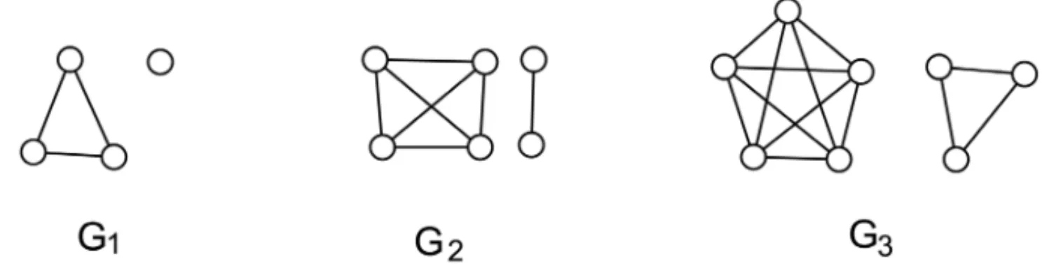
0 if and only if G is a regular graph. Although irr(G) is considered in the literature as an irregularity measure, it can be null even whenGis an irregular graph. In this case,irr(G)=0 if
and only ifGis either regular or a disconnected graph with all the regular components. Figure 1 illustrates this fact.
Figure 1– Disconnected graphs such thatirr(G1)=irr(G2)=irr(G3)=0.
3 EXTREMAL IRREGULARITY IN GENERAL CLASSES OF GRAPHS
This section is devoted to define the families of graphs where some elements are extremal for
ε(G),σ (G)andirr(G)whereGis a graph belonging to one of the most general classes such as G(n), H(n), G(n,m)andH(n,m). Then, theorems are presented to show the conditions under which those graphs are extremal for the measures studied. The section ends with a table summarizing these results.
Definition 3.1. [1] A graph with n vertices and m edges is a quasi-complete graph, denoted QC(n,m), when it is obtained as follows:
(i) its vertices are labeled1, . . . ,n;
(ii) the integers d and t ,2≤d,0≤t <d, are defined such that m=d2+t ;
(iii) the vertices labeled1, . . . ,d form the maximal clique;
(iv) the vertex d+1is adjacent to t vertices labeled1, . . . ,t and the n−(d +1)remaining vertices are isolated.
Figure 2 displays some examples of quasi-complete graphs.
386
MEASURES OF IRREGULARITY OF GRAPHSThe first result, due to Bell [4], gives the maximum value of the spectral measure, ε(G), where
Gis a graph (not necessarily connected) withnvertices. Moreover, it shows that the extremal graphs toε(G) are the quasi-complete graphs. Proposition 3.2, also due to Bell, proves that among all graphs withn vertices andm edges, no necessarily connected, the quasi-complete graphQC(n,m)is the only one that satisfies the maximal value of the spectral measure.
Proposition 3.1.[4] Given n, write m=⌊12(n+1)⌋ 2
and m′=⌊12(n+1)⌋+1 2
. Then, we have
max{ε(G):G∈G(n)} = ⎧ ⎪ ⎪ ⎨
⎪ ⎪ ⎩
1 4n−
1
2 (neven); 1
4n− 1 2+
1
4n (nodd).
This maximum is attained uniquely by QC(n,m)if n is odd, and by QC(n,m)and QC(n,m′) (only) if n is even.
For example, ifn =6, max{ε(G) : G ∈ G(6)} =1 and Gis eitherQC(6,3)= K3∪3K1or
QC(6,6)=K4∪2K1.
Proposition 3.2. [4] Let n and m be given with m ≤ n2. Then,max{ε(G) : G ∈ G(n,m)}is attained uniquely by QC(n,m).
The following result gives the maximum value of the variance measure,σ (G), whenGis a graph withnvertices, and it proves that the maximum is attained whereGis a quasi-complete graph.
Proposition 3.3. [4] Given n, write r = ⌊14(3n+2)⌋and m =r2. Then, we havemax{σ (G): G∈G(n)} = r
n2(r −1)2(n−r), and this maximum is attained by QC(n,m).
For example, ifn =7, max{σ (G):G∈G(7)} =3,26 andGisQC(7,10)=K5∪2K1. For specific values ofnandm, the quasi-star graphs, defined as follows, give the extremal graph to the variance measure in the class of the connected graphs withnvertices.
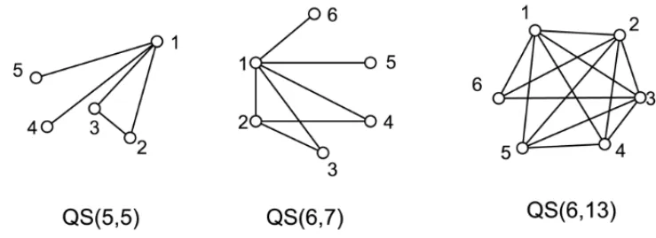
Definition 3.2.[1] A quasi-star, denoted Q S(n,m), is a graph with n vertices and m edges when it is obtained as follows:
(i) its vertices are labeled1, . . . ,n;
(ii) the integers d and t ,2≤d,0≤t <d, are defined such that m=n2−d2−t ;
(iii) the first n−d−1vertices are adjacent to all others vertices of the graph;
(iv) the vertex n−d is adjacent to vertices labeled1, . . . ,n−t .
The Figure 3 shows quasi-star graphs with 5 and 6 vertices.
The next result is an immediate consequence of Proposition 3.4 and it was presented in [4] as its corollary. Proposition 3.5 shows that among all graphs withnvertices andmedges, the extremal
Figure 3– GraphsQ S(5,5),Q S(6,7)andQ S(6,13).
ones relative to the variance measure are quasi-stars Q S(n,m), when they are sparse graphs; otherwise, the extremal graphs are quasi-completeQC(n,m).
Proposition 3.4. [4] Given n, write r = ⌊14(3n +2)⌋and m = n2−r2. Then, we have
max{σ (G):G∈H(n)} = r
n2(r −1) 2(n
−r), and this maximum is attained by Q S(n,m).
For example, ifn=7, max{σ (G):G∈H(7)} =3,26 andGisQ S(7,11)=K1∨K1,5.
Proposition 3.5.[4] Let n and m be given, with m ≤n2. Then, themax{σ (G):G∈G(n,m)} is attained by QC(n,m)if m> 12n2+n2, and by Q S(n,m)if m< 12n2−n2.
For example, ifn=6 andm=11, max{σ (G):G∈H(6,11)} =1,55 andGisQC(6,11)= K1∨(K4∪K1). Ifn=6 andm=4, max{σ (G):G∈H(6,4)} =1,55 andGisQ S(6,4)=
S5∪K1.
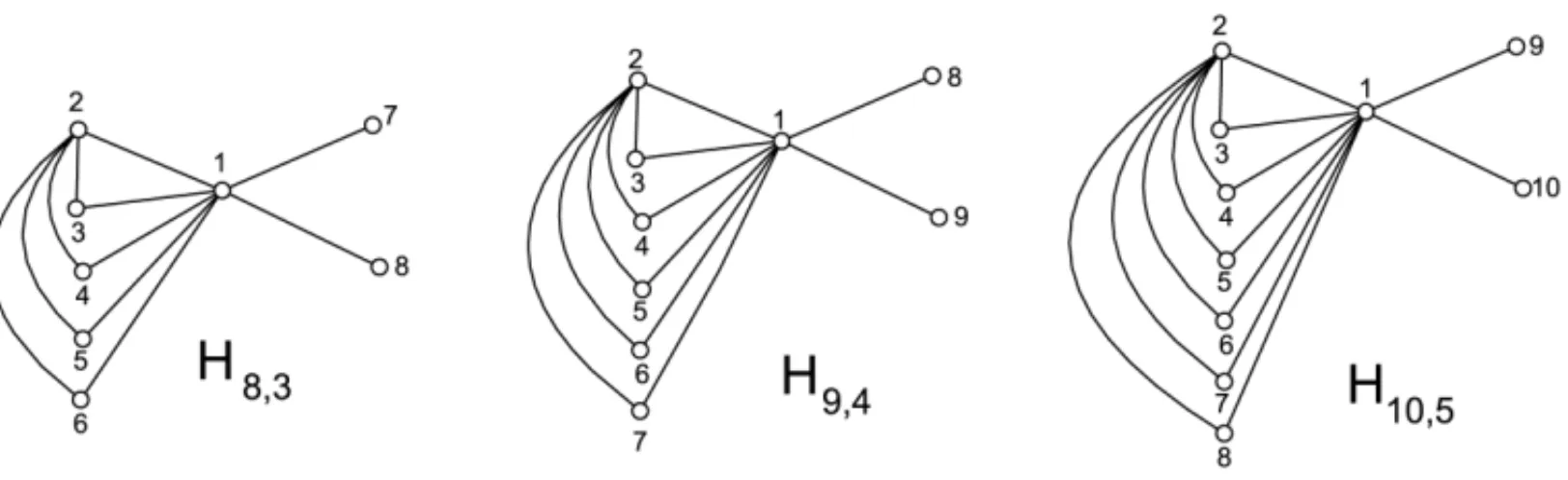
Definition 3.3.[7] Let0≤k≤n−3and let Hn,kbe a connected graph with n+k edges. Hn,k is obtained as follows:
(i) label the vertices from1to n;
(ii) add n−1edges from the vertex labeled1to2, . . . ,n (a star Snwith center in1); (iii) add k edges from the vertex 2 to each vertex3, . . . ,k+3.
The graphs Hn,k result from the following joinHn,k = K1∨(K1,k+1 ∪Kn−k−3). Similar to
them, Definition 3.4 introduces the graphsGn,k. For a large enoughn, the first graphs satisfy the maximum value to the spectral measure among all connected graphs withn vertices andn+k
edges; the second graphs satisfy the maximum values of the variance measure among all non sparse connected graphs withnvertices. Some examples of graphsHn,kare shown in Figure 4.
388
MEASURES OF IRREGULARITY OF GRAPHSFigure 4– GraphsH8,3,H9,4andH10,5.
Definition 3.4. [9] For k ∈ Zsuch that0 ≤ k < n(n2−3), Gn,k results of the join of K1and
QC(n−1,k), that is, Gn,k =K1∨QC(n−1,k). See some examples of graphsGn,k in the Figure 5.
Figure 5– GraphsG6,0,G7,1andG7,2.
Proposition 3.7.[4] If n and m=n+k are such that n−1≤m≤n2, thenmax{σ (G):G∈ H(n,m)}is attained by Gn,k if m>12
n 2
+n−1, and by Q S(n,m)if m< 12n2.
Definition 3.5.[3] Given n and q integers such that0≤q ≤n, a pineapple graph, denoted by P A(n,q), is a graph with n vertices consisting of a clique on q vertices and a stable set on the remaining n−q vertices in which each vertex of the stable set is adjacent to a unique and the same vertex of the clique.
Aouchicheet al., in [3], conjectured that, among all connected graphs withn vertices, the max-imal relative to the spectral measure are the pineapple graphs such that the size of the maxmax-imal clique is one or two unities more than the size of the maximal stable set.
Conjecture 3.1. [3] The most irregular graph toε(G), where G is a connected graph on n (n≥10)vertices, is a pineapple P A(n,q))in which the clique size q is equal to⌊n2⌋ +1.
Finally, it follows the definition of the family of graphs which are maximal to the imbalance measure.
Definition 3.6. [3] Given n,k and t integers such that t ≤ k ≤ n, a fanned complete split graph, denoted by FC S(n,k,t), is a graph with n vertices obtained from a complete split graph C S(n,k)by connecting a vertex from the stable set by edges to t other vertices of the stable set.
Theorem 3.1.[10] For any graph G with n vertices, m edges and irregularity irr(G), irr(G)≤k(n−k)(n−k−1)+t(t−2k−1)
where
k=
n−1
2 −
n−1
2
2
−2m
and
t =m−(n−k)k−k(k−1)/2.
Moreover, this value is attained if and only if G is a fanned complete split graph.
The Figure 6 shows the extremal fanned complete split graph with 8 vertices and 15 edges for imbalance measure, whereirr(FC S(8,2,2))=54.
Figure 6– GraphFC S(8,2,2).
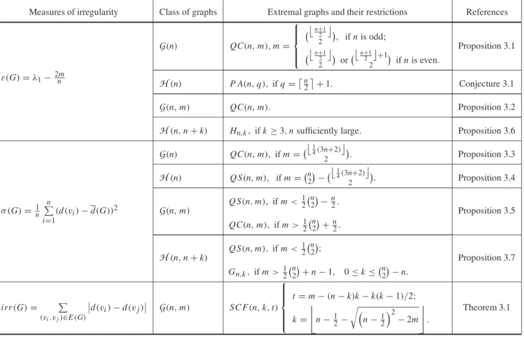
Table 1 shows, in each line of the third column, the extremal graph among all graphs in the class on the correspondent line of the second column. Each extremal graph is relative to the irregularity measure displayed in the same line of the first column. The last column gives the references that support those results.
4 EXTREMAL IRREGULARITY IN PCn,p,1ANDSC(n,k)GRAPHS
The results presented in this section come originally from [14] and approach the following connected graphs with ordern: the graphs PCn,p,1 =K1,n−p−1∪p K1, which are special case of path complete graphs (see Definition 4.1, [5], [12]) and the complete split graphsSC(n,k), special cases of the well known split graphs, (see Definition 4.2 and [6]).
Definition 4.1.Let n,m,p,t∈N, with1≤t ≤n−2and1≤ p≤n−t−1. A graph with n vertices and m edges such that
(n−t)(n−t−1)
2 +t≤m≤
(n−t)(n−t−1)
2 +n−2
390
M E A S URE S O F IRRE G U L A RIT Y O F G R A P H STable 1– Extremal graphs for measures of irregularityε(G), σ (G)andirr(G).
Measures of irregularity Class of graphs Extremal graphs and their restrictions References
G(n) QC(n,m),m=
⎧ ⎪ ⎪ ⎨ ⎪ ⎪ ⎩
n+21 2
, ifnis odd;
n+21 2
or
n+1 2
+1 2
ifnis even.
Proposition 3.1
ε(G)=λ1−2mn H(n) P A(n,q), ifq=n
2
+1. Conjecture 3.1
G(n,m) QC(n,m). Proposition 3.2
H(n,n+k) Hn,k, ifk≥3,nsufficiently large. Proposition 3.6
G(n) QC(n,m), ifm=
1
4(3n+2)
2
. Proposition 3.3
H(n) Q S(n,m), ifm=n2−
1
4(3n+2)
2
. Proposition 3.4
σ (G)= n1 n
i=1
(d(vi)−d(G))2 G(n,m)
Q S(n,m), ifm< 12n2− n2.
QC(n,m), ifm> 12n2+n2.
Proposition 3.5
H(n,n+k)
Q S(n,m), ifm< 12n2;
Gn,k, ifm> 12 n
2
+n−1, 0≤k≤n2−n.
Proposition 3.7
irr(G)=
(vi,vj)∈E(G)
d(vi)−d(vj) G(n,m) SC F(n,k,t)
⎧ ⎪ ⎪ ⎪ ⎨ ⎪ ⎪ ⎪ ⎩
t=m−(n−k)k−k(k−1)/2;
k=
n−12−
n−12
(i) the maximal clique of PCn,p,t is Kn−t;
(ii) PCn,p,1 has a t -path Pt+1 =v0, v1, v2, . . . , vtsuch thatv0 ∈ Kn−t ∩ Pt+1andv1is
joined to Kn−t by p edges;
(iii) there are no other edges.
In the case wheret =1, we havePCn,p,1is also a split graph. The first two theorems give lower and upper bounds to the degree deviation and the variance measures of PCn,p,1. Moreover, it characterize extremal graphs that attained those bounds. The third theorem gives the lower and upper bounds to the imbalanced measure.
Theorem 4.1.For n≥4and∀p,1≤ p≤n−2, we have4(nn−2) ≤s(PCn,p,1)≤ 2(n−2) 2 n . The lower bound is attained by PCn,n−2,1and the upper bound is attained by PCn,1,1.
Proof. LetPCn,p,1and PCn,p+1,1be two path complete graphs. Through a simple algebraic manipulation, we obtain
s(PCn,p,1)−s(PCn,p+1,1)≥ (n−p−1n)(2n−4)+(n−p−2)(n−2n+4).
Consequently,s(PCn,p,1)−s(PCn,p+1,1)≥ 2nn−4. Sincen>2,s(PCn,p,1)−s(PCn,p+1,1)≥ 0, we conclude that∀p, 1≤ p≤n−3,s(PCn,p,1) >s(PCn,p+1,1).
Theorem 4.2.For n ≥4and1≤ p≤n−2, we have 2(nn−22) ≤σ (PCn,p,1)≤
(n−2)(n2−5n+8)
n2 .
The lower bound is attained by PCn,n−2,1and the upper bound by PCn,1,1.
Proof. From the definition of the variance measure, it is easy to reachPCn,p,1as follows,
σ (PCn,p,1)=
(n−p−1)[(n−4)(n−p)+4]
n2 .
So, we have,σ (PCn,p,1)−σ (PCn,p+1,1)= 2(n−p−1n)(n2 −4)+4 >0. Since the difference above is strictly positive, we obtain∀p, 1≤ p ≤n−3,σ (PCn,p,1) > σ (PCn,p+1,1),σ (PCn,1,1)=
(n−2)(n2−5n+8)
n2 andσ (PCn,n−2,1)= 2(n−2)
n2 .
Theorem 4.3.Let n≥4and1≤ p≤n−2. The maximal value to irr(PCn,p,1)is attained by
p=n−21, if n is odd, and by p=n−22 or p=n2, if n is even.
Proof. Under the conditions ofn and pgiven by the hypothesis of the theorem, consider the graph PCn,p,1. From the definition of the imbalanced measure, we getirr(PCn,p,1)=2pn− 2p−2p2. Let f(p)=2pn−2p−2p2. It also immediate to prove that the maximal value of
f(p)is obtained whenp= n−21. Since pis an integer number, thennhas to be odd. Otherwise,
f(⌈p⌉)= f(n/2)= f(⌊p⌋)= f((n−2)/2)=(n2−2n)/2 and the maximal value of f(p)is
392
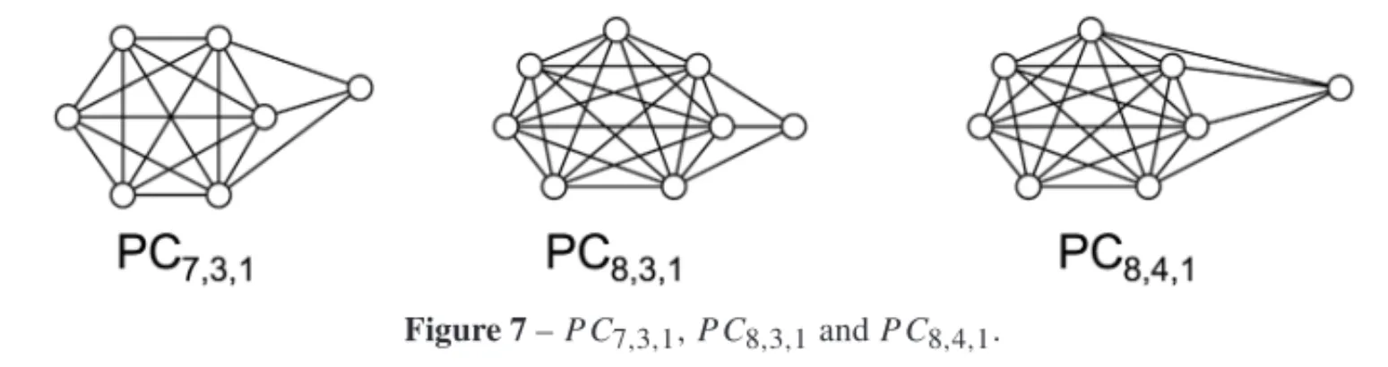
MEASURES OF IRREGULARITY OF GRAPHSFigure 7–P C7,3,1,P C8,3,1andP C8,4,1.
The Figure 7 shows extremal graphs PCn,p,1withn=7 and 8 vertices, whereirr(PC7,3,1)= 18 andirr(PC8,3,1)=irr(PC8,4,1)=24.
Although we still have been unable to determine a simple algebraic expression for the spectral measure even for a small family of graphs such asG = PCn,p,1, we can show some properties of the index of this graph as illustrated in Lemmas 4.1 and 4.2 which can be helpful in the future.
Lemma 4.1. Let n≥4and1≤ p≤n−2. The spectrum of a path complete graph PCn,p,1 is
given by−1with algebraic multiplicity n−3and the remaining eigenvalues are the roots of the following polynomial p(x)=x3+(3−n)x2−(n+p−2)x−2p+np−p2.
Proof. For convenientnandp, the adjacency matrix ofPCn,p,1is as follows:
A(PCn,p,1)=
⎡
⎢ ⎢ ⎣
(J−I)p×p Jp×(n−p−1) Jp×1
J(n−p−1)×p (J−I)(n−p−1)×(n−p−1) O(n−p−1)×1
J1×p O1×(n−p−1) O1×1
⎤
⎥ ⎥ ⎦,
where Jdenotes an all-one-matrix and I is the identity matrix. For 1 ≤i ≤ n, letei ∈Rnbe thei-th vector of the canonical basis. It is not too difficult to see that∀i, 2 ≤ i ≤ n−2, if
v=ei−en−1, thenAv= −v. So,vis an eigenvector correspondent to the eigenvalue−1 with
algebraic multiplicity at leastn−3.
There is an orthogonal basis ofRnformed by the eigenvectors ofA(PCn,p,1). So, there are the eigenvectors asyt =(a,· · ·,a
!
p
,b,· · ·,b
!
n−p−1
,c). Then, the remaining 3 eigenvalues of A(PCn,p,1)
are the same ones of the matrix
B =
⎡
⎢ ⎣
p−1 n−1−p 1
p n−p−2 0
p 0 0
⎤
⎥ ⎦,
which are exactly the roots ofPB(x)=x3+(3−n)x2−nx−(p−2)x−2p+np−p2.
Lemma 4.2.For all p,1≤ p≤n−3, we haveε(PCn,p,1)−ε(PCn,p+1,1)=λ1(PCn,p,1)−
λ1(PCn,p+1,1)+n2.
Proof. It is well known that if H is a subgraph of G, their indices attained the inequality
λ1(H)≤λ1(G). The strict inequality holds ifGis a connected graph andHis a proper subgraph ofG. As PCn,p,1 ⊂ PCn,p+1,1, consequently, for 1 ≤ p ≤ n−3, we haveλ1(PCn,p,1) <
λ1(PCn,p+1,1). LetmPCn,p,1andmPCn,p+1,1be the number of edges of those graphs, respectively. It is obvious thatmPCn,p+1,1 = mPCn,p,1 +1 and, asd(PCn,p,1) =
2mP Cn,p,1
n , we easily have ∀ j, 1 ≤ j ≤ n −3, d(PCn,j+1,1) = d(PCn,j,1)+ n2. So, ε(PCn,p,1)−ε(PCn,p+1,1) =
λ1(PCn,p,1)−λ1(PCn,p+1,1)+2n.
Numerically, with the aid of the software AGX, see [11], we found that the difference between the indices of the graphsPCn,p+1,1 andPCn,p,1is at most 2n. The experiments were done with graphs up ton ≤25 vertices. Based on these, we establish the following conjecture.
Conjecture 4.1.For n≥4and1≤ p≤n−3, we have0< λ1(PCn,p+1,1)−λ1(PCn,p,1) < 2n. From now on we will investigate the irregularity on the complete split graphs.
Definition 4.2.Let k and n be integer numbers such that0 ≤k ≤n. A graph S(n,k)is a split graph if there is a partition of its vertex set into a clique of order k and a stable set of order n−k. A complete split graph, C S(n,k), is a split graph such that each vertex of the clique is adjacent to each vertex of the stable set.
The next two theorems characterize the most irregular complete split graphs relative to
s(C S(n,k)) and irr(C S(n,k)), respectively. As one will see, both extremal graphs are the same. Besides, the theorems show the expression of the respective measures.
Theorem 4.4. Let k ∈ Nand0 ≤ k ≤ n. If G = C S(n,k) is a complete split graph then s(G)= 2nk(n−k)(n−1−k). Besides, among all complete split graphs, the most irregular one by s(G)has to attend the following conditions on k:
k= ⎧ ⎪ ⎪ ⎪ ⎪ ⎪ ⎨
⎪ ⎪ ⎪ ⎪ ⎪ ⎩
n
3, ifnmod(3)=0;
n−1
3 , ifnmod(3)=1;
n−2 3 and
n+1
3 , ifnmod(3)=2.
Proof. ConsiderG=C S(n,k). From the definition of the deviation measure, we haves(G)=
2
nk(n −k)(n −1−k). For a given n, define f(k) = 2
nk(n −k)(n −1−k). The maximal value of f(k)is obtained byk = 23n− 13√n2−n+1−1
3. Sincekis an integer, we have to determine⌈k⌉and⌊k⌋. Let p,r ∈Z+and 0≤r ≤2 such thatn =3p+r. So,n2−n+1=
9p2+6pr+r2−3p−r +1. Letr = 0, and rewriten2−n+1 =9p2−3p+1. Thus,
(3p+1)2−9p=(3p−1)2+3pand 3p−1≤√n2+n−1≤3p+1. Therefore, we reach n
3−1<k≤ n
3 ifnmod(3)=0. Similarly, forr =1 andr =2, we get n−1
3 ≤k< n+2
394
MEASURES OF IRREGULARITY OF GRAPHSFrom the results above, the conditions on⌊k⌋and⌈k⌉follow:
⌊k⌋ = ⎧ ⎪ ⎪ ⎪ ⎪ ⎪ ⎨
⎪ ⎪ ⎪ ⎪ ⎪ ⎩
n
3−1, ifnmod(3)=0;
n−1
3 , ifnmod(3)=1;
n−2
3 , ifnmod(3)=2;
⌈k⌉ = ⎧ ⎪ ⎪ ⎪ ⎪ ⎪ ⎨
⎪ ⎪ ⎪ ⎪ ⎪ ⎩
n
3, ifnmod(3)=0;
n+2
3 , ifnmod(3)=1;
n+1
3 , ifnmod(3)=2.
Finally, after comparing f(⌊k⌋)with f(⌈k⌉)in all previous cases, we reach the following maxi-mal values of f(k),
i) ⌈k⌉ = n
3, if nmod(3)=0; ii) ⌊k⌋ = n−1
3 , if nmod(3)=1 and iii) ⌊k⌋ = n−2
3 and ⌈k⌉ =
n+1
3 , if nmod(3)=2.
The Figure 8 shows extremal graphsC S(n,k)withn =5 and 6 vertices, wheres(C S(5,1) = s(C S(5,2))=4,8 andC S(6,2)=8.
Figure 8–C S(5,1),C S(5,2)andC S(6,2).
Based on the results before and through the several numerical experiments done with the aid of AGX (see [14]), we propose the conjecture below.
Conjecture 4.2.LetH(n)be the set of all connected graphs G with n vertices. So,maxG∈H(n) s(G)=s(C S(n,k))where
k= ⎧ ⎪ ⎪ ⎪ ⎪ ⎪ ⎨
⎪ ⎪ ⎪ ⎪ ⎪ ⎩
n
3, ifn mod(3)=0;
n−1
3 , ifn mod(3)=1;
n−2 3 and
n+1
3 , ifn mod(3)=2.
Theorem 4.5. Let k ∈ N, and0 ≤ k ≤ n. If G = C S(n,k)is a complete split graph, then irr(G)=k(n−k)(n−1−k). Besides, among all complete split graphs, the most irregular one relative to irr(G)has to satisfy the following conditions on k:
k= ⎧ ⎪ ⎪ ⎪ ⎪ ⎪ ⎨ ⎪ ⎪ ⎪ ⎪ ⎪ ⎩ n
3, ifnmod(3)=0;
n−1
3 , ifnmod(3)=1;
n−2 3 and
n+1
3 , ifnmod(3)=2.
Proof. SinceC S(n,k)haskvertices with degreesn−1, andn−kvertices with degreek, we haveirr(G) =k(n−k)(n −1−k). From Theorem 4.4,irr(C S(n,k)) = n2s(C S(n,k)), and
the result holds.
Among all complete split graphs relative to the variance measure, Theorem 4.6 provides the most irregular one.
Theorem 4.6. Let k ∈ Nand0≤ k ≤n. If G =C S(n,k)is a complete split graph, we have σ (SC(n,k)) = 1
n2 (k−n+1) 2(n
−k)k. Besides, among all complete split graphs, the most irregular one relative to s(G)satisfies the following conditions on k:
k= ⎧ ⎪ ⎪ ⎪ ⎪ ⎪ ⎪ ⎪ ⎪ ⎪ ⎨ ⎪ ⎪ ⎪ ⎪ ⎪ ⎪ ⎪ ⎪ ⎪ ⎩ n
4, ifnmod(8)=0 or 4;
n−1
4 , ifnmod(8)=1 or 5;
n−2
4 , ifnmod(8)=2 or 6 and
n+1
4 , ifnmod(8)=3 or 7.
Proof. IfG=C S(n,k), from the definition of the variance measure, we getσ (SC(n,k))= 1 n2 (k−n+1)2(n−k)k. Letnbe given. Define f(k)= 1
n2 (k−n+1) 2(n
−k)k. By elementary algebraic manipulation, we havek=58n−18√9n2−4n+4−1
4as the maximal value to f(k). Similarly the proof of theorem before, the result holds.
Theorem 4.7. The eigenvalues of C S(n,k)are 12(k−1)± 21√4kn−2k−3k2+1 each one
with simple multiplicity; 0 with multiplicity n−k−1and,−1with multiplicity k−1.
Proof. Let J be the all-one-matrix and I be the identity matrix. The adjacency matrix of
C S(n,k)can be written as follows,
A(C S(n,k)) = "
(J−I)k×k Jk×(n−k) J(n−k)×k O(n−k)×(n−k)
#
396
MEASURES OF IRREGULARITY OF GRAPHSFor 2≤i ≤k,v=e1−ei, whereei, is thei-th vector of the canonical basis, is an eigenvector of A(C S(n,k))corresponding to the eigenvalue−1. Its multiplicity is at leastk−1. Besides, note that 0 is an eigenvalue ofA(SC(n,k))to the eigenvectorsx=ej−en,k+2≤ j ≤n. In the last case, its multiplicity is at leastn−k−1. The matrix A(C S(n,k))has an eigenvector with the formyt =(a,· · ·a,
!
k
b,· · ·b ! n−k
). Thus, we conclude that their remaining 2 eigenvalues are
equal to the ones of
B=
"
k−1 n−k
k 0
#
.
Consequently, 12(k−1)±12√4kn−2k−3k2+1 are eigenvalues ofA(C S(n,k)).
From Theorem 4.7, the spectral measure of complete split graphs withnvertices and a clique of sizekis
ε(C S(n,k))= 1
2n(2k−n−3kn+2k
2
+n$4kn−2k−3k2+1).
Although Theorem 4.7 has characterized the eigenvalues to any complete split graph, three of them were implicitly determined. It follows that, the maximum of the spectral measure func-tion is not a simple task. The numerical experiments with done (see [14]) show that, among all connected graphs withnvertices, the complete split graphs are the most irregular to the spectral measure. More specifically, they are the starsSn=C S(n,1), for 4≤n≤11, andC S(n,2), for 12≤n≤15.
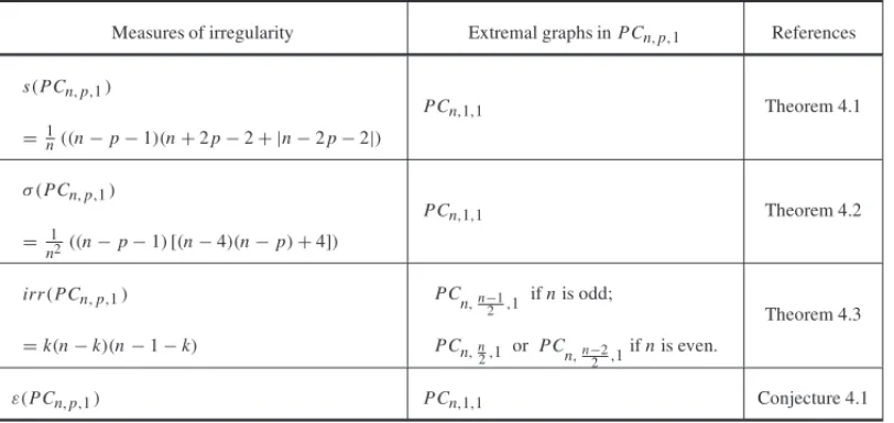
Tables 2 and 3 summarize our results relative to extremalities concerningPCn,p,1andSC(n,k) graphs respectively.
Table 2– The most irregular path complete graphs tos(G),irr(G),σ (G)andε(G).
Measures of irregularity Extremal graphs inPCn,p,1 References
s(PCn,p,1)
= 1n((n−p−1)(n+2p−2+ |n−2p−2|)
PCn,1,1 Theorem 4.1
σ (PCn,p,1)
= n12((n−p−1)[(n−4)(n−p)+4])
PCn,1,1 Theorem 4.2
irr(PCn,p,1)
=k(n−k)(n−1−k)
PCn,n−1 2 ,1
ifnis odd;
PCn,n
2,1 or PCn,n−22,1
ifnis even.
Theorem 4.3
ε(PCn,p,1) PCn,1,1 Conjecture 4.1
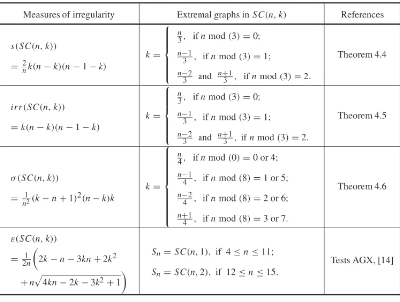
Table 3– The most irregular split complete graphs tos(G),irr(G),σ (G)andε(G).
Measures of irregularity Extremal graphs inSC(n,k) References
s(SC(n,k))
= 2nk(n−k)(n−1−k)
k= ⎧ ⎪ ⎪ ⎪ ⎪ ⎨ ⎪ ⎪ ⎪ ⎪ ⎩ n
3, ifnmod(3)=0; n−1
3 , ifnmod(3)=1; n−2
3 and n+31, ifnmod(3)=2.
Theorem 4.4
irr(SC(n,k))
=k(n−k)(n−1−k)
k= ⎧ ⎪ ⎪ ⎪ ⎪ ⎨ ⎪ ⎪ ⎪ ⎪ ⎩ n
3, ifnmod(3)=0; n−1
3 , ifnmod(3)=1; n−2
3 and n+31,ifnmod(3)=2.
Theorem 4.5
σ (SC(n,k))
= n12(k−n+1)2(n−k)k
k= ⎧ ⎪ ⎪ ⎪ ⎪ ⎪ ⎪ ⎪ ⎪ ⎨ ⎪ ⎪ ⎪ ⎪ ⎪ ⎪ ⎪ ⎪ ⎩ n
4, ifnmod(0)=0 or 4; n−1
4 , ifnmod(8)=1 or 5; n−2
4 , ifnmod(8)=2 or 6; n+1
4 , ifnmod(8)=3 or 7.
Theorem 4.6
ε(SC(n,k))
= 21n %
2k−n−3kn+2k2
+n$4kn−2k−3k2+1 &
Sn=SC(n,1), if 4≤n≤11;
Sn=SC(n,2), if 12≤n≤15.
Tests AGX, [14]
5 CONCLUSION
Among all graphs withnvertices and concerning all the measures of irregularity investigated, the quasi complete graphs are amongst the most irregular ones. However, such an observation is not enough to allow us to identify which irregularity measure is more accurate. Therefore, we have decided to investigate the irregularity in more restricted classes of graphs, such as path complete graphs Pn,p,t (int = 1 cases) and complete split graphs SC(n,k), wherek is the size of the maximal clique of the graph (see Section 4). This investigation allows us to state that:
(i) as it was said before, the imbalance measure does not satisfy the definition of the function
F given in Introduction. In fact, in the particular case of PCn,p,1 graphs, the behavior of the invariantirr(PCn,p,1)does not work as it would be expected (see the third line of Table 2);
(ii) the other three measures,ε(G),s(G)andσ (G), are not comparable. In other words, none of them is more accurate that the other.
ACKNOWLEDGMENTS
398
MEASURES OF IRREGULARITY OF GRAPHSREFERENCES
[1] AHLSWEDER & KATONAGOH. 1978. Graphs with Maximal Number of Adjacent Pairs of Edges. Acta Mathematica Academice Scientiarum Hungaricae,32: 97–120.
[2] ALBERTSONP. 1997. The Irregularity of a graph.Ars Combinatoria,46: 219–225.
[3] AOUCHICHEM, BELLF, CVETKOVIC´D, HANSENP, ROWLINSONP, SIMIKISK & STEVANOVIC´
D. 2008. Variable neighborhood search for extremal graphs. 16. Some conjectures related to the largest eigenvalue of a graph.European Journal of Operational Research,191(3): 661–676.
[4] BELLFK. 1990. On the maximal index of connected graphs.Linear Algebra and its Applications,
161: 45–54.
[5] BELHAIZAS, HANSENP, ABREUNMM & OLIVEIRACS. 2005. Variable Neighborhood Search for Extremal Graphs. XI. Bounds on Algebraic Connectivity. Graph Theory and Combinatorial Opti-mization, Spring, 1–16.
[6] BRANDSTADT¨ A, LEVB & SPINDRADJP. 1999. Graph Classes: a Survey. SIAM Monographs on Dioscrete Mathematics and Applications.
[7] BRUALDIRA & SOLHEIDES. 1986. On the spectral radius of connected graphs.Publications de L’Institut Math´ematique (Beograd) (N.S.),39(53): 45–54.
[8] COLLATZL & SINOGOWITZU. 1957. Spektren endlicher grafen.Abh. Math. Sem. Univ. Hamburg,
21: 63–77.
[9] CVETKOVIC´D & ROWLINSONP. 1988. On connected graphs with maximal index.Publications de L’Institut Math´ematique (Beograd) (N.S.),44(58): 29–34.
[10] HANSENP & M ´ELOTH. 2005. Variable Neighborhood Search for Extremal Graphs 9. Bounding the Irregularity of a Graph.American Mathematical Society,69: 253–264.
[11] HANSENP & CAPOROSSIG. 2000. AutoGraphiX: An Automated System for Finding Conjectures in Graph Theory.Electronic Notes in Discrete Mathematics,5: 158–161.
[12] HARARYF. 1962. The maximum connectivity of graphs.Proc. Nat. Acad. Sci. U.S.A.,48: 1142– 1146.
[13] NIKIFOROVV. 2006. Eigenvalues and degree deviation in graphs.Linear Algebra and its Applica-tions,414: 347–360.
[14] OLIVEIRAJA. 2012. Medidas de Irregularidade em Grafos. Tese de Doutorado, COPPE/UFRJ.