A LAGRANGIAN RELAXATION APPROACH FOR A MACHINERY LOCATION PROBLEM IN FOREST HARVESTING
Jorge R. Vera *
Dept. of Industrial and System Engineering Catholic University of Chile
Santiago – Chile [email protected]
Andrés Weintraub Manfred Koenig Gaston Bravo
Dept. of Industrial Engineering University of Chile
Santiago – Chile
Monique Guignard
Dept. of Operations and Information Management The Wharton School – University of Pennsylvania Philadelphia – USA
Francisco Barahona
IBM Research Center
Yorktown Heights – NY – USA
* Corresponding author / autor para quem as correspondências devem ser encaminhadas Recebido em 04/2002, aceito em 11/2002 após 1 revisão
Abstract
The correct location of harvesting machinery is an important problem for the timber industry, as these are expensive pieces of equipment. Also, access roads need to be constructed within a season of harvesting. In this paper, we present the modelling of this problem as a mixed integer linear model which, without any special technique, is very difficult to solve. Strengthening of the original linear programming formulation, and a Lagrangian Relaxation algorithm are developed to improve the solution process. We show test results in a real industry problem.
1. Introduction
The timber industry around the world has been a longstanding user of Operations Research tools. Many strategic, tactical and operational problems are suited to be modelled as linear programs. Some of these applications have been very successful in certain industrial settings. (See Epstein et al. (1999) for details). In some cases, however, some decisions are of a discrete nature, like harvesting or not harvesting a certain area. This usually requires the models to be of the integer programming kind, with the corresponding additional difficulty on finding a good solution. The problem we present in this paper belongs to this category. It actually involves together a facility location problems as well as a network design problem. Although in practice a feasible solution might be obtainable by mean of heuristic techniques, the knowledge of a good approximation to the optimal value is important, specially for the analysis and calibration of the heuristic techniques.
Specifically, we consider a decision problem which is relevant in the short to medium term, and relates to harvesting operations. In order to harvest a given forest area, it is necessary to install machinery and to build access roads for removing the timber. The machinery consists of harvesting cranes and skidders, with specific operating requirements. The problem fits into an operational framework of decision making in the forest industry. Longer term decisions have already been made, regarding which areas to harvest and when to harvest them. The problem considered here takes these as input and carries out the operational harvesting decisions. This is a complex problem requiring the consideration of several factors, such as installation of harvesting machinery, the area that can be harvested from a given point, and the complexity of the road network which must be built to allow the removal of all the timber. The problem considers only a finite, although large, number of points where machinery can be installed. Roads need to access such points and connect them to demand points. Currently, users at forest companies can use a system called PLANEX (Epstein et al., 1999) to support their decisions. This system is linked to a geographical information system (GIS) which stores information, and in which the forest is represented as a lattice with uniform cells of typically 10 by 10 meters. The information used includes: altitude (topographical level lines), timber availability in each cell, existing roads, type of terrain and topographical accidents such as rivers. An interactive graphical interface allows the user to view the basic data of the problem on screen, as well as the solutions obtained. The user can also modify solutions by proposing alternatives. The solution procedure is based on a heuristic scheme that evaluates all feasible locations of towers and skidders, considering timber that can be reached from it and roads needed for access. Roads are designed based on a shortest path algorithm and data provided by the GIS, where each 10 by 10 cell represents a node in a network. Roads have to satisfy steepness and turning radius constraints. Solutions obtained are naturally only approximate. The system has been implemented in five forest firms in Chile, see Epstein et al. (1999).
with standard strengthening strategies. Coupled with a Lagrangian heuristic, this should provide us with feasible solutions and estimates of the potential error. Our main objective have been to analyze the potential of this approach for a difficult forest management problem and, hence, we have applied the procedure to a real representative forest problem, with promising results.
2. The Forest Problem
In this section we describe the harvesting machinery location problem. Two classes of machinery, towers and skidders are used. A tower is a sort of crane carried by a very heavy truck and placed on top of a hill. Cables are drawn from the crane and anchored at the bottom of the hill, allowing the lifting of timber from the hill side to the top, where it can then be loaded on trucks and transported to the processing plant. At intermediate points, the cable is supported by posts, typically trees are used for this, to keep the cable sufficiently high above the ground. This is to allow for a smooth movement of the logs. After the trees on the hill side and bottom are felled, the cable is laid out at a different angle by moving the bottom end of the cable to a different point from where the harvest can proceed. The cable has a lateral reach for logs of about 30 meters in each direction. This permits the safe harvesting of steep hills in a roughly circular pattern. Cable logging can also be handled downwards, but it is more difficult due to the danger posed by gravity. Skidders are nimble tractors which can move relatively quickly on uneven terrain as long as it is not too steep to carry felled trees to storage areas along roads. Skidders are less expensive to operate than towers. While skidders have flexible mobility, given their low speed, it is considered non economical to have them work long distance, so the road system is designed so that skidders need not carry logs over distances above approximately 300 meters. There are different types of cable logging and skidder machinery, mostly based on reach capacity and cost.
3. The Model
Figure 1 – Harvesting area of a forest. Point A is a machinery location point. The shaded area corresponds to the cells reachable from that location.
B is an intersection of roads and S is the exit of the forest.
We now describe the conceptual model. We assume K different kinds of machinery can be used to harvest wood (although in our application, only two types are used). The cells in the forest are numbered from 1 to n, the C = {1,…,n} will be used to represent them. We will distinguish four subsets of C representing the different kind of cells:
M: set of cells to be harvested.
N: cells representing nodes of the road network.
Tk: set of cells where the operation base of a machine of type, can be installed. We assume that.
S: the set of exit cells. We also assume that S ⊆ N.
We also denote T = ∪kTk. Notice that, with the previous definitions, the cell in N which are neither in T nor in S are intersection of roads.
Associated with the forest there is an undirected graph G = (N,A). A ⊂ N×N describes the roads. These are either potential roads to be built, or already existing road. For that purpose we partition the set of arcs in A = Ae∪ Ap, where Ae corresponds to the already existing roads (eventually Ae = φ), and Ap the potential roads. The following other elements are also used:
Pijk: for machinery of type k, i ∈ Tk and j ∈ M, equals 1if cell j can be harvested from cell i, zero if not. This parameter defines the coverage of a certain machinery location. Ωj: for j ∈ M, timber volume available in cell j.
Kij: A large constant which bounds the flow of timber in road (i,j) ∈ A. αik1
: installation cost for an equipment of type k in cell i ∈ Tk. αij2k
: unit harvesting cost for harvesting with machinery of type k in cell i from cell i ∈ Tk. This is defined only if Pijk = 1.
αqr3: construction cost for road (q,r) ∈ Ap. αqr4
: unit transportation cost for road (q,r) ∈ A.
3.1 Decision Variables
The following variables will be used in the model:
wijk: for j ∈ M, k = 1,…,M, i ∈ Tk, such that Pijk = 1, timber volume at cell j harvested from cell i using machinery of type k.
yi: for i ∈ T, total timber volume harvested through cell i. fqr: timber flow in arc (q,r).
zqr = 1 if we build road (q,r), 0 if not.
xik = 1 if we locate machinery of type k in cell I, 0 if not. gs: timber flow through exit s∈ S.
3.2 Constraints of the Model
• The total timber harvested from one cell cannot be greater than the availability.
1
,
k K
k k
ij ij j
k i T
P w j M
= ∈
≤ Ω ∀ ∈
∑ ∑
(1)• yi equals the sum of all timber amounts harvested through cell i, i ∈ T.
1
,
K
k k
ij ij i
k j M
P w y i T
= ∈
= ∀ ∈
∑ ∑
(2)• Timber can be harvested at cell i from cell j only if some machinery has been installed at i
, , , 1
k k k
ij j i ij
w ≤ Ω x ∀i j k P = . (3)
• There can be traffic on potential road (q,r) (in any direction) only if the road has been built, and road capacity cannot be exceeded:
p ( , ) ,
qr rq qr qr
f +f ≤K z ∀q r ∈A q<r (4)
• There must be flow conservation at harvesting cells, road intersection cell and exit cells.
( , ) ( , )
0 ( )
.
r
qr rt
q r A r t A
r
y r T
f f r N T S g r S
∈ ∈
− ∈
− = ∈ −
∈
∑
∑
∪ (5)• The total timber flowing through the exits should equal the total harvested.
s i
s S i T
g y
∈ ∈
=
∑
∑
(6)• Only one type of machinery can be installed in cell i ∈ T.
1 1,
K k i k
x i T
=
≤ ∀ ∈
∑
(7)3.3 Objective Function
The objective of the model is to harvest the forest by locating equipment, and doing that with maximal benefit. Thus, the objective function considers costs and revenues in the harvesting process. The cost is the sum of the following five terms which accumulate all costs involved in the problem:
• Cost of installing machinery: 1
1 1
K
k ik i k i T
C α x
= ∈
=
∑ ∑
• Harvesting cost:
2 2
1 : 1
α
= ∈ ∈ =
=
∑ ∑ ∑
k ij K
k k ij ij
k i T j M P
C w
• Road construction cost:
p
3 3
( , )
qr qr q r A
C α z
∈
=
∑
• Transportation cost inside the forest: 4
4 ( , )
qr qr q r A
C α f
∈
=
∑
• Transportation cost to final destination: 5
5 s s
s S
C α g
∈
=
∑
• The total revenue for harvesting is:
i i T
y
δ
∈
=
∑
B
The objective function is, thus, to maximize
{
1 … 5}
= − + +
z B C C .
It should be noted that the value of δ can be used to represent actual benefit, or to force, by setting it to a large value, the harvesting of most of the timber in the forest. The computational experiments reported will show that the difficulty of the problem is sensitive to this parameter.
3.4 Difficulty of the Problem and Solution Strategy
1. Defining additional constraints in order to make the original formulation stronger. 2. Partition the problem in the context of a Lagrangian relaxation approach.
3. Strengthen the partitioned subproblems, if possible.
4. Solve the Lagrangian relaxation using a pure subgradient algorithm, or a combined hybrid approach, which consists of subgradient iterations followed by a Dantzig-Wolfe method or by the bundle method.
5. Obtain primal feasible solutions using a Lagrangian heuristic.
The approach we described is justified on the fact that attempting solution of the problem with a simple branch and bound approach leads to excessively large solution times. In fact, as we will see in the computational results, for an instance corresponding to 40 hectares, CPLEX stops after more than 600 minutes only with a feasible solution which gap is 27%. Strengthening can reduce this gap significantly, and the use of a Lagrangian relaxation can provide an even much better bound.
In the following sections of the paper we present the developments of these solution strategies and we finally show some computational results of the approaches in some of our test problems.
4. Strengthening of the Model
It is customary in mixed integer problems to introduce additional constraints that might help in the solution of the problem (see, for example, Wolsey, 1998). These additional relations strengthen the formulation by excluding some fractional solutions. We describe now the improvements we developed for this problem. We first added some constraints to the model. These are redundant for the integer model, but not for its continuous relaxation, thus they could cut off some fractional LP solutions. The constraints we present now are of the “trigger” type based on logical relations between the elements of the model. We also performed an adjustment of the bounds Kij to the maximum possible flow of timber through each arc used in constraints (4).
Location to road triggers: In order to install machinery in a cell, at least one of the roads incident to the corresponding node in the network must be built. The following constraint is generated for each index i ∈ T such that this location is not connected to any existing roads, that is if no q exists such that (i,q) ∈ Ae or (q,i) ∈ Ae:
p p
1 ( , ) ( , )
K k
i iq ri
k i q A r i A
x z z
= ∈ ∈
≤ +
∑
∑
∑
. (8)There are as many of these constraints as location points not connected to existing roads. We do not expect a large number of them, so this does not imply adding an excessive number of constraints to the model.
Road to Road Triggers: These constraints establish that a road cannot exist alone in the network: it has to be connected to others. Let (q,r) ∈ Ap be such that neither q nor r are connected to existing roads. Let us define the set of those arcs by A. Then, the following constraints have to be satisfied by any feasible solution:
p p p p
( , ) ( , ) ( , ) ( , )
, ( , )
qr rt tr qt tq
r t A t r A q t A t q A
z z z z z q r A
∈ ∈ ∈ ∈
Implicit Equations: For all cells which can be harvested from only one cell (that is, Pijk = 1, for only one index i), we can write immediately:
k k
ij j i
w = Ωx . (10)
It is necessary here to make the assumption that if Pijk = 1 then αij2k < δ, that is the unit harvesting cost cannot be greater than the unit revenue.
Capacity Adjustment: To tighten constraints (4), capacities are lowered to the maximum
flow that could go through each road. To determine this value, a preprocessor examines for each road all possible timber flows that might flow through that road. This bound can be quite tight in tree-like network sections, but not so in more dense networks with multiple alternative paths for the flows.
In the computational results we show that these improvements to the model by themselves help in the solution of the problem using a branch and bound algorithm.
5. The Lagrangian Relaxation Idea
The power of commercial mixed-integer programming solvers has improved greatly over the last ten to fifteen years. This is due partly to much faster LP solvers, which allow a much quicker processing of the nodes in the Branch-and-Bound tree. It is also due to the increased use of logical processing and heuristic tools for tightening models and for finding solutions. It remains true, however, that some combinatorial optimization problems are still very difficult to solve by Branch-and-Bound alone. This seems to be the case particularly for problems containing different components that are only loosely connected together by constraints.
obtained from the current solution of the Lagrangian subproblem, is added to the current master problem at each iteration, thus the name constraint generation. The optimal bound is contained in the bracket between the optimal value of the current LP master problem and the value of the best Lagrangian relaxed problem. A composite (hybrid) method, called two-step dual method, was proposed in Guignard & Zhu (1994). In a first phase it updates the multipliers via a subgradient formula, while building a master problem in the background. The estimate of the optimal bound is taken as the optimal value of the current master problem. In the second phase, in order to ensure convergence of the process, it only uses the master problem approach. This approach has proved very successful in optimizing Lagrangian bounds for some problems that could not be handled easily by either of the first two (Guignard & Zhu, 1994). A third approach is the Bundle method. In this approach the past information of subgradients already generated is incorporated into the process, as they already constitute a partial description of the dual function. The rest of the approximation is constructed with a quadratic term. A hybrid method with a bundle approach would start with the subgradient method and shift to the bundle method after an appropriate criteria is satisfied. For details see Hiriart-Urruty & Lemarechal (1993). We tested all three main procedures to solve the Lagrangian relaxation for the problem.
6. Decomposition of the Model
Our problem consists of a machinery location problem, connected to a road construction problem. Given the difficulty in solving the complete problem via Branch-and-Bound techniques, we attempt to separate it into two subproblems using Lagrangian relaxation. We do this by dualizing the constraints that link the two, namely constraints (2). For each one of these constraints a Lagrangean multiplier µi is defined. The corresponding objective function of the relaxed problem is:
1 1 3 4 ( , ) ( , ) ( , , , , , , ) ( ) ( ) p
k k k
i i ik i ij ik i ij
i T i T k k i T j M
ij ij ij ij
i j A i j A
L x y w z f y x P w
z f
λ µ δ µ α α µ
α α ∈ ∈ ∈ ∈ ∈ ∈ = + − − − − −
∑
∑∑
∑∑ ∑
∑
∑
The corresponding relaxed problem is: max ( , , , , , , )
. .
L x y w z f s a
λ µ
,
k
k k
ij ij j
k i T
w P j M
∈
≤ Ω ∀ ∈
∑ ∑
(11), , , 1
k k k
ij i j ij
w ≤ Ωx ∀i j kP = (12)
1 ,
k i k
x ≤ ∀ ∈i T
∑
(13)p , ( , )
rq qr qr qr
f + f ≤z K ∀q r ∈A (14)
( , ) ( , )
0 ( )
∈ ∈ − ∈ − = ∈ − ∈
∑
∑
∪ r qr rtq r A r t A
r
y r T
f f r N T S g r S
i s
i T s S
y g
∈ ∈
=
∑
∑
(16){ }
, 0,1 , 0, 0, 0, 0
x z∈ f ≥ w≥ g≥ y≥
Observe that all constraints appearing in this problem are the same as in the original problem, except that original constraints (2) had been excluded as they were relaxed. Variables x and w in constraints (11), (12) and (13) represent a location problem, while variables f, z, y and g in constraints (14) and (15) represent a network design problem. The problem decomposes in two: one problem involves the location of harvesting machinery, and the other the design of a road network. Both of them are hard problems by themselves, but we expect they can be treated better separately than together in the original formulation. The Lagrangian algorithm will proceed by solving these two problems, and updating the value of the multipliers. We will show in the next sections that by using some heuristic approaches we can reduce considerably the computational effort involved in getting optimal solutions for the subproblems. Also, the algorithm will allow us to obtain, heuristically, feasible solutions to the original problem.
6.1 Strengthening to the Subproblems
The two subproblems are by themselves hard combinatorial optimization problems. The Lagrangian relaxation is applied to the original problem and both subproblems are strengthened independently. Notice that the location to road triggers cannot be used here as they involve both location and road construction variables. However, the implicit equalities (10) are kept.
In the road network design problem, the road to road triggers (9) are kept and two new sets of constraints are added as a way of strengthening the formulation, and replace constraints that are lost in the relaxation. The following constraints:
: =1
≤
∑
Ωk ij
i j
j P
y , (17)
reflect, as constraints (3) did in the original problem, that total inflow to a production origin cannot exceed existing timber volume accessed through that origin. The constraint
i j
i T j M
y
∈ ∈
≤ Ω
∑
∑
(18)is another redundant constraint which is expected to contribute to strengthening the model. The following constraints:
p p
( , ) ( , )
: ≥1 ∈ ∈
≤ +
Ω
∑
∑
∑
kij i
ri it
j r i A i t A
j P
y
z z , (19)
Location Subproblem:
2 1
max ( )
. .
, , , , 1
, 1
1, {0,1}, 0 ,
k
k k k
ij i ij ij ik i
i T j M i T k
k k
ij ij j
k i T
k k k
ij i j ij
k k k
ij i j ij
k i k
P w x
s a
w P j M w x i j k P
w x j M P x i T
x w
µ α α
∈ ∈ ∈
∈
+ −
≤ Ω ∀ ∈
≤ Ω ∀ =
= Ω ∀ ∈ =
≤ ∀ ∈
∈ ≥
∑ ∑
∑ ∑
∑ ∑
∑
Network Design Subproblem:
p p p p
3 4
( , ) ( , )
p
( , ) ( , )
( , ) ( , ) ( , ) ( , )
max ( )
. .
, ( , )
0 ( )
, ( , )
β µ α α
∈ ∈ ∈ ∈ ∈ ∈ ∈ ∈ ∈ ∈ ∈ + − − + ≤ ∀ ∈ − ∈ − = ∈ − ∈ = ≤ + + + ∀
∑
∑
∑
∑
∑
∑
∑
∑
∑
∑
∑
∪i i ij ij ij ij
i T i j A i j A
rq qr qr qr
r
qr rt
q r A r t A
r
i s
i T s S
qr q t A qt t q A tq r t A rt t r A tr
y z f
s a
f f z K q r A y r T
f f r N T S g r S
y g
z z z z z q r
{ }
p p ( , ) ( , ) : 1 : 1 , ,0,1 , 0, 0, 0
∈ ∈ ≥ ∈ ∈ = ∈ ≤ + ∀ ∈ Ω ≤ Ω
≤ Ω ∀ ∈
∈ ≥ ≥ ≥
∑
∑
∑
∑
∑
∑
k ij k ij i ri itr i A i t A
j j P
i j
i T j M
i j P j
A y
z z i T y
y i T
z f y g
7. Implementation of the Solution Approach
solutions of the subproblems, we used a Lagrangian heuristic to obtain another feasible mixed integer solution. We discuss now the specifics of the implementation, basically the criterias used in the Lagrangian relaxation algorithms, and the heuristics used to obtain feasible solutions.
7.1 Implementation of the Lagrangean Approach
Three algorithmic approaches to solve the Lagrangian relaxation were implemented and tested:
1. A basic algorithm based only on pure subgradient iterations.
2. A hybrid method starting with subgradient iterations and shifting to dual Dantzig-Wolf iterations. \item The pure bundle method.
3. A hybrid method starting with subgradient iterations and shifting to the bundle method.
In all cases, the subproblems were solved using Branch and Bound, but all the relevant strengthenings were kept in the subproblems in order to help the search for the optimal solutions. For the subgradient iterations, the stopping criteria was given by having a small tolerance for a given number of iterations.
For the two hybrid approaches, the switching criteria was given by the following rules: 1. when a cut is repeated by the Lagrangian solution, as in Guignard & Zhu (1994). 2. when the optimal value of the master dual problem is under the value of the best
feasible solution.
3. according to a bound on the number of iterations.
4. when the Lagrangian bound does not show significant improvement. In fact, it is typically observed that the convergence of the subgradient iterations is fast at the beginning but no significant improvement is observed in later iterations.
The first criteria to be satisfied triggers the shifting of method. The stopping rule was the same as for the pure subgradient implementation.
The pure bundle approach was less efficient than the hybrid method starting with pure subgradient iterations followed by the bundle method, and these results are not reported.
7.2 Obtaining Feasible Solutions from the Linear Relaxation of the Original Problem
To obtain a feasible solution based on the linear relaxation of the original model, we implemented a simple rounding heuristic which takes the (fractional) values of the location variables and round them in order to make them integer. The road structure is modified in order to guarantee that the locations get connected to the exists. The procedure is as follows:
1. All location variables which are already integer are fixed in their values (zero or one). 2. For the remaining fractional location variables, we test whether the marginal benefit
Criteria 1: Fix variable xik to 1 if
1 2
: 0, 0
( )
α δ α
> >
≤
∑
− Ωk k
ij ij
k
ik ij j
j P w
.
This compares the total installation cost for location i with the additional net benefit obtained from harvesting at that location.
Criteria 2: Fix variable xik to 1 if
1 2
: 0, 0
(1 ) ( )( )
α δ α
> >
− ≤
∑
Ω − −k k
ij ij
k k k
ik i j ij ij
j P w
x w .
This compares the installation cost still to be allocated (the fraction 1 – xik) with the remaining net benefit from harvesting.
If a variable in fractional value does not satisfies neither of the criterias, it is fixed to zero.
3. We then adjust the road network. All road construction variables with positive values are rounded up to value one. The others are kept at value zero. This leaves a road network which connects every location actually used with the exists. We now run the remaining flow problem on the variables (y,w) maximizing net benefits and using the locations and roads already defined by the variable fixing criterias. All roads which end up carrying no flow are eliminated from the solution.
7.3 Obtaining Feasible Solutions from the Lagrangian Relaxation
One of the interesting aspects of Lagrangian Relaxation is the possibility of obtaining feasible solutions to the problem based on the solutions computed from the subproblems, by trying to make them feasible. We developed the following heuristic:
1. If the solution obtained so far is feasible, keep it.
2. If not, it means that the road network is not compatible with the locations defined by the subproblem, which means that some machinery locations are not connected to the exit. The objective is, then, to build up the necessary elements to achieve that connection.
3. We define an auxiliary problem consisting of all machinery locations defined by the location subproblem and an auxiliary road network consisting of a minimum spanning tree connecting all possible machinery locations to the exit. The spanning tree is constructed using a standard algorithm of the Kruskal type (see Ahuja et al., 1993). 4. We solve the auxiliary linear problem to take out all timber to the exits.
5. We eliminate all roads which are not taking any flow of timber.
1. We select all candidate locations to be added to the solution by computing, for candidate location i, the following number:
2 1
: 1
(δ α ) α
=
Ω − −
∑
k ijk k
j ij i
j P
.
This number, if positive, indicates that the total timber harvested at the candidate is enough to compensate the installation cost.
2. After this, the corresponding linear problem is solved again.
3. If the objective does not improve, we eliminate machinery by selecting as candidates all locations corresponding to leafs of the spanning tree. For candidate i we compute
2 1 3
: 0 : 0
(δ α ) α α
> >
Ω − − −
∑
∑
k
ir ij
k k
j ij i ir ir
r f j w
f .
This number, if negative indicates that the transportation cost incurred to take out timber (at least to the immediate roads) is excessive and we should eliminate that installation.
4. We solve the corresponding linear program again.
5. To avoid cycling by examining locations which have been recently considered, we keep a register with that information. This is a sort of tabu list, as used in Tabu Search, a heuristic approach to solve combinatorial optimization problems which has been successful in recent years to tackle difficult problems. (For a detailed discussion, see Glover (1994)). Our local search, however, is not a full implementation of a Tabu Search heuristic and only a few iterations for improvement are performed.
8. An Alternative Formulation
An alternative formulation of the problem is obtained by realizing that the constraints (3): , , , 1
k k k
ij j i ij
w ≤ Ω x ∀i j k P =
can be replaced by one for each location by adding in the index j. The constraint
: 1 : 1
,
= =
≤ Ω ∀ ∈
∑
∑
k k
ij ij
k k
ij i j
j P j P
w x i T (20)
is an aggregation of the above and if included instead of them provides a more compact representation of the model. In fact, for large size problems, most of the constraints in the original model are of the type (3). Replacing them by (20) implies only one constraint for each potential machinery location point. This formulation, however, since it is less tight, proved to be less powerful for solving the problem using Branch and Bound, although the linear relaxation could be solved faster as there are less constraints.
solution. We then add to the problem the corresponding disaggregated constraints only for the indexes (i,j) that satisfies the above criteria. This approach, however, did not provide better solutions at reasonable CPU time compared with the use of the full set of constraints (3), and these tests are not reported.
9. Computational Results
9.1 Test Problems
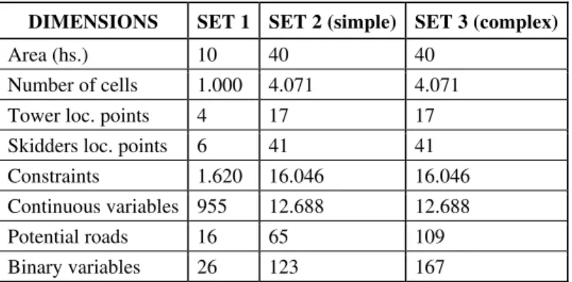
We tested the algorithms on two different data sets. The first one represents a small problem. The second one corresponds to a larger problem and it is based on real data from a plantation. For this problem we generated two different cases based on different structures of the network of potential roads. We did this to test the robustness of the algorithm to changes in the structure of the network. In the first case we generated a simplified structure consisting on a spanning tree connecting all location points, together with the existing roads. For the second case, we used the original network of potential roads available from the original data, which is substantially more complex than a spanning tree. Table 1 summarizes the characteristics of both instances. We also generated different instances based on a different value for the benefit obtained from harvesting, in order to test for the sensitivity of the approach to changes in market conditions.
Table 1 – Description of the test problems
DIMENSIONS SET 1 SET 2 (simple) SET 3 (complex) Area (hs.) 10 40 40
Number of cells 1.000 4.071 4.071 Tower loc. points 4 17 17 Skidders loc. points 6 41 41
Constraints 1.620 16.046 16.046 Continuous variables 955 12.688 12.688
Potential roads 16 65 109 Binary variables 26 123 167
9.2 Results of the Runs
We performed testing of the algorithms developed using both instances presented in the previous section. For each instance, we first solved the linear relaxation of the original problem, and applied the rounding heuristic described in 5.3 We then attempted to solve the problem using a Branch & Bound procedure. This was successful only for the small problem and for the large one only with the simple road structure. We then applied the Lagrangian relaxation, in its three different implementations, to the problem, using the Lagrangian heuristic to obtain a feasible solution.
Table 2 – Results for δ = 18
INSTANCE Linear Relaxation Branch & Bound Lagrangian relaxation normal strengthened normal strengthened Subgradient Hibrid Bundle
SET 1
Feas. sol. 9,341 9,687 10,704 10,704 10,704 10,704 10,704 Bound 14,299 11,785 10,704 10,704 11,423 11,281 11,281 Gap (%) 34.7 17.8 0.0 0.0 6.3 5.1 5.1
Time (min) 0.05 0.03 1.50 0.75 2.36 2.96 2.334
SET 2
Feas. sol 81,857 86,411 83,989 91,888 90,546 91,542 91,542 Bound 105,911 102,321 99,875 91,888 101,321 97,512 96,524 Gap (%) 22.7 15.5 15.9 0.0 10.6 6.1 5.2
Time (min) 8.63 10.23 600.28 29.18 150.31 165.12 143.34
SET 3
Feas. sol 70,776 81,475 76,125 91,888 92,056 * * Bound 106,227 101,5554 104,278 98,765 97,890 Gap (%) 33.4 19.8 27.0 7.0 6.0
Time (min) 10.30 12.54 632.14 629.18 340.45
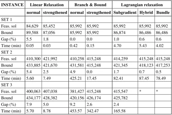
Table 3 – Results for δ = 50
INSTANCE Linear Relaxation Branch & Bound Lagrangian relaxation normal strengthened normal strengthened Subgradient Hybrid Bundle
SET 1
Feas. sol 84,629 85,452 85,992 85,992 85,992 85,992 85,992 Bound 89,588 87,056 85,992 85,992 86,874 86,486 86,486
Gap (%) 5.5 1.8 0.0 0.0 1.0 0.6 0.6
Time (min) 0.05 0.03 0.42 0.15 4.70 5.43 4.02
SET 2
Feas. sol 410,300 421,992 410,258 415,248 414,259 415,248 415,248 Bound 433,885 421,670 431,581 415,248 421,345 418,123 417,253
Gap (%) 5.4 2.5 4.9 0.0 1.7 0.7 0.5
Time (min) 5.60 7.49 425.21 17.45 82.41 87.45 78.49
SET 3
Feas. sol 400,063 407,038 381,427 415,248 415,547 * * Bound 434,177 428,382 420,156 426,174 425,782
Gap (%) 7.9 5.0 9.2 2.6 2.4
Several conclusions are obtained from the results. First, the fact that the problem is hard is reflected in that the Branch and Bound algorithm was not able to solve the basic formulation in a reasonable time, except in the small instance. However, a significant improvement is obtained by strengthening the formulation of the model. This benefits both the straightforward use of Branch and Bound, and the Lagrangian relaxation. Notice that the Branch and Bound leads to significantly lower gaps, in particular for the higher benefit cases, but at the cost of higher CPU times compared to the Linear Relaxation approach. The larger problem with complex road structure is harder to solve. In the Lagrangian relaxation approach we have the following conclusions:
1. The hybrid method with bundle iterations appears slightly better than the hybrid combined with Dantzig-Wolfe iterations, and both are better than the pure subgradient approach.
2. For the most difficult problem (large instance with complex road structure), the algorithm did not reach the shifting stage in the hybrid method and only subgradient iterations were performed.
3. The Lagrangian approach appears worse for the easier problems.
In fact, the linear relaxation of the problem, when those constraints are added shows an improvement of the gap, for the linear relaxation of the large problem with complex structure, from the order of 30% to the order of 20%, in an acceptable time. Moreover, the Branch and Bound procedure greatly benefits from the additional constraints, as can be seen from the tables. A gap of 27.0% without strengthening reduces to 7.0% with them, for the same order of computation time. Finally, the Lagrangian Relaxation also takes advantage of this. The main conclusion of the results is that the Lagrangian procedure can achieve a slightly smaller gap than the best Branch and Bound but, roughly in one half of the time. We can also see from the results that a simpler road structure definitely favors the performance of the algorithm. Also the benefit associated to harvesting has an important effect. This is explained by the fact that a large benefit translates into a much larger importance of the cost coefficient associated to the continuous variables of the problem. This favors the faster computation of a good approximation.
10. Conclusions
the easier problems, but was superior for the more difficult medium sized, dense network, leading to slightly smaller gap in about one third of the CPU time.
As conclusion we note that strengthening of the formulation does significantly improve the solutions process, and Lagrangian relaxation seems to be a promising approach for larger, more difficult to solve problems. It also provides a method to obtain a bound on the objective for the purpose of evaluating heuristic procedures. But, in the few test cases carried out, the proposed approach appears to not be able to tackle larger, dense network problems successfully. More extensive testing is required to achieve clear conclusions on the applicability of Lagrangian relaxation, but this preliminary study suggests that the approach is promising, specially if it is combined with strengthening procedures.
Acknowledgments
Research partially supported by FONDEF, under project FI-11, NSF grant DDM-9014901 and INT93-14779, and FONDECYT under project 1000959.
References
(1) Ahuja, R.; Magnanti, T. & Orlin, J. (1993). Network Flows: Theory, Algorithms and Applications. Prentice Hall.
(2) Fisher, M.L. (1985). An Application Oriented Guide to Lagrangean Relaxation. Interfaces, 15, 10-21.
(3) Epstein, R.; Morales, R.; Serón, J. & Weintraub A. (1999). OR Models in the Chilean Forest Industry. Interfaces, 29, 7-26.
(4) Everett III, H. (1963). Generalized lagrangean Multiplier Method for Solving Problems of Optimum Allocation of Resources. Operations Research, 2, 399-417.
(5) Geoffrion, A.M. (1974). Lagrangean Relaxation for Integer Programming. Mathematical Programming Study, 2, 82-114.
(6) Glover, F. (1994). Tabu Search: Improved Solution Alternatives. In: Mathematical Programming, State of the Art, University of Michigan, 64-92.
(7) Guignard, M. & Zhu, S. (1994). A Hybrid Algorithm for Solving Lagrangean Duals in Mixed Integer Programming. Technical report, The Wharton School, University of Pennsylvania.
(8) Held, M. & Karp, R. (1970). The Travelling Salesman Problem and Minimum Spanning Trees. Operations Research, 18, 1138-1162.
(9) Hiriart-Urruty, J.B. & Lemarechal, C. (1993). Convex Analysis and Minimization Algorithms II: Advanced Theory and Bundle Methods. Springer.
(10) Weintraub, A. & Epstein, R. (1995). PLANEX: A System for the Short term location of forest machinery. Proceedings of the LIRO Conference on Harvest Planning, Nelson, New Zealand, Nov. 1995.