Cost-effective on-demand associative author name disambiguation

Cost-effective on-demand associative author name disambiguation

Adriano Veloso, Anderson A. Ferreira, Marcos André Gonçalves

⇑

_{, Alberto H.F. Laender,}

Wagner Meira Jr.

Departamento de Ciência da Computação, Universidade Federal de Minas Gerais, Brazil

a r t i c l e

i n f o

Article history: Received 8 April 2010

Received in revised form 9 August 2011 Accepted 12 August 2011

Available online 1 October 2011

Keywords: Machine learning Digital libraries

Author name disambiguation Associative methods Lazy strategies

a b s t r a c t

Authorship disambiguation is an urgent issue that affects the quality of digital library ser-vices and for which supervised solutions have been proposed, delivering state-of-the-art effectiveness. However, particular challenges such as the prohibitive cost of labeling vast amounts of examples (there are many ambiguous authors), the huge hypothesis space (there are several features and authors from which many different disambiguation func-tions may be derived), and the skewed author popularity distribution (few authors are very prolific, while most appear in only few citations), may prevent the full potential of such techniques. In this article, we introduce an associative author name disambiguation approach that identifies authorship by extracting, from training examples, rules associating citation features (e.g., coauthor names, work title, publication venue) to specific authors. As our main contribution we propose three associative author name disambiguators: (1) EAND (Eager Associative Name Disambiguation), our basic method that explores associa-tion rules for name disambiguaassocia-tion; (2) LAND (Lazy Associative Name Disambiguaassocia-tion), that extracts rules on a demand-driven basis at disambiguation time, reducing the hypoth-esis space by focusing on examples that are most suitable for the task; and (3) SLAND (Self-Training LAND), that extends LAND with self-training capabilities, thus drastically reducing the amount of examples required for building effective disambiguation functions, besides being able to detect novel/unseen authors in the test set. Experiments demonstrate that all our disambigutators are effective and that, in particular, SLAND is able to outperform state-of-the-art supervised disambiguators, providing gains that range from 12% to more than 400%, being extremely effective and practical.

Ó_{2011 Elsevier Ltd. All rights reserved.}

1. Introduction

Citations (here understood as a set of bibliographic features such as author and coauthor names, work title and pub-lication venue title, of a particular pubpub-lication) are an essential component of many current digital libraries (DLs) and sim-ilar systems (Lee, Kang, Mitra, Giles, & On, 2007). Citation management within DLs involves a number of tasks. One task in particular, name disambiguation, has required significant attention from the research community due to its inherent dif-ficulty. Name ambiguity in the context of bibliographic citations occurs when one author can be correctly referred to by multiple name variations (synonyms) or when multiple authors have exactly the same name or share the same name var-iation (polysems). This problem may occur for a number of reasons, including the lack of standards and common practices, and the decentralized generation of content (e.g., by means of automatic harvesting).

0306-4573/$ - see front matterÓ2011 Elsevier Ltd. All rights reserved. doi:10.1016/j.ipm.2011.08.005

⇑ Corresponding author. Tel.: +55 31 34095860; fax: +55 31 34095858. E-mail address:mgoncalv@dcc.ufmg.br(M.A. Gonçalves).

Contents lists available atSciVerse ScienceDirect

Information Processing and Management

The name disambiguation task may be formulated as follows. LetC= {c1,c2,. . .,ck} be a set of citations. Each citationcihas

a list of attributes which includes at least author names, work title and publication venue title. The objective is to produce a disambiguation function which is used to partition the set of citations intonsets {a1,a2,. . .,an}, so that each partitionai

con-tains (all and ideally only all) the citations in which theith author appears.

To disambiguate the bibliographic citations of a digital library, first we may split the set of citations into groups of ambig-uous authors, called ambigambig-uous groups (i.e., groups of citations having authors with similar names). The ambigambig-uous groups may be obtained, for instance, by using a blocking method (On, Lee, Kang, & Mitra, 2005). Blocking methods address scala-bility issues, avoiding the need for comparisons among all citations.

The complexity of dealing with ambiguous names in DLs has led to myriad of methods for name disambiguation (Bhattacharya & Getoor, 2006, 2007; Culotta, Kanani, Hall, Wick, & McCallum, 2007; Han, Giles, Zha, Li, & Tsioutsiouliklis, 2004; Han, Xu, Zha, & Giles, 2005; Han, Zha, & Giles, 2005; Huang, Ertekin, & Giles, 2006; Malin, 2005; On et al., 2005; Song, Huang, Councill, Li, & Giles, 2007; Torvik & Smalheiser, 2009; Cota, Ferreira, Nascimento, Gonçalves, & Laender, 2010). Some of the most effective methods seem to be based on the application of supervised machine learning techniques. In this case, we are given an input data set called thetraining data(denoted asD) which consists of examples, or, more specifically, citations for which the correct authorship is known. Each example is composed of a set of mfeatures (f1,f2,. . .,fm) (e.g.,

corresponding to coauthor names or words in titles) along with a special variable called theauthor. Thisauthorvariable draws its value from a discrete set of labels (a1,a2,. . .,an), where each label uniquely identifies an author. The training data

is used to produce a disambiguator that relates the features in the training data to the correct author. Thetest set(denoted as

T) for the disambiguation problem consists of a set of citations for which the features are known while the correct author is unknown. The disambiguator, which is a function from {f1,f2,. . .,fm} to {a1,a2,. . .,an}, is used to predict the correct author of

citations in the test set.

Although successful cases have been reported (Han et al., 2004; Han, Xu, et al., 2005; Torvik & Smalheiser, 2009), some particular challenges associated with author name disambiguation (in the context of bibliographic citations), prevent the full potential of supervised machine learning techniques:

The acquisition of training examples requires skilled human annotators to manually label citations. Annotators may face hard-to-label citations with highly ambiguous authors. The cost associated with this labeling process thus may render vast amounts of examples unfeasible. The acquisition of unlabeled citations, on the other hand, is relatively inexpensive. However, it may be worthwhile annotating at least some examples, provided that this effort will be then rewarded with an improvement in disambiguation effectiveness. Thus, disambiguators must be cost-effective, achieving high effective-ness even in the case of limited labeling efforts.

There is a potentially large number of features and authors, and consequently, the number of possible disambiguation functions that may be derived from them is huge. Selecting an appropriate function, given so many possibilities, is chal-lenging. Thus, disambiguators must focus on producing only functions that are suitable to disambiguate specific citations.

The number of citations in which a particular author is included is extremely skewed. Specifically, few authors are very popular, appearing in several citations, while most of the authors publish only few papers. The effective disambiguation of less popular authors is particularly challenging, since, in such cases, only few examples are available for building a dis-ambiguation function. On the other hand, this is particularly important, because these authors, collectively, may appear in the majority of the citations. Thus, disambiguators must exploit all available evidence, even if such evidence is associated with rarely appearing authors.

It is not reasonable to assume that all possible authors are included in the training data (specially due to the scarce avail-ability of examples). Thus, disambiguators must be able to detect unseen/unknown authors, for whom no label was pre-viously specified.

There are countless strategies for devising a name disambiguator for bibliographic citations. One of these strategies is to exploit dependencies and associations between bibliographic features and authors. These associations are usually hidden in the examples and, when uncovered, they may reveal important aspects concerning the underlying characteristics of each author (i.e., typical coauthors, typical publication venues, writing patterns, and any combination of these aspects). Obviously, these aspects are evidence that may be exploited for the sake of predicting the correct author of a citation. This is the strategy adopted by associative disambiguators, where the disambiguation function is built from rules of the formX !ai(whereXis

a set of features andaiis an author label). Exploiting associations hidden in examples has shown to be valuable in many

applications, including ranking (Veloso, Mosrri, & Gonçalves, 2008), and document categorization (Veloso, Cristo, Gonçalves, & Zaki, 2006).

EAND, which works in a eager manner, provides the basic foundations for the use of association rules for name disambiguation.

LAND extracts rules from the examples on a demand-driven basis, according to the citation being disambiguated. Thus, instead of producing a single disambiguation function that is good on average (considering all citations in the test set), LAND follows a lazy strategy that delays the inductive process until a citation is given for disambiguation. Then, a specific disambiguation function is produced for that citation. This citation-centric strategy ensures that evidence coming from citations belonging to less popular authors are not neglected during rule extraction. Thus, this strategy is specially well suited for ambiguous groups where the popularity distribution of authors is skewed. Further, extracting rules on a demand-driven basis also reduces the hypothesis space, since there is a concentration on extracting only rules that are relevant to the specific citation being considered.

To limit labeling efforts (which is a major problem in real world scenarios), SLAND extends LAND by employing a self-training strategy, in which a reliable prediction is considered as a new example and is included in the self-training data. Since rules are extracted on a demand-driven basis, at disambiguation time, the next citation to be processed will possibly take advantage of the recently included (pseudo-)example.

SLAND uses the lack of enough evidence (i.e., rules) supporting any known author present in the training data, to detect the appearance of a novel/unseen author in the test set. In such case, a new label is associated with this novel author, and the corresponding citation is considered as a new example which is included in the training data.

The proposed associative disambiguators are intuitive (easily understood using a set of illustrative examples), and also extremely effective, as it will be shown by a systematic set of experiments using citations extracted from the DBLP1_and BDB-Comp2_{collections. The results show that, while EAND is in close rivalry with previously representative supervised} disambigu-ators, LAND is able to outperform all of them with gains in terms of macroF1of more than 12%. Improvements reported by SLAND are also impressive, showing the advantages of its self-training ability specially when there is a scarce availability of examples.

The rest of this article is organized as follows. Section2discusses related work. Section3introduces our associative name disambiguation approach and the three new disambiguators and their properties in details. Section4presents our experi-mental evaluation. Finally, Section5concludes the article with some discussion about future work.

2. Related work

Existing name disambiguation methods adopt a wide spectrum of solutions that range from those based on supervised learning techniques (Han et al., 2004) to those that use some unsupervised or semi-supervised strategy (Bhattacharya & Getoor, 2006, 2007; Culotta et al., 2007;Han, Xu,et al., 2005;Han, Zha, & Giles, 2005;Huang et al., 2006; On et al., 2005; Song et al., 2007; Torvik, Weeber, Swanson, & Smalheiser, 2005) or follow a graph-oriented approach (Malin, 2005; On & Lee, 2007; On, Elmacioglu, Lee, Kang, & Pei, 2006). In this section, we present a brief review of some representative author name disambiguation methods. Our main focus, however, is on those methods that have been specifically designed for addressing the author name disambiguation problem in the context of bibliographic citations, since they are more related to the scope of our work.

Being some of the first to address the problem,Han et al. (2004)propose two methods based on supervised learning tech-niques that use coauthor names, work titles and publication venue titles as evidence for name disambiguation. The first method uses a naive Bayes model to capture all writing patterns in the authors’ citations whereas the second method is based on Support Vector Machines (SVMs). Both methods have been evaluated using two collections, one from the Web (mainly publication lists from homepages), and the other from DBLP.

InHan, Zha, et al. (2005), the authors propose an unsupervised method for name disambiguation that uses k-way spectral clustering. This method was also evaluated with collections extracted from the Web and from DBLP. The results showed that this method has achieved 63% of accuracy in the collection extracted from DBLP, and 71.2%, and 84.3% of accuracy in the collections extracted from the Web.

In Torvik et al. (2005), the authors propose a probabilistic metric for determining the similarity between MEDLINE records. The learning model is created using similarity profiles between articles. A similarity profile is a comparison vector between a pair of articles, used to indicate the similarity between them, based on the following attributes: work title, pub-lication venue title, coauthor and author names, medical subject headings, language, and affiliation. The authors also propose some heuristics for generating training sets (positive and negative) automatically. When the probabilistic metric receives two records, their similarity profile is computed and the relative frequency of this profile in the positive and negative train-ing sets is checked for determintrain-ing whether these two records are authored by the same author or not. InTorvik and Smalhe-iser (2009), the authors extend their method including the addition of new features, new ways of automatically generating training sets, an improved algorithm for correcting the transitivity problem, and a new agglomerative clustering algorithm.

On et al. (2005)present a comparative study of disambiguation strategies based on a two-step framework. In the first step (blocking), similar names are blocked together in order to reduce the number of candidates for the second step (disambig-uation), which uses coauthor information to measure the distance between two names in the citations.

On et al. (2006)then propose a graph-based method for disambiguation that uses a graph in which each vertex represents an author and each edge represents a coauthorship between two authors. After ambiguous groups are determined, the meth-od finds the common quasi-clique between two vertices and the vertex degree of this quasi-clique is used as a similarity measure for the respective authors. Results expressed in terms of average ranked precision measures, considering real and synthetic collections, have shown that this method considerably improves the effectiveness of traditional text similarity measures.

Huang et al. (2006)present a framework for name disambiguation in which a blocking method first creates candidate classes of authors with similar names and then DBSCAN, a density-based clustering method (Ester, Kriegel, Sander, & Xu, 1996), is used to cluster citations by author. For each block, the distance metric between citations used in DBSCAN is calculated by an online active selection SVM, which yields, according to the authors, a simpler model than those obtained by standard SVMs. This method exploits additional sources of evidence, such as information extracted from the headers of papers corresponding to the respective citations obtained from CiteSeer.

InBhattacharya and Getoor (2006), the authors extend the Latent Dirichlet Allocation model and propose a probabilistic model for collective entity resolution that uses the cooccurrence of the references to entities3_{in each work to determine the} entities jointly, i.e., they use the disambiguated references to disambiguate other references in the same work. An algorithm for collective entity resolution that uses the attributes and relational information of the citation records is proposed in (Bhattacharya & Getoor, 2007).

Culotta et al. (2007)propose a more generic representation for the author disambiguation problem that considers fea-tures over sets of records, instead of only feafea-tures between pairs of records, and present a training algorithm that is er-ror-driven, i.e., training examples are generated from incorrect predictions in the training data, and rank-based, i.e., the classifier provides a ranked result for the disambiguation. Whereas in (Kanani, McCallum, & Pal, 2007), the authors present several methods for increasing the author coreference by gathering additional evidence from the Web.

Cota, Gonçalves, and Laender (2007, 2010)propose a heuristic-based hierarchical clustering method for name disambig-uation that involves two steps. In the first step, the method creates clusters of citations with similar author names. Then, in the second step, the method successively fuses clusters of citations with similar author names based on several heuristics. In each fusion, the information of fused clusters is aggregated, providing more information for the next round of fusion. This process is successively repeated until no more fusions are possible.

On and Lee (2007)have studied the scalability issue of the disambiguation problem. They examine two state-of-the-art solutions, k-way spectral clustering (Han, Zha, et al., 2005) and multi-way distributional clustering (Bekkerman & McCallum, 2005), and pointed out their limitations with respect to scalability. Then, using collections extracted from the ACM DL and from DBLP, they showed that a method based on the multi-level graph partition technique (Dhillon, Guan, & Kulis, 2005) may be successfully applied to name disambiguation in large collections.

InSong et al. (2007), the authors propose a two-step unsupervised method. The first step, after learning the probability distribution of the title and publication venue words and author names, uses Probabilistic Latent Semantic Analysis and La-tent Dirichlet Allocation to assign a vector of probabilities of topics to a name. In the second step, they consider the prob-ability distribution of topics with respect to person names as new evidence for name disambiguation.

Kang et al. (2009)explore the use of coauthorship using a Web-based technique that obtains implicit coauthors of the author to be disambiguated. They submit as query a pair of citation author names to Web search engines to retrieval doc-uments that contains both author names, and to extract the new names found in these docdoc-uments as new implicit coauthors of the pair.

Pereira et al. (2009)also exploit the Web for obtaining additional information to disambiguate author names. The pro-posed method attempts to find Web documents corresponding to curricula vitae or Web pages containing publications of a single author. If two citations of two ambiguous authors occur in the same Web document, these citations are considered as belonging to the same author and are fused in a same cluster. One problem with this method and the previous one is the additional cost of extracting all the needed information from Web documents.

Finally,Treeratpituk and Giles (2009)propose a pairwise linkage function for author name disambiguation in the Medline digital library. The authors exploit a large feature set obtained from Medline metadata, similar to that of (Torvik et al., 2005), and assess the effectiveness of random forests, in comparison to other classifiers, for constructing a pairwise linkage function to be used in some author name disambiguation algorithms. They also investigate subsets of the features capable of reaching good effectiveness.

Since name disambiguation is not restricted to a single context, it is worth noting that several other disambiguation methods, which exploit distinct sources of evidence or are targeted to other applications. For instance,Malin (2005)propose two methods for name disambiguation that exploit the existing relations among ambiguous names. The first method is based on a hierarchical clustering strategy and the second one makes use of social networks.Vu, Masada, Takasu, and Adachi (2007) propose the use of Web directories as a knowledge base to disambiguate personal names in Web search results,

whereasBekkerman and McCallum (2005)present two methods for addressing this same problem, one based on the link structure of Web pages, the other one using agglomerative/conglomerative double clustering, a multi-way distributional clustering. A deeper discussion of these methods, however, are out of the scope of this paper.

Despite all such efforts, problems due to the huge hypothesis space and the skewed popularity distribution of authors are often neglected. Further, another difficulty is imposed by practical constraints, which may render vast amounts of examples unfeasible. All these problems may prevent the full potential of supervised disambiguation methods. Thus, addressing these problems is an opportunity for improvement, and is the target of our study.

3. Associative disambiguation

Associative name disambiguation, in the context of bibliographic citations, exploits the fact that, frequently, there are strong associations between bibliographic features (f1,f2,. . .,fm) and specific authors (a1,a2,. . .,an). Here, we consider as

fea-ture each coauthor name and each word in work or publication venue titles. The learning strategy adopted by associative disambiguators is based on uncovering such associations from the training data, and then building a function

{f1,f2,. . .,fm}?{a1,a2,. . .,an} using such associations. Typically, these associations are expressed using rules of the form

X !a1;X !a2;. . .;X !an, whereX#ff1;f2;. . .;fmg. For example, {coauthor=K.Talwar,title=Metric,venue=LATIN}?a1

while {coauthor=W.Lin,title=Optimal,title=Sparse}?a2are two association rules indicating that the coauthor name ‘‘K. Talkar’’, the word ‘‘Metric’’ in the work title and ‘‘LATIN’’ in the publication venue title are associated with the authora1 (Anupam Gupta) and the coauthor name ‘‘W. Lin’’ and the words ‘‘Optimal’’ and ‘‘Sparse’’ in the work title are associated with the authora2(Chuen-Liang Chen).

In the following discussion we will denote asRan arbitrary rule set. Similarly, we will denote asRaia subset ofRwhich

is composed of rules of the formX !ai(i.e., rules predicting authorai). A ruleX !aiis said to match citationxifX#x(i.e.,x

contains all features inX), and these rules form the rule setRx

ai. That is,R x

ai is composed of rules predicting authoraiand

matching citationx. Obviously,Rx

ai#Rai#R.

Naturally, there is a total ordering among rules, in the sense that some rules show stronger associations than others. A widely used statistic, called confidence (Agrawal, Imielinski, & Swami, 1993) (denoted ashðX !aiÞÞ, measures the strength

of the association betweenXandai. The confidence of the ruleX !aiis simply calculated by the conditional probability ofai

being the author of citationx, given thatX#x.

Using a single rule to predict the correct author may be prone to error. Instead, the probability (or likelihood) ofaibeing

an author of citationxis estimated by combining rules inRx

ai. More specifically,R x

aiis interpreted as a poll, in which each rule

X !ai2 Rxaiis a vote given by features inXfor authorai. The weight of a voteX !aidepends on the strength of the

asso-ciation betweenXandai, which ishðX !aiÞ. The process of estimating the probability ofaibeing the author of citationx

starts by summing weighted votes foraiand then averaging the obtained value by the total number of votes forai, as

ex-pressed by the score functions(ai,x) shown in Eq.(1)(whererj#RxaiandjR x

aijis the number of rules inR x

ai). Thus,s(ai,x) gives

the average confidence of the rules inRx

ai(obviously, the higher the confidence, the stronger the evidence of authorship).

sðai;xÞ ¼ PjRxaij

j¼1hðrjÞ

jRx aij

ð1Þ

The estimated probability ofaibeing an author of citationx, denoted as^pðaijxÞ, is simply obtained by normalizings(ai,x),

as shown in Eq.(2). A higher value of^pðaijxÞindicates a higher likelihood ofaibeing an author ofx. The author associated

with the highest likelihood is finally predicted as the correct author of citationx.

^

pðaijxÞ ¼

sðai;xÞ Pn

j¼1sðaj;xÞ ð2Þ

Next, we will introduce novel associative name disambiguators: EAND, LAND, and SLAND. We will start by discussing EAND, since it is the simplest disambiguator. Then, we will discuss LAND, which employs a more sophisticated rule extrac-tion strategy. Lastly, we will SLAND, which extends LAND, being less sensitive to scarce training and the presence of new authors.

3.1. Eager Associative Name Disambiguation

Rule extraction is a major issue when devising an associative disambiguator. Extracting all rules from the training data is infeasible and, thus, pruning strategies are employed in order to reduce the number of rules that are processed. A simple pruning strategy is based on a support threshold,

r

min, which separates frequent from infrequent rules. This is the strategy

adopted by EAND, the Eager Associative Name Disambiguator that will be presented in this section.

The

r

minthreshold produces a minimum cut-off value,

p

min, as shown in Eq.(3)(whereceil(z) is the nearest integer

great-er than or equal toz).

The number of citations in the training data in which ruleX !aihas occurred is denoted as

p

ðX !aiÞand this rule is

frequent if it is supported by at least

p

min citations in the training data (i.e.,

p

ðX !aiÞP

p

min). Ideally, infrequent rules

are not important. However, most of the authors appear in very few citations and, thus, rules predicting such authors are very likely to be infrequent and, consequently, they are not included inR. These infrequentfeature-authorassociations may be important for the sake of disambiguation and, therefore, disambiguation effectiveness is seriously harmed when such rules are pruned.

Algorithm 1. Eager Associative Name Disambiguation.

Require: Examples inD;

r

min, and citationx2 T

Ensure: The predicted author of citationx

1:

p

min(

r

min jDj

2:R (rulesrextracted fromDj

p

ðrÞP

p

_min 3:for eachauthoraido

4: Rx

ai(rulesX !ai2 Rj

p

ðX !aiÞP

p

minandX#x

5: Estimate^pðaijxÞ, according to Eq.(2)

6:end for

7: Predict authoraisuch that^pðaijcÞ>^pðajjcÞ8j–i

A naive solution is to lower the value of

r

min, so that rules predicting less popular authors are also included inR. This

solution, however, may be disastrous as the amount of rules that are processed may increase in a very large pace (a problem known as rule explosion). Even worse, most of these rules are useless for the sake of disambiguation.4_{An optimal value of}

r

minis unlikely to exist, and tuning is generally driven by intuition and prone to error as a consequence. The main steps of EAND

are shown inAlgorithm 1. There is a vast amount of association rule mining algorithms (Goethals & Zaki, 2004) and we assume that any of these algorithms can be used (or modified) to enumerate the rules from the training data.

Example. Consider the citations shown inTable 1. These citations were collected from DBLP and are used as a running example in this paper. Each citation contains author names, words in publication and venue titles. In the training data, there are four different authors with the same name‘‘A. Gupta’’ (i.e.,a1,a2,a3, anda4). Authora1appears in four citations and is the most popular/prolific one, while authora4 appears in only one citation and is the least popular/prolific one (in the training data). There are six citations in the test set (i.e., the last six citations).

Suppose we set

r

min= 0.20. In this case, according to Eq.(3),

p

min= 2 (sincejDj=10). For this cut-off value, more than 50

rules are included inR. One of these rules is:

coauthor¼K:Talwar^venue¼SODAh_ƒƒ¼1_ƒ!:00a1:

Table 1

Illustrative example (ambiguous group of A. Gupta).

Label Coauthors Publication title Venue

c1 a1 K. Talwar How to Complete a Doubling Metric LATIN

c2 a1 T. Chan, K. Talwar Ultra-Low-Dimensional Embeddings for Doubling Metrics SODA

c3 a1 T. Chan Approximating TSP on Metrics with Global Growth SODA

c4 a1 T. Chan (among others) Metric Embeddings with Relaxed Guarantees FOCS

c5 a2 T. Ashwin, S. Ghosal Adaptable Similarity Search using Non-Relevant Information VLDB

c6 a2 Explanation-Based Failure Recovery AAAI

c7 a2 M. Bhide (among others) Dynamic Access Control Framework Based on Events ICDE

c8 a3 S. Sarawagi Creating Probabilistic DBs from Information Extraction Models VLDB c9 a3 S. Puradkar (among others) Semantic Web Based Pervasive Computing Framework AAAI

c10 a4 V. Harinarayan, A. Rajaraman Virtual Database Technology ICDE

c11 (a1)? K. Talwar Approximating Unique Games SODA

c12 (a4)? V. Harinarayan Index Selection for OLAP ICDE

c13 (a4)? I. Mumick What is the DW Problem? VLDB

c14 (a4)? V. Harinarayan Aggregate-Query Processing in DW Environments VLDB c15 (a5)? J. Hennessy (among others) Flexible Use of Memory in DSM Multi-processors ISCA c16 (a5)? J. Hennessy (among others) Impact of Flexibility in the FLASH Multi-processors ASPLOS

Suppose we want to predict the correct author of citationc11usingR. The first step is to filter only rules matchingc11, forming the rule setRc11_{. All rules inR}c11_{predict the same author,a}

1(i.e.,jRa1j ¼ jR

c11

a1j). In this case, the estimated proba-bility ofa1being the author of citationc11is^pða1jc11Þ ¼1:00 (i.e., all the rules inRc11_{predict the most prolific author,a}

1), and, thus,a1is the predicted author. In fact,a1is the correct author of citationc11. Now, suppose we want to predict the correct author of citationc12. In this case, for

r

min= 0.20, there is no rule inRc12. The typical strategy of predicting the most popular

author would predict again authora1. However,a4turns to be the correct author of citationc12. The wrong prediction has occurred because rules predicting authora4are not frequent enough for

r

min= 0.20. If we drop

r

minto 0.10, then a very large

number of rules is extracted from the training data and most of these rules are useless for predicting the author of citationc12 (incurring unnecessary, sometimes prohibitive, overhead). in fact, this preference for more popular authors is very problem-atic for the author name disambiguation task, because most of the authors appear in only few citations. In the following, we propose a strategy that addresses this problem.

3.2. Lazy Associative Name Disambiguation

An ideal disambiguator would extract only useful rules fromD, without discarding important ones. Citations in the test set have valuable information that may be used during rule extraction to guide the search for useful and important rules. LAND, the Lazy Associative Name Disambiguator to be presented in this section, exploits such information.

3.2.1. On-demand rule generation

We propose to extract only useful rules, while reducing the chance of discarding important ones, by extracting rules on a demand-driven basis, according to the citation being considered. Specifically, whenever a citationx2 T is being considered, that citation is used as a filter to remove irrelevant features (and often entire examples) fromD, forming aprojected training data,Dx_{, which contains only features that are included in citationx(Veloso et al., 2006). This process reduces the size and}

dimensionality of the training data (and consequently, it also reduces the hypothesis space), focusing only on features and examples that are most suitable to disambiguate a specific citation.

Algorithm 2. Lazy Associative Name Disambiguation.

Require: Examples inD;

r

min, and citationx2 T

Ensure: The predicted author of citationx

1: LetLðfiÞbe the set of examples inDin which featurefihas occurred

2: Dx_{( ;}

3: for eachfeaturefi2xdo

4: Dx_{( D}x_{[ Lðf} iÞ

5: end for 6:

p

x

min(

r

min jDxj

7: for eachauthoraido

8: Rx_ai(rulesX !a_iextracted fromDxj

p

ðX !a_iÞP

p

x_min 9: Estimatep^ðaijxÞ, according to Eq.(2)

10: end for

11: Predict authoraisuch thatp^ðaijcÞ>^pðajjcÞ8j–i

3.2.2. Pruning with multiple cut-off values

A typical strategy used to prevent support-based over-pruning (i.e., discarding important rules) is to use a different cut-off value, which is a function of the popularity of authors. More specifically, the cut-cut-off value is higher for rules predicting more popular authors, and lower for rules predicting less popular ones. The problem with this strategy is that it does not take into account the frequency of the features composing the rule and, thus, if an important rule is composed of rare features, it will be discarded, specially if this rule predicts a very popular author. We propose an alternate strategy that employs multi-ple cut-off values, which are calculated depending on the frequency of the features composing a citation. Intuitively, if a cita-tionx2 T contains frequent features (i.e., these features occur in many citations inD), then the size of the projected training data will be large. Otherwise, if a citationxcontains rare features (i.e., these features occur only in few citations inD), then the size of the projected training data will be small. For a fixed value of

r

min, the cut-off value for a specific citationx, denoted

as

p

x

min, is calculated based on the size of the corresponding projected training data, as shown in Eq.(4).

p

x

min¼ceilð

r

min jDxjÞ ð4Þ

The cut-off value applied while considering citationxvaries from 16

p

x_min6

r

min jDj, which is bounded by

r

min jDj

3.2.3. Computation complexity

LAND efficiently extracts rules from the training data. It is demonstrated in theTheorem 1:

Theorem 1. The complexity of LAND increases polynomially with the number of features in the collection.

Proof. Letnbe the number of features in the collection. Obviously, the number of possible association rules that can be extracted fromDis 2n_{. Also, letxbe an arbitrary citation in}

T. Since It contains at mostkfeatures (withkn), any rule useful for predicting the author of the citationxcan have at mostkfeatures in its antecedent. Therefore, the number of

pos-sible rules that are useful for predicting the author of the citationxisðnkÞ ðkþ k

2

þ þ k

k

Þ ¼Oðnk_Þ(sincekn),

and thus, the number of useful rules increases polynomially inn. h

Example. Suppose again that we want to predict the author of citationc12. The value of

r

minis, again, set to 0.20. The

pro-jected training data for c12;Dc12_{, as shown in Table 2, contains only two citations, c}

7 and c10 (note that

Lðvenue¼ICDEÞ ¼ fc7;c10g and Lðcoauthor¼V:HarinarayanÞ ¼ fc10gÞ. Thus,

p

cmin12 ¼1, but even for such low cut-off

value, only four rules can be extracted fromDc12 _{(since irrelevant features were removed), which are:}

coauthor¼V:Haribarayanh¼1!:00a4

coauthor¼V:Haribarayan^venue¼ICDEh¼1!:00a4

venue¼ICDEh¼0!:50a4

venue¼ICDEh¼0!:50a2

According to Eq.(1),s(a2,c12) = 0.50 ands(a4,c12) = 0.83. The estimated probability ofa2being the author of citationc12, according to Eq.(2), is^pða2jc12Þ ¼0:500:50þ0:83¼0:38, while^pða4jc12Þ ¼0:500:83þ0:83¼0:62. Therefore,a4is correctly predicted as the author of citationc12. Although simple, this example allows us to grasp that the ability to extract rules on a demand-driven basis, by projecting the training data according to specific citations, makes LAND well-suited to find authors that appear in only few citations.

An interesting problem occurs when we consider citationc13. In this case, after extracting the rules fromDc13 and then applying Eqs.(1) and (2), we finally obtainp^ða2jc13Þ ¼0:50 andp^ða3jc13Þ ¼0:50. Both predictions,a2anda3, are equally likely to be correct, and more training examples are needed in order to perform a more reliable prediction.

Another interesting problem occurs when we consider citationc15. In this case, it turns out that, after projecting the training data according toc15, there is no remaining example (i.e.,Dc15¼ ;). This means that there is no rule in the training data supporting any known author forc15, and, thus no reliable prediction can be performed. Next, we propose a strategy to address these two problems.

3.3. Self-Training Lazy Associative Name Disambiguation

In this section we propose SLAND, a Self-training Lazy Associative Name Disambiguator that is able to incorporate new examples to the training data and detect unseen authors that are not present in the original training data. SLAND extends LAND, therefore incorporating its abilities, while solving specific issues that arise in real world scenarios, such as the scarcity of training data and the appearance of unseen ambiguous authors.

3.3.1. Inclusion of additional examples

Additional examples may be obtained from the predictions performed by the disambiguator. In this case, reliable predic-tions are regarded as correct ones, and thus, they can be safely included in the training data. Next we define thereliabilityof a prediction.

Given an arbitrary citationcin the test set, and the most likely authors forc,ai, we denote asD(c) the reliability of

pre-dictingai, as shown in Eq.(5).

D

ðcÞ ¼Pn^pðaijcÞ j¼1^pðajjcÞ

ð5Þ

Table 2

Dc12_{, Training data projected forc} 12.

Label Coauthors Publication title Venue

c7 a2 ICDE

The idea is to only predictaiifD(c)PDmin, whereDminis a user specified parameter which indicates the minimum

reli-ability necessary to regard the corresponding prediction as correct, and, therefore, to include it in the training data.

3.3.2. Temporary abstention

Naturally, some predictions are not enough reliable for certain values ofDmin. An alternative is to abstain from such

doubtful predictions. As new examples are included in the training data (i.e., the reliable predictions), novel evidence may be exploited, hopefully increasing the reliability of the predictions that were previously abstained. To optimize the usage of reliable predictions, we place citations in a priority queue, so that citations associated with reliable predictions are considered first. The process works as follows. Initially, citations in the test set are randomly placed in the queue. If the author of the citation that is located in the beginning of the queue may be reliably predicted, then the prediction is performed, the citation is removed from the queue and included in the training data as a new example. Otherwise, if the prediction is not reliable, the corresponding citation is simply placed in the end of the queue and will be only pro-cessed after all other citations are propro-cessed. The process continues performing more reliable predictions first, until no more reliable predictions are possible. The remaining citations (for which only doubtful predictions are possible) are then processed normally, but the corresponding predictions are not included in the training data. The process stops after all citations are processed.

3.3.3. Detection of unseen authors

We propose to use the lack of rules supporting any seen author (i.e., authors that are present in the original training data) as an evidence indicating the appearance of an unseen author. The number of rules that is necessary to consider an author as an already seen one is controlled by another user-specified parameter,

c

min. Specifically, for a citationc, if the number of rules

extracted fromDc_{(which is denoted as}

_c

_{(c)), is smaller than}

_c

min(i.e.,

c

(c) <

c

min), then the author of citationcis considered

as a novel/unseen author and a new labelakis created to identify such author. Further, this prediction is considered as a new

example and included in the training data. The main steps of SLAND are shown inAlgorithm 3.

Example. Suppose again that we want to predict the author of citationc13. The value ofDminis set to 1.50 and the value

of

r

min is, again, set to 0.20. As discussed in the previous section, ^pða2jc13Þ ¼p^ða3jc13Þ ¼0:50 and, therefore,

Dðc13Þ ¼pp^^ððaa3j2jcc13Þ13Þ¼ ^

pða3jc13Þ ^

pða2jc13Þ¼1:00<Dmin. Thus, the prediction is abstained due to its low reliability and c13 is placed in the end of the queue. For the next citation in the queue,c14, we havep^ða4jc14Þ ¼0:75 andp^ða3jc14Þ ¼0:50. In this case,

Dðc14Þ ¼pp^^ððaa3j4jcc14Þ14Þ¼1:50PDmin and, therefore, predictinga4 is considered reliable. Further, citationc14is included in the training data as a new example.

Now, consider the next citation in the queue,c15. Also, suppose we set

c

minto 1. No rule can be extracted fromDc15

(i.e., 0 <

c

min) and, thus, the appearance of an unseen author is detected. A new label,a5, is associated with this author andc15 is included in the training data. The next citation to be processed is c16. After including citationc15 as a new example, a new rule matching citationc16is extracted fromDc16 (i.e., coauthor = J. Hennessy !

h¼1:00

a5), and thus we have ^

pða5jc16Þ ¼1:00, and therefore authora5is the predicted one. Now, there is only one remaining citation to be processed,c13, which was previously abstained. After the inclusion of citation c14 as a new example, we have p^ða4jc13Þ ¼0:73 and ^

pða2jc13Þ ¼p^ða3jc13Þ ¼0:33. Consequently,D(c13) = 2.33 >Dminanda4is considered as a reliable prediction. There is no more citations to be processed, and the process finally stops. In the next section we will evaluate the effectiveness of the proposed disambiguators.

Algorithm 3. Self-Training LAND.

Require: Examples inD;

r

min;Dmin;

c

_min, and citationx2 T

Ensure: The predicted author of citationx(if the prediction is not abstained)

(The ten first steps are exactly the same ones shown inAlgorithm2, and thus they are omitted here)

.. .

1: [11:]if

c

(x)P

c

_minthen 2: [12:] Create a new label,ak

3: [13:] Predict authorak

4: [14:] Include {x[ak} inD

5: [15:]else ifD(x)PDminthen

6: [16:] Predict authoraisuch that^pðaijcÞ>^pðajjcÞ8j–i

7: [17:] Include {x[ai} inD

8: [18:]else

4. Evaluation

In this section we present experimental results for the evaluation of the proposed associative disambiguators. We first present the collections employed, evaluation metrics and baselines. Then we discuss the effectiveness of the proposed dis-ambiguators in these collections.

4.1. Collections

We used collections of citations extracted from DBLP and from BDBComp. Each citation consists of the title of the work, a list of coauthor names, and the title of the publication venue (these are the most common features present on citations). Pre-processing involved standardizing coauthor names using only the initial letter of the first name along with the full last name, removing punctuation and stopwords of publication and venue titles, stemming publication and venue titles using Porter’s algorithm (Porter, 1980), and grouping authors with the same first name initial and the same last name (i.e., creating the ambiguous groups).

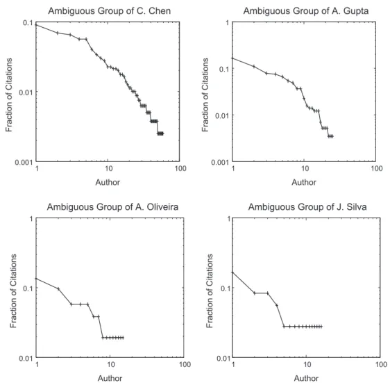
Table 3shows more detailed information about the collections and their ambiguous groups. Disambiguation is particu-larly difficult in ambiguous groups such as the ‘‘C. Chen’’ group, in which the correct author must be selected from 60 pos-sible authors, and in ambiguous groups such as the ‘‘J. Silva’’ group, in which the majority of authors appears in only one citation.Fig. 1shows the authorship distribution within each of two representative groups of each collection. Notice that, for a given group, few authors are very prolific and appear in several citations, while most of the authors appear in only few citations (the same trend is observed in all groups of DBLP and BDBComp). This is an intrinsic characteristic of scientific publications, as pointed out in (Liming & Lihua, 2005).

4.2. Evaluation Metrics

Disambiguation effectiveness, that is, the ability to properly select the author of a citation, is assessed through precision, recall and F1metrics. Precisionpis defined as the proportion of correctly disambiguated citations (i.e., citations for which the corresponding author was correctly predicted by the disambiguator). Recallris defined as the proportion of correctly dis-ambiguated citations out of all the citations having the target author. F1is defined as the harmonic mean of precision and recall (i.e.,2pr

pþr). Macro- and micro-averaging were applied to F1to get single effectiveness values. For F1macro-averaging (macroF1), scores were first computed for individual authors and then averaged over all authors. For F1micro-averaging (microF1), the decisions for all authors were counted in a joint pool. MacroF1and microF1are the primary metrics used in this paper.

4.3. Baselines

We used the two supervised name disambiguators proposed in (Han et al., 2004) as baselines. The first disambiguator uses the Naive Bayes probability model (Mitchell, 1997) and the second one uses Support Vector Machines (SVM) (Cortes & Vapnik, 1995). It is worth mentioning that, as described in the literature (Han et al., 2004), these disambiguators are rep-resentative supervised disambiguation methods for bibliographic citations that use the same set of features as us (coauthor names, work title and publication venue title) for the disambiguation task. For further details on these methods, please refer to (Han et al., 2004). We also employed the k-way spectral clustering (Han, Zha, et al., 2005) unsupervised disambiguator as baseline (in order to evaluate scenarios where no training example is available).

4.4. Results

All experiments were performed on a Linux-based PC with an Intel Core 2 Duo 1.83 GHz processor and 2GBytes RAM. All results presented were found to be statistically significant at the 95% confidence level when tested with the two-tailed

Table 3

The DBLP and BDBComp collections

DBLP BDBComp

Ambiguous group #Citations #Authors Ambiguous group #Citations #Authors

A. Gupta 576 26 A. Oliveira 52 16

A. Kumar 243 14 A. Silva 64 32

C. Chen 798 60 F. Silva 26 20

D. Johnson 368 15 J. Oliveira 48 18

J. Martin 112 16 J. Silva 36 17

J. Robinson 171 12 J. Souza 35 11

J. Smith 921 29 L. Silva 33 18

K. Tanaka 280 10 M. Silva 21 16

M. Brown 153 13 R. Santos 20 16

M. Jones 260 13 R. Silva 28 20

pairedt-test. For EAND, LAND and SLAND we set

r

min= 0.05. For SLAND, in particular, we investigated the sensitivity to

parameters

c

minandDmin. RBF kernels were used for SVM and we used a LibSVM tool (Chang & Lin, 2001) for finding their

optimum parameters for each ambiguous group. We used a non-parametric implementation for Naive Bayes (Domingos & Pazzani, 1997).

How effective are associative disambiguators compared with the baselines?

We evaluate the disambiguation effectiveness obtained by different disambiguators using DBLP and BDBComp collec-tions. Specifically, we performed 10-fold cross-validation within each ambiguous group, and the final result associated with each group represents the average of the ten runs.Table 4shows microF1and macroF1values for Naive Bayes, SVM, EAND and LAND in each ambiguous group.5_{In terms of microF}

1, EAND is in close rivalry with Naive Bayes and SVM, being a little better than Naive Bayes and little worse than SVM. LAND, on the other hand, shows an outstanding effectiveness, being the best performer in all ambiguous groups, with gains ranging from 1.8% (group of ‘‘K. Tanaka’’) to 15.2% (group of ‘‘J. Martin’’), and also on average (with gains of more than 6.3%, compared to Naive Bayes). Disambiguation effectiveness in terms of macroF1is also notorious. Again, EAND is very competitive with SVM and Naive Bayes, and LAND is the best performer in all ambiguous groups, with gains ranging from 2.5% (group of ‘‘K. Tanaka’’) to 23.4% (group of ‘‘D. Johnson’’). On average, gains range from 12.1% (com-pared to SVM) to 16.9% (com(com-pared to Naive Bayes). Even better results can be observed in the case of the BDBComp collection, as shown inTable 5. In this case, overall gains range from 32% (group of ‘‘A. Oliveira’’) to 466% (group of ‘‘F. Silva’’).

The main reason for this impressive disambiguation effectiveness is depicted inFig. 2. We selected some ambiguous groups, and for each group we sorted the corresponding authors in descending order of popularity (x-axis). Thus, more

0.001 0.01 0.1

1 10 100

Fraction of Citations

Author

Ambiguous Group of C. Chen

0.001 0.01 0.1 1

1 10 100

Fraction of Citations

Author

Ambiguous Group of A. Gupta

0.01 0.1 1

1 10 100

Fraction of Citations

Author

Ambiguous Group of A. Oliveira

0.01 0.1 1

1 10 100

Fraction of Citations

Author

Ambiguous Group of J. Silva

Fig. 1.Authorship distribution within each ambiguous group. Authors (x-axis) are sorted in decreasing order of prolificness (i.e., more prolific authors appear in the first positions).

prolific authors (i.e., authors appearing in more citations) appear first. They-axis shows microF1values associated with each author. In general, more prolific authors are better disambiguated. All disambiguators perform better, in general, when deal-ing with more popular/prolific authors. Disambiguation effectiveness tends to decrease with prolificness and this is mainly due to the reduction in the amount of examples available during training (i.e., there is only few citations associated with these authors). The crucial point is that, as shown inFig. 2, LAND is able to focus on producing functions that are suitable to disambiguate specific citations. This is because LAND builds the disambiguation function on a demand-driven basis, achieving higher effectiveness in less prolific authors, since important evidence supporting such authors are not discarded

Table 4

MicroF1and MacroF1values for the DBLP collection. Best results, including statistical ties, are highlighted in bold.

Ambiguous group NB SVM EAND LAND

A. Gupta 0.883 ± 0.036 0.874 ± 0.043 0.866 ± 0.040 0.921± 0.027

A. Kumar 0.837 ± 0.077 0.873 ± 0.077 0.899± 0.053 0.928± 0.059

C. Chen 0.794 ± 0.037 0.789 ± 0.039 0.793 ± 0.038 0.855± 0.037

D. Johnson 0.833 ± 0.078 0.876 ± 0.068 0.869 ± 0.050 0.911 ± 0.036

J. Martin 0.719 ± 0.105 0.748 ± 0.142 0.747 ± 0.141 0.827± 0.090

J. Robinson 0.861 ± 0.113 0.869 ± 0.083 0.825 ± 0.101 0.934 ± 0.069

J. Smith 0.873 ± 0.032 0.909 ± 0.033 0.873 ± 0.015 0.928 ± 0.028

K. Tanaka 0.917 ± 0.041 0.936 ± 0.053 0.928± 0.045 0.953 ± 0.054

M. Brown 0.878 ± 0.096 0.879 ± 0.085 0.886± 0.087 0.934 ± 0.064

M. Jones 0.855 ± 0.064 0.857 ± 0.051 0.844 ± 0.087 0.884 ± 0.052

M. Miller 0.935 ± 0.047 0.926 ± 0.026 0.931 ± 0.043 0.960 ± 0.032

Average 0.857 ± 0.023 0.870 ± 0.023 0.861 ± 0.012 0.911 ± 0.018

A. Gupta 0.763 ± 0.081 0.761 ± 0.0988 0.739 ± 0.079 0.866 ± 0.056

A. Kumar 0.715 ± 0.116 0.749 ± 0.142 0.810± 0.087 0.837 ± 0.097

C. Chen 0.654 ± 0.060 0.696 ± 0.061 0.682 ± 0.043 0.795 ± 0.061

D. Johnson 0.694 ± 0.099 0.790 ± 0.126 0.737 ± 0.100 0.856 ± 0.074

J. Martin 0.647 ± 0.115 0.646 ± 0.123 0.696± 0.145 0.758 ± 0.122

J. Robinson 0.822 ± 0.135 0.844 ± 0.092 0.782 ± 0.127 0.934 ± 0.068

J. Smith 0.672 ± 0.100 0.742 ± 0.077 0.685 ± 0.097 0.818 ± 0.102

K. Tanaka 0.835 ± 0.089 0.882 ± 0.105 0.848 ± 0.086 0.904 ± 0.111

M. Brown 0.843 ± 0.124 0.834 ± 0.143 0.858± 0.110 0.909 ± 0.106

M. Jones 0.721 ± 0.127 0.731 ± 0.118 0.719 ± 0.132 0.806 ± 0.104

M. Miller 0.735 ± 0.156 0.694 ± 0.117 0.733 ± 0.155 0.829 ± 0.134

Average 0.712 ± 0.037 0.743 ± 0.045 0.730 ± 0.027 0.833 ± 0.043

Table 5

MicroF1and MacroF1values for the BDBComp collection. Best results, including statistical ties, are highlighted in bold.

Ambiguous group NB SVM EAND LAND

A. Oliveira 0.497 ± 0.303 0.500 ± 0.327 0.515 ± 0.331 0.657 ± 0.236

A. Silva 0.283 ± 0.190 0.283 ± 0.190 0.258 ± 0.188 0.521 ± 0.172

F. Silva 0.050 ± 0.158 0.050 ± 0.158 0.083 ± 0.166 0.283 ± 0.352

J. Oliveira 0.450 ± 0.258 0.415 ± 0.208 0.412 ± 0.239 0.455 ± 0.259

J. Silva 0.400 ± 0.214 0.458 ± 0.249 0.428 ± 0.244 0.625 ± 0.267

J. Souza 0.617 ± 0.324 0.650 ± 0.266 0.622 ± 0.274 0.708 ± 0.201

L. Silva 0.217 ± 0.269 0.200 ± 0.243 0.230 ± 0.248 0.600 ± 0.251

M. Silva 0.000 ± 0.000 0.000 ± 0.000 0.000 ± 0.000 0.250 ± 0.264

R. Santos 0.000 ± 0.000 0.000 ± 0.000 0.000 ± 0.000 0.200 ± 0.350

R. Silva 0.117 ± 0.193 0.117 ± 0.193 0.107 ± 0.232 0.267 ± 0.251

Average 0.263 ± 0.113 0.267 ± 0.230 0.265 ± 0.238 0.457 ± 0.192

A. Oliveira 0.056 ± 0.042 0.125 ± 0.138 0.112 ± 0.094 0.172 ± 0.105

A. Silva 0.022 ± 0.021 0.033 ± 0.033 0.035 ± 0.029 0.089 ± 0.047

F. Silva 0.003 ± 0.010 0.025 ± 0.079 0.055 ± 0.053 0.105 ± 0.173

J. Oliveira 0.047 ± 0.025 0.085 ± 0.064 0.074 ± 0.022 0.112 ± 0.115

J. Silva 0.048 ± 0.028 0.133 ± 0.108 0.089 ± 0.058 0.195 ± 0.118

J. Souza 0.086 ± 0.056 0.177 ± 0.129 0.109 ± 0.071 0.240 ± 0.117

L. Silva 0.035 ± 0.031 0.021 ± 0.024 0.047 ± 0.031 0.136 ± 0.095

M. Silva 0.000 ± 0.000 0.000 ± 0.000 0.000 ± 0.000 0.063 ± 0.077

R. Santos 0.000 ± 0.000 0.000 ± 0.000 0.000 ± 0.000 0.055 ± 0.089

R. Silva 0.014 ± 0.022 0.042 ± 0.104 0.052 ± 0.089 0.068 ± 0.101

during rule extraction (i.e., multiple cut-off values are applied). Since less prolific authors, when considered together, corre-spond to a large number of citations, the ability of generating specific disambiguation functions according to a particular citation incurs in impressive gains in effectiveness.

0.6 0.65 0.7 0.75 0.8 0.85 0.9 0.95 1

5 10 15 20 25

MicroF1

Author

Ambiguous Group of A. Gupta

LAND EAND SVM Naive Bayes 0.6 0.65 0.7 0.75 0.8 0.85 0.9 0.95 1

1 2 3 4 5 6 7 8 9 10

MicroF1

Author

Ambiguous Group of A. Kumar

LAND EAND SVM Naive Bayes 0.6 0.65 0.7 0.75 0.8 0.85 0.9 0.95 1

10 20 30 40 50 60

MicroF1

Author

Ambiguous Group of C. Chen

LAND EAND SVM Naive Bayes 0.65 0.7 0.75 0.8 0.85 0.9 0.95 1

1 2 3 4 5 6 7 8 9 10

MicroF1

Author

Ambiguous Group of M. Jones

LAND EAND SVM Naive Bayes 0.55 0.6 0.65 0.7 0.75 0.8 0.85 0.9 0.95 1

5 10 15 20 25

MicroF1

Author

Ambiguous Group of J. Smith

LAND EAND SVM Naive Bayes 0.65 0.7 0.75 0.8 0.85 0.9 0.95 1

2 4 6 8 10 12

MicroF1

Author

Ambiguous Group of J. Martin

LAND EAND SVM Naive Bayes

How the different disambiguators perform with limited labeling efforts?

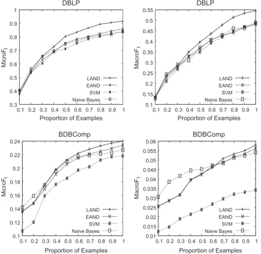
We evaluate the disambiguation effectiveness obtained by each disambiguator by varying the fraction of available exam-ples. None of the disambiguators evaluated in this experiment exploit unlabeled data (which, in this case, correspond to cita-tions in the test set) to increase the number of available examples (note that LAND simply uses citacita-tions in the test set to guide the lazy search for useful rules, but not as additional training examples). For this experiment, we performed 5-fold cross-validation within each ambiguous group and, from the original training data associated with each fold, we produce 10 subsets, where each subset contains a different fraction of examples which were randomly selected from the training data (i.e., 10%, 20%,. . ., 100% of the citations in the training data associated with each fold). In the results, which are depicted in Fig. 3, each point represents the average of the five runs, which are then averaged over all ambiguous groups (i.e., similar to the last line ofTable 4).

For both collections, the effectiveness of all disambiguators are very similar when only few examples are available. How-ever, when more examples are available, LAND achieves superior effectiveness compared to the baselines. In such cases, for the DBLP collection, LAND showed a significant improvement (both in terms of microF1and macroF1). On the other hand, for the BDBComp collection, the effectiveness of Naive Bayes, EAND and LAND are very close. While high effectiveness was ob-served in the DBLP collection, a very low effectiveness (specially in terms of macroF1) was obtained in the BDBComp collec-tion. This is because the BDBComp collection contains many authors that appear only in the test set (most of them appearing in only one citation) and, thus, the predictions for the citations being authored by these authors are always wrong (since there is no example supporting these authors in the training data). Next, we will evaluate SLAND, which has the ability to detect unseen authors (i.e., authors appearing only on citations in the test set) and to enhance the training data by incor-porating additional examples.

How does

c

minimpact the effectiveness of SLAND?

We evaluate the effectiveness of SLAND in detecting unseen authors using the BDBComp collection. Differently from the DBLP collection, the BDBComp collection contains many unseen authors. Specifically, 43.5% of the authors appear only in the test set. For this experiment, we, again, perform 5-fold cross-validation, following the same strategy used in the previous experiment. However, for each fraction of training examples, we varied

c

minfrom 1 to 6. The results are shown inFig. 4.

0.3 0.4 0.5 0.6 0.7 0.8 0.9 1

0.1 0.2 0.3 0.4 0.5 0.6 0.7 0.8 0.9 1

MicroF

1

Proportion of Examples

DBLP

LAND EAND SVM Naive Bayes 0.1 0.15 0.2 0.25 0.3 0.35 0.4 0.45 0.5 0.55

0.1 0.2 0.3 0.4 0.5 0.6 0.7 0.8 0.9 1

MacroF

1

Proportion of Examples

DBLP

LAND EAND SVM Naive Bayes 0.1 0.12 0.14 0.16 0.18 0.2 0.22 0.24

0.1 0.2 0.3 0.4 0.5 0.6 0.7 0.8 0.9 1

MicroF

1

Proportion of Examples

BDBComp

LAND EAND SVM Naive Bayes 0.01 0.015 0.02 0.025 0.03 0.035 0.04 0.045 0.05 0.055 0.06

0.1 0.2 0.3 0.4 0.5 0.6 0.7 0.8 0.9 1

MacroF

1

Proportion of Examples

BDBComp

LAND EAND SVM Naive Bayes

For the BDBComp collection, the fraction of unseen authors that are detected (number of detected unseen authors divided by total number of unseen authors) increases with

c

min. This is expected, since the amount of evidence that is required to

rec-ognize an author as already seen, increases for higher values of

c

min. Further, it becomes more difficult to detect an unseen

author when the fraction of training examples increases. This is because, in such cases, (1) more authors are seen (i.e., there are more examples), and (2) there is an increase in the amount of available evidence supporting already seen authors.

How doesDminimpact the effectiveness of SLAND?

We evaluate the effectiveness of SLAND in incorporating new training examples using the DBLP collection, since this col-lection contains much more citations in the test set. Again, we perform 5-fold cross-validation, following the same strategy used in the previous experiment. However, for each fraction of training examples, we variedDminfrom 0.5 to 0.9. The results

are shown inFig. 5. As it can be seen, the effectiveness of SLAND decreases whenDmin(i.e., the minimum reliability required

to consider a prediction as reliable) is set too high (i.e.,Dmin> 0.75). Further, the effectiveness also decreases whenDminis set

too low (i.e.,Dmin< 0.65). On one hand, when lower values ofDminare applied, several citations in the test set, which are

associated with wrong predictions, are included in the training data (note that the reliability of a prediction decreases with Dmin), hurting effectiveness. On the other hand, when higher values ofDminare applied, only few citations in the test set are

included in the training data. For the DBLP collection, SLAND achieves the best effectiveness whenDminis between 0.65 and

0.75 (specially when few training examples are available).

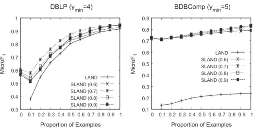
How effective is SLAND compared with LAND?

We now evaluate how the abilities of SLAND improve its effectiveness when compared to LAND. We, again, perform 5-fold cross-validation, following the same strategy used in the previous experiments.Fig. 6shows some of the results. The value associated with each point in each graph is obtained by applying a different combination of

c

minandDmin, for different

fractions of training examples. For the DBLP collection, gains ranging from 18.4% to 53.8% are observed when few training examples are available. The improvement decreases when more examples are available, since in this case (1) more authors are seen and (2) additional examples that are included in the training data do not impact so much the final effectiveness. Interestingly, SLAND achieves good effectiveness even when not a single example is available for training. This is possible because, in this case, citations authored by unseen authors are included in the training data, and used as training examples. These gains highlight the advantages of self-training.

Improvements obtained using the BDBComp collection are more impressive. As discussed before, this collection contains several authors that appear in only one citation. LAND (and other completely supervised methods) is not useful in such sce-narios, since it is not able to produce correct disambiguation functions for such citations (i.e., if this citation appears only in the test set, then the training data contains no evidence supporting the correct author). SLAND, on the other hand, is highly effective in such cases, being able to detect unseen authors, and to make use of this information to enhance the training data with additional examples. As a result, improvements provided by SLAND range from 241.6% to 407.1%. Thus, SLAND is not only able to reduce labeling efforts (as shown in the experiments with the DBLP collection), but it is also able to detect novel and important information (i.e., unseen authors), being highly practical and effective in a variety of scenarios.

How effective is SLAND compared to an unsupervised disambiguator?

We used the DBLP collection to perform a comparison between SLAND (

c

min= 4,Dmin= 0.7), and the k-way spectral

clus-tering disambiguator (Han, Zha, et al., 2005), when no training example is available for any of the disambiguators. We adopted the evaluation methodology proposed in (Han, Zha, et al., 2005), so that we can directly compare the effectiveness of both disambiguators. In this case, a confusion matrix is used to assess the microF1. A different confusion matrix is asso-ciated with each ambiguous group, and the final effectiveness is represented by the accuracy averaged over all groups.

0.55 0.6 0.65 0.7 0.75 0.8 0.85

1 2 3 4 5 6

Fraction of Unseen Authors Detected

y_min

BDBComp

0.1 0.2 0.3 0.4 0.5 0.6 0.7

Both disambiguators are statistically tied on almost all ambiguous groups (seeTable 6). The K-way spectral clustering disambiguator obtained superior effectiveness on three ambiguous groups, while SLAND was superior in one ambiguous group. It is important to notice that the k-way spectral clustering disambiguator takes as input the correct number of clusters to be generated, that is, if there aremauthors in a group, then this group is clustered into exactlymclusters (Han, Zha, et al., 2005). This is clearly unrealistic in an actual or practical scenario, but provides something closer to an upper-bound for an

0.45 0.5 0.55 0.6 0.65 0.7 0.75 0.8 0.85 0.9 0.95 0.1 0.2 0.3 0.4 0.5 0.6 0.7 0.8 0.9 1 Proportion of Examples 0.5

0.6 0.7 0.8 0.9 Minimum Reliability 0.4 0.5 0.6 0.7 0.8 0.9 1 MicroF₁

Fig. 5.Sensitivity toDmin.

0.3 0.4 0.5 0.6 0.7 0.8 0.9 1

0 0.1 0.2 0.3 0.4 0.5 0.6 0.7 0.8 0.9 1

MicroF

1

Proportion of Examples

DBLP (y

_min

=4)

LAND SLAND (0.6) SLAND (0.7) SLAND (0.8) SLAND (0.9) 0.1 0.2 0.3 0.4 0.5 0.6 0.7 0.8 0.9

0 0.1 0.2 0.3 0.4 0.5 0.6 0.7 0.8 0.9 1

MicroF

1

Proportion of Examples

BDBComp (y

_min

=5)

LAND SLAND (0.6) SLAND (0.7) SLAND (0.8) SLAND (0.9)

Fig. 6.MicroF1values for differentDminandcmin(Dminvalues are between parentheses).

Table 6

SLAND compared to the K-way spectral clustering disambiguator in terms of microF1on the DBLP collection. Best results, including statistical ties, are highlighted in bold.

Ambiguous group MicroF1

SLAND K-Way SC

A. Gupta 0.453 ± 0.050 0.546 ± 0.048

A. Kumar 0.555 ± 0.150 0.505 ± 0.029

C. Chen 0.365 ± 0.052 0.607 ± 0.050

D. Johnson 0.710 ± 0.062 0.561 ± 0.081

J. Martin 0.786 ± 0.058 0.939 ± 0.062

J. Robinson 0.662 ± 0.103 0.693 ± 0.051

J. Smith 0.444 ± 0.057 0.500 ± 0.097

K. Tanaka 0.554 ± 0.099 0.626 ± 0.120

M. Brown 0.680 ± 0.133 0.759 ± 0.143

M. Jones 0.504 ± 0.179 0.628 ± 0.083

M. Miller 0.699 ± 0.126 0.479 ± 0.117

unsupervised disambiguator that has privileged information. SLAND, on the other hand, does not use this information, and works by detecting unseen authors, and incrementally adding new examples to the training data. Other point worth men-tioning is that, as shown inFig. 6, with small labeling efforts, the effectiveness of SLAND can be much improved (greatly out-perfoming the unsupervised disambiguator), demonstrating that SLAND is very cost-effective.

5. Conclusions and future work

Name disambiguation, in the context of bibliographic citations, is the problem of determining whether records in a col-lection of publications refer to the same person. This problem is widespread in many large-scale digital libraries, such as Citeseer, Google Scholar and DBLP.

Authorship frequency follows a very skewed distribution. Few authors are very prolific while most of the authors are in-cluded in only few citations. This property seems to affect the effectiveness of disambiguators based on machine learning techniques such as Naive Bayes and SVM. Thus, in this article we propose a novel approach for name disambiguation that uncovers associations between bibliographic features and authors. The proposed disambiguators based on this approach were evaluated showing competitive results. LAND, in particular, which is based on a demand-driven rule generation pro-cess, showed superior effectiveness when compared to the state-of-the-art. A deep analysis revealed that the outstanding effectiveness of LAND is mainly because it builds disambiguation functions on a demand-driven basis, so that authors appearing in only few citations can be better disambiguated. Other factors that greatly affect disambiguation effectiveness include the prohibitive cost of labeling vast amounts of examples and the appearance of unseen authors. Thus, we extend LAND with the self-training ability. The resulting disambiguator, SLAND, drastically reduces the amount of examples re-quired to build effective disambiguation functions, and is also competent in detecting unseen authors. The self-training abil-ity makes SLAND highly effective and practical. In fact, we already have initial evidence that SLAND can be very effective even in situations in which the training data is automatically produced, i.e., with no manual labeling at all (Ferreira, Veloso, Gonçalves, & Laender, 2010).

As future work, we intend to perform experiments with other collections, particularly from fields other than Computer Science, as well as considering other features like those extracted from headers of scientific papers (e.g., affiliation, address, e-mail), obtained from collaborative social networks, or from the topics or categories of the citations.

Acknowledgments

This research is partially funded by the National Institute of Science and Technology for the Web (InWeb) (MCT/CNPq/ FAPEMIG Grant No. 573871/2008-6), and by the authors’s individual research Grants from CAPES, CNPq, and FAPEMIG.

References

Agrawal, R., Imielinski, T., & Swami, A. (1993). Mining association rules between sets of items in large databases. InProceedings of the 1993 ACM SIGMOD international conference on management of data(pp. 207–216). Washington, USA.

Bekkerman, R., & McCallum, A. (2005). Disambiguating web appearances of people in a social network. InProceedings of the 14th international conference on world wide web(pp. 463–470). Chiba, Japan.

Bhattacharya, I., & Getoor, L. (2006). A latent dirichlet model for unsupervised entity resolution. InProceedings of the Sixth SIAM international conference on data mining. Bethesda, MD, USA.

Bhattacharya, I., & Getoor, L. (2007). Collective entity resolution in relational data.ACM Transactions on Knowledge Discovery from Data, 1. Chang, C. -C., & Lin, C. -J. (2001).LibSVM: A library for support vector machines. Software available at <http://www.csie.ntu.edu.tw/cjlin/libsvm>. Cortes, C., & Vapnik, V. (1995). Support-vector networks.Machine Learning, 20, 273–297.

Cota, R. G., Ferreira, A. A., Nascimento, C., Gonçalves, M. A., & Laender, A. H. F. (2010). An unsupervised heuristic-based hierarchical method for name disambiguation in bibliographic citations.JASIST, 61, 1853–1870.

Cota, R. G., Gonçalves, M. A., & Laender, A. H. F. (2007). A heuristic-based hierarchical clustering method for author name disambiguation in digital libraries. InProceedings of the XXII Brazilian symposium on databases(pp. 20–34). João Pessoa, Paraiba, Brazil.

Culotta, A., Kanani, P., Hall, R., Wick, M., & McCallum, A. (2007). Author disambiguation using error-driven machine learning with a ranking loss function. In International workshop on information integration on the web. Vancouver, Canada.

Dhillon, I. S., Guan, Y., & Kulis, B. (2005). A fast kernel-based multilevel algorithm for graph clustering. InProceedings of the 11th ACM SIGKDD international conference on knowledge discovery and data mining(pp. 629–634). Chicago, Illinois, USA.

Domingos, P., & Pazzani, M. (1997). On the optimality of the simple Bayesian classifier under zero-one loss.Machine Learning, 29, 103–137.

Ester, M., Kriegel, H. -P., Sander, J., & Xu, X. (1996). A density-based algorithm for discovering clusters in large spatial databases with noise. InProceedings of the 2nd international conference on knowledge discovery and data mining(pp. 226–231). Portland, Oregon.

Ferreira, A. A., Veloso, A., Gonçalves, M. A., & Laender, A. H. F. (2010). Effective self-training author name disambiguation in scholarly digital libraries. In Proceedings of the 2010 ACM/IEEE joint conference on digital libraries(pp. 39–48). Gold Coast, Queensland, Australia.

Goethals, B., & Zaki, M. (2004). Advances in frequent itemset mining implementations: report on FIMI’03.SIGKDD Explorations, 6, 109–117.

Han, H., Giles, C. L., Zha, H., Li, C., & Tsioutsiouliklis, K. (2004). Two supervised learning approaches for name disambiguation in author citations. In Proceedings of the 4th ACM/IEEE-CS joint conference on digital libraries(pp. 296–305). Tuscon, USA.

Han, H., Xu, W., Zha, H., & Giles, C. L. (2005). A hierarchical naive Bayes mixture model for name disambiguation in author citations. InProceedings of the 2005 ACM symposium on applied computing(pp. 1065–1069). Santa Fe, New Mexico, USA.

Han, H., Zha, H., & Giles, C. L. (2005). Name disambiguation in author citations using a k-way spectral clustering method. InProceedings of the 5th ACM/IEEE joint conference on digital libraries(pp. 334–343). Denver, CO, USA.

Huang, J., Ertekin, S., & Giles, C. L. (2006). Efficient name disambiguation for large-scale databases. InProceedings of the 10th European conference on principles and practice of knowledge discovery in databases(pp. 536–544). Berlin, Germany.