SOIL EROSION FRAGILITY ASSESSMENT USING
AN IMPACT MODEL AND GEOGRAPHIC
INFORMATION SYSTEM
Luiz Alberto Blanco Jorge
UNESP/FCA - Depto. Recursos Naturais - C.P. 237 - 18603-970 - Botucatu, SP - Brasil - e-mail <blanco@fca.unesp.br>
ABSTRACT: A study was taken in a 1566 ha watershed situated in the Capivara River basin, municipality of Botucatu, São Paulo State, Brazil. This environment is fragile and can be subjected to different forms of negative impacts, among them soil erosion by water. The main objective of the research was to develop a methodology for the assessment of soil erosion fragility at the various different watershed positions, using the geographic information system ILWIS version 3.3 for Windows. An impact model was created to generate the soil’s erosion fragility plan, based on four indicators of fragility to water erosion: land use and cover, slope, percentage of soil fine sand and accumulated water flow. Thematic plans were generated in a geographic information system (GIS) environment. First, all the variables, except land use and cover, were described by continuous numerical plans in a raster structure.The land use and cover plan was also represented by numerical values associated with the weights attributed to each class, starting from a pairwise comparison matrix and using the analytical hierarchy process. A final field check was done to record evidence of erosive processes in the areas indicated as presenting the highest levels of fragility, i.e., sites with steep slopes, high percentage of soil fine sand, tendency to accumulate surface water flow, and sites of pastureland. The methodology used in the environmental problems diagnosis of the study area can be employed at places with similar relief, soil and climatic conditions.
Key words: water flow, hydric erosion, analytical hierarchy process
AVALIAÇÃO DA FRAGILIDADE À EROSÃO DO SOLO POR MEIO
DE UM MODELO DE IMPACTO E SISTEMA DE
INFORMAÇÕES GEOGRÁFICAS
RESUMO:A área de estudo, com 1566 ha, abrange uma microbacia hidrográfica, posicionada em local de relevo em contato reverso-frente de cuesta-depressão periférica paulista, inclusa na Bacia do Rio Capivara, no município de Botucatu, Estado de São Paulo. Esse ambiente é frágil, podendo sofrer diferentes formas de impactos negativos, dentre as quais a erosão hídrica do solo. O objetivo principal foi desenvolver uma metodologia, com auxílio do sistema de informações geográficas ILWIS v. 3.3 para Windows, para avaliar a fragilidade à erosão do solo em diferentes posições na microbacia. Um modelo de impacto foi criado para gerar o plano de fragilidade à erosão do solo, com base em quatro planos temáticos relacionados com indicadores de fragilidade a erosão hídrica: uso e cobertura do solo, declividade, percentagem de areia fina e acúmulo de fluxo de água. Em um primeiro passo, excetuando-se o uso e cobertura do solo, as outras três variáveis foram descritas por planos numéricos contínuos em estrutura raster. O plano de uso e cobertura do solo pôde ser representado também por valores numéricos, associados a pesos atribuídos a cada classe, a partir de uma matriz de comparação por pares, considerando-se o método de hierarquia analítica. Realizou-se uma checagem de campo final, em que foram registradas evidências de processos erosivos, naquelas áreas apontadas como apresentando maiores níveis de fragilidade, ou seja, locais com declividade acentuada, solo com alta percentagem de areia fina, tendência de acúmulo de fluxo superficial de água e ocupadas por pastagem. A metodologia desenvolvida pode ser usada no diagnóstico de problemas ambientais em locais com condições similares às da área de estudo.
Palavras-chave: fluxo de água, erosão hídrica, método de hierarquia analítica
INTRODUCTION
Among the descriptive and interpretive aspects of
threats, and an estimate of the fragility or vulnerabil-ity for the development of human activities.
Water erosion assessment, which is part of the di-agnosis of environmental problems, is highly relevant since inadequate land use can accelerate the processes of erosion and deposition that occur naturally, leading to modifications related to soil conservation, water production and quality, and environmental changes in certain locations of a drainage basin. Various ap-proaches and equations for risk assessment or predic-tive evaluation of soil erosion by water are available in literature. Among then the universal soil loss equation (Wischmeier & Smith, 1965, 1978) and the revised universal soil loss equation (Renard et al., 1994; Yoder & Lown, 1995). Wu & Wang (2007) proposed a model to evaluate the risk index for soil erosion by water, in which the remote sensing, GIS, the analyti-cal hierarchy process (AHP) and modeling techniques are integrated.
The present study was undertaken in a 1,566 ha watershed situated in a cuesta relief area of São Paulo State Peripheral Depression. This environment is ex-tremely fragile and can be subjected to different forms of negative impacts, including soil erosion. The main objective was to develop a methodology, aided by the geographic information system ILWIS version 3.3 for Windows, to assess the soil’s fragility to erosion by water at the different sites.
MATERIAL AND METHODS
Study area
The watershed is located in the Capivara River ba-sin in the municipality of Botucatu, São Paulo State, Brazil (Figure 1). It comprises: i – a small area at the cuesta reverse (beginning of the S. Paulo Eastern Pla-teau), with altitudes of 700 to 810 m; ii – a cuesta front (a sandstone and basaltic escarpment with their origi-nated soils ); and iii – a peripheral depression segment, with altitudes from 465 to 600 m, comprising an area of sandstones and alluvial sediments encompassing the Capivara River wetlands. The soils of the Capivara River flat wetlands are Dystric Fluvisols, Mollic Gleysols and Dystric Gleysols. Toward the front of the cuesta, but still within the peripheral depression there are frequent gently undulating uprisings (2 to 20% slope) with Albic Arenosols, Acric Ferralsols, Rhodic Ferralsols, Chromic Luvisols, Dystric Nitisols and Haplic Chernozems. The basaltic cuesta front have Lithosols on 20% to 40% slopes. Rock’s outcrops are frequent on scarped relief areas, where slopes exceed 40% (Carvalho et al., 1991).
The climate has two distinct seasons, one rainy and hot (September to March) and the other dry and cold (April to August). The native vegetation partially loses its leaves in the dry cold season. It is classified as Semidecidual Seasonal Forest (Veloso, 1992), with
fragments of altered forest that have undergone vari-ous levels of anthropic disturbance. Fragments of natu-ral vegetation, a transition of forest to forested savanna (cerradão) and gallery forest, are also present. Land is used mainly as pasture. Small areas are planted with forests and cultivated as farmland.
Digital elevation model and slope
A digital elevation model (DEM) is defined as a nu-merical structure of data that represents the spatial dis-tribution of the altitude of the terrain’s surface (Felicísimo, 1994). The DEMs were integrated to the GIS, offering a series of applications and different op-tions of usage. One of these opop-tions is the generation of new spatial data based on DEMs, such as slope, aspect, effects of illumination, determination of the water route, etc.
The study area database was structured (from 2005 to 2007) in the geographic information system ILWIS for Windows (International Institute for Geo-Informa-tion Science and Earth ObservaGeo-Informa-tion, 2001) environ-ment. The two study area planialtimetric maps were digitized (using a scanner) and georeferenced. The maps were used as the basis for the spatial data input operation. The watershed’s boundaries, the contour lines, the summit elevations, and the drainage network were digitized. After digitizing the contour lines, the digital elevation model of the watershed and the the-matic slope plan were created in the GIS environment.
Orthophotos and land use plan
Orthophotos were generated based on aerial pho-tographs taken in the 2000 and 2005 years. These orthophotos served as the basis for outlining the land use and cover plan. The procedure to produce the orthophotos can be subdivided into the following steps: (i) acquisition of the aerial photography in digital form; (ii) creation of a georeference; (iii) specification of the system of coordinates and of the file of the digital el-evation model utilized; (iv) recording of the fiducial markers, which consists of the specification of the fo-cal distance of the camera and of the photo coordi-nates of the fiducial markers; (v) indication of the con-trol points detected in the aerial photography and on a map (Secretaria de Economia e Planejamento do Estado de São Paulo, scale 1:10000, UTM projection).
Water flow direction and flow accumulation
The planes of water flow direction and flow ac-cumulation were generated in the ILWIS environment, based on the digital elevation model (DEM). The lat-ter plan is related to the concept of contribution area. Any watershed may contain a large variety of geologi-cal, topographigeologi-cal, soil, vegetation and land use fea-tures that will affect the relation between precipitation
and flow. There are many points, which show a simi-lar hydrologic behavior, with simisimi-lar water balance and runoff characteristics. The hydrologic similarity index was developed as part of the rainfall-runoff model named the Topmodel (Beven, 2001). One of the basic premises of Topmodel has to do with the dynamics of saturated regions of the watershed that can be ap-proximated considering successive representations of the saturated zone of an area “a” drained to a point of the slope (contribution area).
Soil attribute
Soil sampling points were defined starting from a regular grid allocated so that the interval between points in the X and Y directions was 500 m, using the navigation capacity of the GPS to reach each point. Sixty-three points were sampled. At each point, a sample was taken at the 0 to 20 cm soil depth. The soil samples were analyzed to obtain information about the granulometry, with emphasis on the percentage of fine sand.
Attributing the soil sampling points to their respec-tive plan coordinates obtained by GPS, a connection was drawn between the location of these points and the variable of the soil, whose results were tabulated into a table of attributes. The spatial correlation mod-ule of ILWIS provided experimental semivariogram about the spatial behavior of the variable of the soil property. A semivariogram is a variance graph of paired sample measures. It provides a means to quantify the commonly grouped samples observed tendency to have more approximate values than more widely separated samples. The semivariogram described by Isaaks & Srivastava (1989), which provides the spatial depen-dence, is expressed by:
[
]
21
) ( ) ( 2
1 )
(
∑
=
+ −
= N
i
i
i Z x h
x Z N h
γ
where: γ(h) = semivariance for the distance h; xi and xi + h = sampling sites separated by the distance h; Z(xi) and Z(xi + h) = measured values of the variable.
spa-tial autocorrelation, the spaspa-tial distribution pattern is considered random. The interpretation of the two sta-tistics can be summarized as: 0 < C < 1 and I > 0 strong positive autocorrelation; C > 1 and I < 0 strong negative autocorrelation; C = 1 and I = 0 random dis-tributions of the values.
The power, exponential and Gaussian models were tested to adjust the estimated semivariogram in the GIS environment. The appropriate model was selected to describe the semivariance of the variable as a func-tion of the coefficient of determinafunc-tion (R2), of the
sum of squares of residues (SSR) and of the mean percentage deviations (MPD). Entering the estimators of the selected model into the ILWIS kriging mod-ule, using the ordinary kriging method, the values ob-tained at the sampled points were interpolated, deriving the corresponding continuous plan in a raster struc-ture.
Soil erosion fragility
The soil erosion fragility layer was drawn from the four thematic plans generated in the geographic infor-mation system environment: land use and cover, slope, percentage of fine sand, and water flow accumulation. The landscape elements were chosen as indicators of soil erosion fragility based on the field survey and in-formation analysis, combined with professional expert judgment. In the first step, all the variables except land use and cover were described by continuous numeri-cal plans in a raster structure.
The land use and cover plan was also represented as numerical values associated to weights attributed to each class, based on a pairwise comparison matrix, considering the analytical hierarchy process-AHP. The significances of land use and cover classes for fragil-ity to soil erosion by water were compared mutually and dissimilarities between their levels of importance were quantified, by the numbers 1 to 9, to indicate es-calated differences, while reciprocals of those num-bers were specified to their comparisons with an in-verse order. Specifically, number 1 means that levels of importance for both classes are equal while num-ber 9 represents that the level of importance for the first one is extremely higher than for the second one, according to the methodology presented by Saaty (1977). Using the AHP, the consistency of the alloca-tion of weights to the classes of criteria involved was evaluated. The latent root and the consistency index (CI) (CI = latent root – n) / (n – 1); n = number of lines / columns in the comparison matrix) were cal-culated. One then obtains the consistency ratio (CR) by dividing the consistency index by the random in-dex (RI), which has a fixed value (Bantayan & Bishop, 1998).
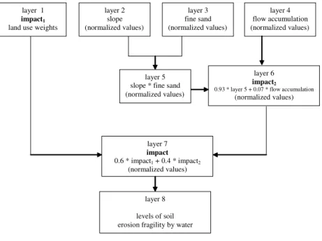
An impact model, considering the first impact layer (land use weights) and the second impact layer (w21 * (slope * fine sand) + w22 * flow accumulation), was proposed to generate the erosion fragility map:
fragility = w1 . impact1 + w2 . impact2
where: fragility = soil erosion fragility layer; impact1 = first impact layer; impact2 = second impact layer; w1, w2, w21, w22 = assigned weights.
The highest values obtained after the layer was nor-malized indicate points of greater fragility, i.e., points where the land cover has a smaller protection capac-ity and the impact is greater (areas of higher slope grade and percentage of fine sand, greater concentra-tion of water flow during rainfall). The layer was clas-sified into five levels of fragility.
The Cohen’s kappa coefficient, used as a measure of model accuracy and validation, was derived from the cross-tabulation of the mapped levels of soil ero-sion fragility against those observed in the 60 ground control points. The kappa statistic is expressed by:
kappa =
) 1 ( e
e o
P P P
− −
where: Po = observed agreement; Pe = expected agree-ment;
Kappa is a measure of the difference, standardized to lie on a –1 to 1 scale, where 1 is perfect agree-ment, 0 is exactly what would be expected by chance, and negative values indicate agreement less than chance. Interpretation of the statistic according to Landis & Koch (1977) is shown in Table 1.
RESULTS AND DISCUSSION
The sites with the highest slope values of the wa-tershed are located at the cuesta front (Figure 2). Sev-enteen land use and cover categories (Table 2) were observed in the study area. The values (weights) at-tributed to the different classes of land use and cover can be considered satisfactory, since the calculated consistency ratio (CR) is lower than 0.10 (Table 3, underneath). The highest weights correspond to the land use classes that offer the least protection against soil erosion by water (Table 3 and Figure 3).
Figure 2 - Slope classes map of the study area.
Entering the percentage of fine sand values (Fig-ure 5) into the ILWIS spatial correlation module re-sulted in the experimental semivariogram from the spa-tial behavior of the variables. The theoretical semivariogram was also adjusted (Table 4). The semivariogram of the variable percentage of fine sand did not show stabilization of the semivariance, con-sidering the maximum distances between pairs of sampled points. The power model adjusted adequately to experimental values, which can be ascertained by analyzing the coefficient of determination - R2, the sum
of squares of residues - SSR and the mean percent-age deviations - MPD (Table 4).
In addition to the Table 5 data the values of the statistics I of Moran (1948) and Geary’s C (1954) were obtained, which allow one to evaluate the ex-istence of autocorrelation or random distribution of the variable. An analysis of the values of I and C (Table 5) reveals that the variable percent of fine
Table 2 - The occupied surfaces and proportions of the different land uses and covers existing in the area.
r e v o c d n a e s u d n a
L area(ha) %
) A B ( o o b m a
B 1.05 0.07
) F C ( d n a l m r a f d e t a v i t l u
C 105.28 6.72
) P E ( s s e c o r p e v i s o r
E 5.76 0.37
) R F ( t n e m i r e p x e n o i t a r o t s e r t s e r o
F 9.77 0.62
) R T ( s e e r t f o p u o r
G 0.24 0.02
) R O ( d r a h c r
O 7.89 0.50
) L P ( d n a l e r u t s a
P 415.86 26.56
) F P ( t s e r o f d e t n a l
P 52.61 3.36
) R Q ( y r r a u
Q 3.43 0.22
) P R ( t c e j o r p n o i t a g i r r i e c i
R 38.91 2.48
) W R ( d n a l d o o w n a i r a p i
R 26.13 1.67
) D R ( d a o
R 2.40 0.15
) M I ( t n e m e v o r p m i a e r a l a r u
R 1.11 0.07
) B R ( g n i d l i u b l a r u
R 1.01 0.06
) F S ( t s e r o f l a n o s a e s l a u d i c e d i m e
S 668.26 42.68
) S F ( n o i t i s n a r t a n n a v a s d e t s e r o f o t t s e r o
F 165.26 10.55
) L W ( d n a l t e
W 61.03 3.90
l a t o
T 1566.00 100.00
Table 1 - Interpretation of kappa.
a p p a
K Agreement
0 0 . 0
< Less thanchance agreement
0 2 . 0 -1 0 .
0 Slightagreement
0 4 . 0 -1 2 .
0 Fair agreement
0 6 . 0 -1 4 .
0 Moderate agreement
0 8 . 0 -1 6 .
0 Substantialagreement
9 9 . 0 -1 8 .
0 Almostperfectagreement
Figure 3 - Weights attributed to land use and cover classes.
Figure 4 - Classes of water flow accumulation normalized values.
Figure 6 - Semivariogram – percentage of soil fine sand at the 0 to 20 cm depth.
200 300 400 500 600 700 800 900
500 1000 1500 2000 2500 3000 3500 4000 4500
Se
m
iv
a
ri
a
n
c
e
Distance (m)
% Fine Sand (0 - 20 cm)
Experimental Semivariance Power model
After adjustment of the estimated semivariogram by entering the coefficients of the model into the GIS kriging model, the continuous plan was derived for the variable percentage of fine sand in the 0 to 20 cm depth (Figure 6 and 7).
The four thematic plans related to water erosion fragility landscape elements were used to produce the erosion fragility map, according to the proposed mod-eling approach (Figure 8). The weights were assigned in the model after the field surveys. The impact layer was classified into five levels of fragility (Figure 9). The kappa coefficient value of 0.61 indicated a sub-stantial agreement between the model and the ground control points.
Fragility levels 3, 4 and 5 allow one to detect the areas in the landscape where the phenomenon of ero-sion is the most intense. In the final check after gen-erating the soil erosion fragility map, the main ero-sive processes occurring in the watershed under study were recorded using photographs taken at each site. The photographs (Figure 9) is a sample of the comparison between the highest levels of fragility shown in the thematic plan and the reality found in the field.
Photograph 1 (Figure 9) depicts a linear erosive process (fragility levels 3 and 4) found within a forest fragment that regenerated from a pastureland. Photograph 2 shows gully erosion in an area (level 3 of fragility in the surroundings and levels 4 and 5 at the sites of the erosive process) situated at the head of a drainage channel, in an area of pasture with steep slope and a soil with high percentage of fine sand. Photograph 3 depicts a situation (level 3 of fragility) occurring at a site
that encompasses the three aforementioned land-scape elements: the land use is pasture, the slope is steep, and there is a high percentage of fine sand. The methodology employed to evaluate the erosion fragility can be used for the detection of processes that have already occurred and/or are evolving, but it also seeks to identify areas with a potential for soil loss.
CONCLUSIONS
The final check, performed in the field to record evidence of erosive processes, indicated a good agreement with the levels of fragility to water ero-sion as calculated for the thematic plan. Therefore, the methodology used in the environmental prob-lems’ diagnosis of the study area can be employed at places with similar relief, soil and climatic con-ditions.
e l b a i r a
V Depth(cm) Model Nuggeteffect slope power R2 SSR MPD(%)
d n a s e n i f f o
% 0- 20 power 250.00 0.11500 1.000 0.9716 5932.1118 4.06
Table 4 - Semivariogram estimators of soil attribute.
Figure 7 - Percentage of soil fine sand layer (0 to 20 cm of depth).
) m ( e c n a t s i
d nr pairs I C Experimentalsemivariance Fittedsemivariance
0 0
5 188 0.248 0.63 303.08 307.50
0 0 0
1 260 0.109 0.80 386.48 365.00
0 0 5
1 297 0.048 0.88 423.97 422.50
0 0 0
2 395 0.020 0.89 432.39 480.00
0 0 5
2 291 -0.125 1.13 548.47 537.50
0 0 0
3 251 -0.133 1.17 568.35 595.00
0 0 5
3 165 -0.204 1.42 688.44 652.50
0 0 0
4 79 -0.184 1.41 683.51 710.00
0 0 5
4 25 -0.366 1.62 786.43 767.50
Table 5 - Results of the experimental semivariances and the semivariances estimated by the power model adjusted to the data of percentage of fine sand at the depth of 0 to 20 cm.
I = Moran’s spatial autocorrelation coefficient; C = Geary’s spatial autocorrelation coefficient. latent root: 9.00 CI : 0.00 RI :1.45 CR=CI/RI : 0.00
Table 3 - Comparison matrix and vector of weights for land use and cover.
e d o c e s u d n a
L EP PL QR CF RP, WL FR, PF, BA
R T , R
O SF FS, RW
, B R , M I
D
R Wi V V/Wi
P
E 1.00 1.29 1.80 2.25 3.00 4.50 4.50 9.00 9.00 0.26 2.38 9.00
L
P 0.78 1.00 1.40 1.75 2.33 3.50 3.50 7.00 7.00 0.21 1.85 9.00
R
Q 0.56 0.71 1.00 1.25 1.67 2.50 2.50 5.00 5.00 0.15 1.32 9.00
F
C 0.44 0.57 0.80 1.00 1.33 2.00 2.00 4.00 4.00 0.12 1.06 9.00
L W , P
R 0.33 0.43 0.60 0.75 1.00 1.50 1.50 3.00 3.00 0.09 0.79 9.00
R T , R O , A B , F P , R
F 0.22 0.29 0.40 0.50 0.67 1.00 1.00 2.00 2.00 0.06 0.53 9.00
F
S 0.22 0.29 0.40 0.50 0.67 1.00 1.00 2.00 2.00 0.06 0.53 9.00
W R , S
F 0.11 0.14 0.20 0.25 0.33 0.50 0.50 1.00 1.00 0.03 0.26 9.00
D R , B R , M
REFERENCES
BANTAYAN, N.C.; BISHOP, I.D. Linking objective and subjective modelling for landuse decision-making. Landscape and Urban Planning, v.43, p.35-48, 1998.
BEVEN, K.J. Rainfall: runoff modeling; the primer. Chichester: John Wiley, 2001. 360p.
CARVALHO, W.A.; PANOSO, L.A.; MORAES, M.H. Levantamento semidetalhado dos solos da Fazenda Experimental Edgardia – Município de Botucatu. Botucatu: UNESP/FCA 1991. 467p. (Boletim Científico, v.2).
FELICÍSIMO, A. Modelos digitales del terreno: introducción y aplicaciones en las ciencias ambientales. Oviedo: Pentalfa, 1994. 118p.
GEARY, R.C. The contiguity ratio and statistical mapping. The Incorporated Statistician, v.5, p.115-145, 1954.
GÓMEZ-OREA, D. Ordenación territorial. Madrid: Mundi-Prensa, 2002. 704 p.
INTERNATIONAL INSTITUTE FOR GEO-INFORMATION SCIENCE AND EARTH OBSERVATION – ITC. ILWIS 3.0 for Windows: user´s guide. Enschede: ITC, 2001. 530 p. ISAAKS, E.H.; SRIVASTAVA, R.M. An introduction to applied
geoestatistics. New York: Oxford University Press, 1989. 560p. Figure 8 - Model of impact for soil erosion fragility by water.
layer 1 impact1
land use weights
layer 2 slope (normalized values)
layer 3 fine sand (normalized values)
layer 4 flow accumulation (normalized values)
layer 5 slope * fine sand (normalized values)
layer 6 impact2
0.93 * layer 5 + 0.07 * flow accumulation
(normalized values)
layer 7 impact 0.6 * impact1 + 0.4 * impact2
(normalized values)
layer 8
levels of soil erosion fragility by water
LANDIS, J.R; KOCH, G.G. The measurement of observer agreement for categorical data. Biometrics, v.33, p.159-174, 1977. MORAN, P.A.P. The interpretation of statistical maps. Journal
of the Royal Statistical Society. Series B, v.37, p.243-251, 1948.
RENARD, K.G.; FOSTER, G.R.; YODER, D.C.; McCOOL, D.K. RUSLE revisited: status, question, answers, and the future. Journal of Soil and Water Conservation, v.49, p.213-220. 1994.
SAATY, T.L. A scaling method for priorities in hierarchical structures. Journal of Mathematical Psychology, v.15, p.234-281. 1977.
VELOSO, H.P. Manual técnico da vegetação brasileira. Rio de Janeiro: IBGE/Departamento de Recursos Naturais e Estudos Ambientais, 1992.
WISCHMEIER, W.H.; SMITH, D.D. Predicting rainfall erosion losses from cropland east of the Rocky Mountains. Washington, DC: USDA/ARS, 1965. 47p. (Agricultural Handbook, n.282).
Received January 18, 2008 Accepted February 16, 2009
WISCHMEIER, W.H.; SMITH, D.D. Predicting rainfall erosion losses: a guide to conservation planning with the universal soil loss equation (USLE). Washington, DC: USDA, 1978. 58p. (Agricultural Handbook, 537).
WU, Q.; WANG, M. A framework for risk assessment on soil erosion by water using an integrated and systematic approach. Journal of Hydrology, v.337, p.11-21. 2007.