Sampling strategies and post-processing methods for increasing the time resolution of organic aerosol measurements requiring long sample-collection times

(1)

www.atmos-meas-tech.net/9/3337/2016/ doi:10.5194/amt-9-3337-2016

Sampling strategies and post-processing methods for increasing the

time resolution of organic aerosol measurements requiring long

sample-collection times

Rob L. Modini and Satoshi Takahama

ENAC/IIE Swiss Federal Institute of Technology Lausanne (EPFL), Lausanne, Switzerland

Correspondence to:Satoshi Takahama (satoshi.takahama@epfl.ch)

Received: 30 October 2015 – Published in Atmos. Meas. Tech. Discuss.: 14 January 2016 Revised: 16 June 2016 – Accepted: 1 July 2016 – Published: 28 July 2016

Abstract. The composition and properties of atmospheric organic aerosols (OAs) change on timescales of minutes to hours. However, some important OA characterization tech-niques typically require greater than a few hours of sample-collection time (e.g., Fourier transform infrared (FTIR) spec-troscopy). In this study we have performed numerical mod-eling to investigate and compare sample-collection strate-gies and post-processing methods for increasing the time resolution of OA measurements requiring long sample-collection times. Specifically, we modeled the measurement of hydrocarbon-like OA (HOA) and oxygenated OA (OOA) concentrations at a polluted urban site in Mexico City, and in-vestigated how to construct hourly resolved time series from samples collected for 4, 6, and 8 h. We modeled two sampling strategies – sequential and staggered sampling – and a range of post-processing methods including interpolation and de-convolution. The results indicated that relative to the more sophisticated and costly staggered sampling methods, linear interpolation between sequential measurements is a surpris-ingly effective method for increasing time resolution. Addi-tional error can be added to a time series constructed in this manner if a suboptimal sequential sampling schedule is cho-sen. Staggering measurements is one way to avoid this ef-fect. There is little to be gained from deconvolving staggered measurements, except at very low values of random mea-surement error (< 5 %). Assuming 20 % random measure-ment error, one can expect average recovery errors of 1.33– 2.81 µg m−3_{when using 4–8 h-long sequential and staggered} samples to measure time series of concentration values rang-ing from 0.13–29.16 µg m−3_{. For 4 h samples, 19–47 % of} this total error can be attributed to the process of increasing time resolution alone, depending on the method used,

mean-ing that measurement precision would only be improved by 0.30–0.75 µg m−3_{if samples could be collected over 1 h} in-stead of 4 h. Devising a suitable sampling strategy and post-processing method is a good approach for increasing the time resolution of measurements requiring long sample-collection times.

1 Introduction

Organic aerosols (OAs) comprise 20–90 % of total, dry, sub-micrometer atmospheric aerosol mass, and therefore have important influences on air quality and aerosol-climate ef-fects (Jimenez et al., 2009; Fuzzi et al., 2015). OAs can be emitted directly into the atmosphere (primary organic aerosol, POA), or formed in the atmosphere from the oxida-tion products of precursor gases (secondary organic aerosol, SOA). It is critical to distinguish between POA and SOA since they result from different (natural and anthropogenic) emission and transformation processes, and therefore require separate control and regulation strategies. This separation is complicated by the fact that OAs are complex mixtures of thousands of different individual organic compounds.

(2)

hygro-scopicity, which in turn determine OA concentrations and the ability of OA to take up water. These effects combined are relevant for assessing aerosol impacts on health and cli-mate. Observation of OA composition over time also permits source resolution important for identifying major contribu-tors to the OA burden in the atmosphere (Corrigan et al., 2013). To capture the evolution of OA composition and prop-erties in the atmosphere it is necessary to measure OA at high time resolution (Jimenez et al., 2009). We define time reso-lution here as the number of measured values per unit time.

Due to their complexity, OAs cannot be completely char-acterized by any single measurement technique. A detailed OA picture can only be captured by combining a range of different measurement techniques. Depending on analyti-cal detection limits, some techniques require long sample-collection times (typically greater than a few hours) to col-lect enough aerosol mass for analysis; these samples are of-ten analyzed off-line in a laboratory facility rather than in the field. Examples of analytical techniques requiring longer sample-collection times at atmospherically relevant aerosol concentrations include: Fourier transform infrared (FTIR) spectroscopy (4–24 h; Russell et al., 2011; Frossard et al., 2014; Corrigan et al., 2013); and nuclear magnetic resonance (NMR) spectroscopy (8–48 h; Finessi et al., 2012; Matta et al., 2003; Decesari et al., 2006). In contrast, measurement integration times can be as short as a few minutes (aerosol mass spectrometry) to 1 h (online GC-MS), and these are of-ten associated with on-line (or in situ) instruments.

Measurements with longer collection times still provide molecular- and functional-group-level information that are valuable for OA characterization (Corrigan et al., 2013). Therefore, to obtain diverse and detailed chemical informa-tion at high time resoluinforma-tion, new approaches are desired. One approach is to develop new instrumentation and hardware for rapid sample collection and analysis. For example, an on-line GC-MS instrument has been developed (Williams et al., 2006). Additionally, aerosol can be concentrated in a parti-cle concentrator prior to sampling, which can decrease FTIR sample-collection times from a few hours to 1 h (Maria et al., 2002). However, due to the costs, complexities, and practi-cal limitations involved (e.g., aerosol concentrators require very large flow rates and virtual impactors are sensitive to operating conditions), instrument development is not always a viable approach to improving time resolution. As an alter-native or complement to hardware design, it is possible to devise sampling strategies and post-processing methods for constructing higher time resolution measurements from a set of low resolution samples. This is the approach that we in-vestigate in this work.

We performed numerical modeling to compare the effec-tiveness of sampling strategies and post-processing methods for achieving 1 h time resolution with measurements requir-ing 4, 6, and 8 h of sample-collection time. We modeled two sampling strategies: sequential sampling, where successive measurements are collected one after another, and staggered

sampling, where each new measurement is regularly initi-ated before termination of the previous measurement. The time resolution of a sequentially measured time series can be controlled (and increased) by interpolating between mea-surements. The resolution of a time series obtained by stag-gered sampling can be controlled through the choice of the staggering interval between samples. A time series resulting from staggered sampling is a running average of the true time series one seeks to measure. In the ideal case, mathematical deconvolution can be used to retrieve the original time se-ries at the resolution of the staggering rather than sample-collection interval. For actual measurements, the process of deconvolution is complicated by unavoidable perturbations to measurement signals due to random measurement errors. Regularization techniques are required.

We examined two concentration time series with con-trasting diurnal patterns. Hydrocarbon-like organic aerosol (HOA) and oxygenated organic aerosol (OOA) are major contributors to OA as identified by AMS (aerosol mass spec-trometry) and factor analytic decomposition (Zhang et al., 2011). HOA is generally associated with primary organic aerosol (POA) emissions and follows diurnal trends of trfic patterns in urban areas (i.e., early morning and late af-ternoons during weekdays). OOA is associated with SOA formed from photochemical oxidation in combination with aged background aerosol (de Gouw et al., 2009), and ex-hibits a peak close to solar noon. The data set we used are AMS measurements of HOA and OOA reported by Aiken et al. (2009) at a polluted urban site in Mexico City, Mexico (T0 site MILAGRO field campaign; Molina et al., 2010). The data set is described fully in Sect. 2.

Section 3 formerly introduces and describes the different sampling strategies and post-processing methods we investi-gated. Section 4 describes the numerical modeling used to apply these sampling strategies and post-processing meth-ods to the test data. The modeled conditions were designed primarily to represent the measurement of functional groups representing HOA and OOA by aerosol FTIR spectroscopy, since this is the primary measurement technique of our re-search group. However, the results should be applicable to any type of environmental sampling that can be characterized with parameters falling within the ranges that we modeled.

(3)

HOA and OOA results. Finally in Sect. 9 we discuss the interpretation of the error results.

2 Test case: HOA and OOA concentration time series To test different methods of increasing time resolution we used time series of HOA and OOA concentrations originally measured at high time resolution by aerosol mass spectrom-etry at the T0 site in central Mexico City in 2006 during the MILAGRO field campaign. The MILAGRO campaign and T0 site are described by Molina et al. (2010). The aerosol mass spectrometer measurements and the positive matrix fac-torization (PMF) analysis used to derive the HOA and OOA profiles and concentrations are described by Aiken et al. (2009).

The HOA and OOA concentration time series are dis-played in Fig. 1a. The original measurements were collected over the period from 10 to 31 March 2006. To avoid gaps in the time series greater than 1 h we only used the measure-ments from 23:00 LT (local time) 19 March 2006 to 10:00 29 March 2006, which amounts to a total period of 228 h. This period was chosen because 228 has many factors (7 greater than 12), which was desirable for numerically model-ing the effect of the time-series period measured (see Sect. 4). The original measurements were averaged over 1 h inter-vals to generate hourly-resolution data for the inverse model-ing and to smooth out some of the high-frequency perturba-tions due to random measurement uncertainties. The hourly-resolution data certainly still contain measurement noise, but for the purposes of our modeling we assume that these sig-nals represent the true changes in HOA and OOA concentra-tions at the T0 site over this time period.

Both the HOA and OOA concentration time series dis-played strong and regular daily peaks. The diurnally aver-aged profiles shown in Fig. 1b indicate that HOA concen-trations peaked in the mornings around 07:00. These HOA peaks were coincident with the occurrence of a morning ve-hicle rush hour period and low atmospheric boundary layer heights. This peak timing suggests the HOA was predom-inantly primary OA emitted from combustion sources that was able to build up to high concentrations in the shallow morning boundary layers (Aiken et al., 2009). The daily OOA concentration peaks were broader, beginning around 08:00 and extending to 15:00. This peak timing suggests that the OOA concentration peaks were the result of photochem-istry and SOA formation (Aiken et al., 2009).

The two time series in Fig. 1 were chosen for this anal-ysis because their daily peaks were separated by only a few hours. If these HOA and OOA concentrations (or the concen-trations of functional groups or specific molecules represent-ing these OA classes) were measured at poor time resolution (> 4 h), the differences between the daily peaks would not be clearly resolved. In that case it would not be possible to eas-ily recognize that the concentration peaks resulted from two

distinct processes: primary particle emission and secondary aerosol formation. Therefore, the ability to clearly resolve the daily HOA and OOA concentration peaks provided an ideal test case for different methods of obtaining hourly time resolution data from measurements requiring longer sample-collection times.

We note that it is not possible to measure HOA or OOA concentrations directly with FTIR spectroscopy. FTIR spec-troscopy is used to measure the absorption spectra of aerosol samples. Organic functional group and total OA concentra-tions can be derived from these measured spectra (Russell et al., 2009; Takahama et al., 2013). The ideal conditions we have modeled in this study could represent, for exam-ple, the measurement of organic functional groups that rep-resent HOA and OOA. Factor analysis can also be used to calculate the FTIR-equivalent of HOA and OOA species (Corrigan et al., 2013). In this case the relevant time se-ries would be multivariate (many wavelengths or functional group abundances considered together) rather than univari-ate (concentrations of individual species). The theory devel-oped in Sect. 3 can be extended to the multivariate case. The multivariate extension is the topic of future work and is not covered in the present study. For the current, univariate case we chose to model the measurement of HOA and OOA con-centrations because these species display contrasting diurnal profiles and because they illustrate the variations in OA that can be captured at high time resolution.

3 Sampling strategies and post-processing methods for increasing measurement time resolution

Two simulated sampling strategies were applied to the HOA and OOA test data: sequential and staggered sampling. A variety of different post-processing methods for increasing measurement time resolution were investigated with the two sets of simulated measurements. Figure 2 lists each of the methods applied and each method is explained in further de-tail below. For each method, the best-case scenario was con-sidered in order to determine the theoretically optimal com-bination of sampling strategy and data processing method for increasing measurement time resolution.

3.1 Sequential sampling

(4)

in-Mar 20 2006Mar 21 2006Mar 22 2006Mar 23 2006Mar 24 2006Mar 25 2006Mar 26 2006Mar 27 2006Mar 28 2006Mar 29 2006Mar 30 2006

Date

0 5 10 15 20 25 30

Co

nc

en

tra

tio

n (

µ

g/m

3)

a) HOA

HOA peaks OOAOOA peaks

0 2 4 6 8 10 12 14 16 18 20 22 24

Hour of day

[]

b) _{HOA diurnal profile}

OOA diurnal profile

Figure 1. (a)Time series of HOA (dark gray) and OOA (green) concentrations measured at the T0 site in Mexico City during the MILAGRO

field campaign (Aiken et al., 2009). Blue and orange circle markers indicate the daily HOA and OOA peaks, respectively, used for the peak

reproduction analysis (Sect. 4).(b)Diurnally averaged HOA and OOA concentrations.

Figure 2.Sampling strategies and post-processing methods for increasing time resolution. Each method is explained in detail in the main

text in Sect. 3. Step: step function, linear: linear function, TSVD: TSVD regularization, Tikh.: Tikhonov regularization, full: no loss of the boundary values corresponding to partial measurement samples, trunc: loss of all boundary values corresponding to partial measurement samples, uni: truncated signal uniformly padded to the length of the full, smeared signal, ref: truncated signal reflectively padded to the length of the full, smeared signal.

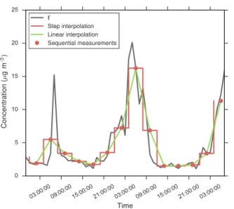
terpolation will better represent the original time series we have tested step interpolation as this case is often assumed (at least implicitly). For both interpolation cases we repre-sented a single measurement by the midpoint of a given sam-ple: each measurement occurs at timetmid=tstart+1τ/2=

tend−1τ/2). It is also possible to represent individual mea-surements by the start (tstart) or endpoints (tend) of each sam-ple. We do not consider those options here because the mod-eled results do not represent the original time series as well as the simulations withtmid.

3.2 Staggered sampling

Aerosol sample collection can also be staggered, such that each new sample is regularly initiated before termination of the previous sample. By separating successive measure-ments by a staggering interval δτ less than the individual sample-collection time 1τ, it is possible to increase mea-surement time resolution. The principle of combining multi-ple, overlapping, lower-resolution samples in order to con-struct higher spatial- and temporal-resolution information has been used extensively for image processing (Borman and Stevenson, 1998; Shechtman et al., 2005).

Staggered sampling effectively applies a running average to a time series of aerosol concentrations, which produces a smeared version of the original signal, denoted here asg(t ).

Iff (t )represents the true change in aerosol concentrations

at some point in the atmosphere from timet=0 toT,g(t )

is the product of the convolution of a boxcar kernel function

h(1τ )andf (t ). This is a specific example of a Fredholm

integral equation of the first kind:

g(t )=

T

Z

0

h(1τ )f (t )dt . (1)

In the case of measured data a smeared signal is more appropriately represented by a finite series of n

measure-ment pointsgseparated byδτ than by the continuous

func-tiong(t ). In addition, all measurements are subject to some

amount of measurement uncertaintyǫ. A discrete formula-tion of Eq. (1) that more accurately reflects the actual mea-surement process is the matrix equation:

g=Hf+ǫ, (2)

whereHis a convolution matrix andf is a finite series ofm

(5)

is the same as that ofg(i.e.,δτ). For staggered samples, the convolution matrixHis ann-by-mToeplitz matrix. Each of thenrows ofHcontains a shifted copy of a boxcar function

with k=1τ/δτ non-zero values equal to 1/ k. In general,

n=m+k−1. Figure 5 displays examples of a true time series

f of HOA concentrations and corresponding smeared time series without (Fig. 5a) and with (Fig. 5c) measurement error. Equation (2) suggests the following two post-processing methods for recovering a higher time resolution estimate _fˆ of the true time seriesf from staggered measurements.

1. The measured time series is taken as an approximation of the true time series. No further data processing is ap-plied.

2. One attempts to recover_fˆ _{through a deconvolution} op-eration. For example, ifH+is the pseudo-inverse matrix ofHone can solve the following inverse problem

ˆ

f =H+g. (3)

In principle, the true aerosol concentrationsf can be re-covered precisely from a set of staggered measurements g

and solution of Eq. (3) (Fig. 5b). However, in practice the problem is ill-posed. The small perturbations ǫtog due to random measurement uncertainty are strongly amplified in

ˆ

f. One can only ever hope to find a solutionfˆ that is a good

approximation off (Fig. 5d and e).

A variety of different deconvolution methods exist for finding the inverse solution of Eq. (2). For example, the con-volution theorem (Arfken and Weber, 2005) states that de-convolution amounts to simple division of the frequency do-main representations of f andH (which are typically ob-tained by Fourier and/orZ transforms). This deconvolution approach has recently been used to improve the time res-olution of slow response, broadband terrestrial irradiance measurements (Ehrlich and Wendisch, 2015). However, we choose to frame the deconvolution problem with the discrete matrix-based approach shown by Eq. (3) because it is well suited to the natural, discrete form of measurement data, does not assume periodicity of the time series being studies (as taking Fourier transforms would implicitly do), and allows easy and intuitive implementation of regularization methods (discussed in further detail below). For this work, we use a well-established and tested software package for inverse modeling by regularization (Regularization Tools Version 4.1 for MATLAB Hansen, 2007).

A further limitation of measured data relates to the extra

k measurement values at the boundaries ofg(recall for an

n-by-mHmatrix,n=m+k−1 wherek=1τ/δτ). These boundary elements correspond to partial samples with in-tegration times <1τ. In some experiments, it may be pos-sible to obtain the boundary values of g by initiating and concluding experiments with partial samples. However, this is not possible in experiments where1τ corresponds to the

lowest possible sampling time required to exceed the detec-tion limit. Therefore, only a truncated measurement vector

g_t withn−2(k−0.5)elements will be accessible for mea-surement in most cases (Fig. 4). There are two general ap-proaches for deconvolving a system withg_t.

1. Accept that the boundary values cannot be known and solve the resulting system of equations where H has more columns than rows, further adding to the ill-posedness of the problem. We refer to this as the trun-cated method for dealing with unknown boundary val-ues.

2. Pad the truncated measurement vectorg_t so that it has the same number of elements as the ideal, full con-volution productg. The resulting system of equations will be overdetermined, butgwill contain estimated (or guessed) values as well as actually measured values. For option (2), a variety of different padding methods ex-ist (e.g., Lane et al., 1997). Simple methods include the rep-etition of the final boundary values (uniform padding) or a reflection of the values about the boundaries (reflective padding). These padding methods are illustrated in Fig. 4. More refined methods concede that boundary conditions can-not be known a priori (e.g., Aristotelian boundary condi-tions, Calvetti et al., 2006). Here we consider only the simple methods of uniform and reflective padding and compare the results with those obtained from the truncated method (op-tion (1) above) and also from the ideal scenario where the full measurement vectorgis accessible for measurement.

To deal with the sensitivity of the solution to measurement uncertainty perturbations and the loss of boundary measure-ments some form of regularization is required. Regulariza-tion is the introducRegulariza-tion of addiRegulariza-tional informaRegulariza-tion in order to stabilize a solution. In this context, regularization can be achieved by modifying the convolution matrixHso that the components of the matrix that are responsible for explaining most of the variation in the underlying data are emphasized, while the components that are associated with high frequency measurement noise are deemphasized or removed. Regular-ization methods can be defined through the singular value decomposition (SVD) components ofH. SVD is also an im-portant practical tool for solving Eq. (3) (Hansen, 2007) and is defined as

H=U6VT, (4)

whereUis an m×mmatrix consisting of the left singular vectorsu1, . . . ,um,Vis an n×n matrix consisting of the

right singular vectorsv₁, . . . ,vn, and 6 is an m×n

diag-onal matrix consisting of diagdiag-onal elementsσi arranged in

descending order. Theσiare non-negative values and

(6)

03:00:00 09:00:00 15:00:00 21:00:00 03:00:00 09:00:00 15:00:00 21:00:00 03:00:00 Time

0 5 10 15 20 25

C

o

n

ce

n

tr

a

ti

o

n

(

µ

g

m

)

-3

f

Step interpolation

Linear interpolation

Sequential measurements

Figure 3.An illustrative example of interpolation between

sequen-tial samples. An original time seriesf of HOA concentrations, and

the time series resulting from step (red) and linear (yellow) interpo-lation between successive sequential samples, which are indicated by the circle markers.

For example, truncated SVD (TSVD) regularization is the most straightforward regularization method. TSVD in-volves retaining the first k SVD components of H, which

correspond to the largest singular valuesσi, and simply

dis-carding the rest. Tikhonov regularization is another common regularization method (Tikhonov and Arsenin, 1977). It in-volves minimizing a weighted sum of the residual and so-lution norms, with weighting parameter λ determining the importance given to the solution norm, or smoothness of the solution. The pseudo-inverse matrix is then defined by each method as (Aster et al., 2012)

H+=VkS−k1U T

k TSVD (5)

H+=(HTH+λI)−1HT Tikhonov, (6) where the subscript kindicates the number of components retained, andIis the identity matrix. As with TSVD, the ef-fect of Tikhonov regularization is to favor the large singu-lar values and deemphasize small singusingu-lar values. It can be seen that both regularization methods require the introduc-tion and setting of an addiintroduc-tional parameter:kfor TSVD and λfor Tikhonov regularization. Figure 5d and e illustrate how

critical it is to set the regularization parameter to an appro-priate value. If too many singular values are retained (large

k) or emphasized (smallλ), then the solution becomes highly unstable with strongly amplified perturbations. If too few sin-gular values are retained (smallk) or emphasized (largeλ), then the solution is overly smoothed.

2 0 2 4 6 8 10 12 14

Elapsed time (h)

0 2 4 6 8 10 12 14 16

C

oncent

rat

ion

(

µ

g m

)

-3

f g

gt

guni

gref

Figure 4.An original time seriesf of periodT =12 h measured

with 4 h samples (1τ=4 h) staggered at intervals of 1 h (δτ=1 h).

The resulting smeared signalgis the full convolution product of

f and a convolution matrixH(1τ, δτ ). Sincef contains 12 data

points,g contains 15(=12+(4/1)−1)data points. The values

at the boundaries ofgcorrespond to partial averages off

(sam-ples with sampling time <1τ). In practice these values are often not accessible for measurement, and one is left with a truncated measurement vectorg_tconsisting of only eight(=15−2(4−0.5))

data points. The truncated measurement vector can be padded on its edges by the uniform (g_uni) or reflective (g_ref) methods so that is has the same number of elements as the full convolution productg.

4 Description of the modeling

Numerical inverse modeling was conducted with the two test time series to compare the different methods of increasing time resolution (Fig. 2). Table 1 lists the model parameters and their values. The model parameters and values were cho-sen primarily to reprecho-sent aerosol sampling for FTIR spec-troscopy as detailed further below. However, the calculations are more general, and the results of the numerical modeling are applicable to any type of environmental sampling that can be characterized by parameters falling within the ranges indicated in Table 1.

We considered filter sampling periods of 4, 6, and 8 h. A minimum sample length of 4 h represents a typical value for the shortest possible sampling period required for aerosol FTIR spectroscopy (assuming the aerosol is not concentrated before sampling; if the sample is concentrated, FTIR sample-collection time can be as brief as 1 h, Maria et al., 2002). Se-quential sampling was modeled by averaging the true aerosol concentrations over sequential intervals of 1τ hours (e.g., circle markers in Fig. 3) centered at the sample midpoints. Staggered sampling with a staggering intervalδτ of 1 h was simulated by constructing a convolution matrixH(which de-pends on1τ) and evaluating Eq. (2).

(7)

en-[]

0 5 10 15 20

_(a)

f g, m=0 %

[]

0 5 10 15 20

_(b)

No regularization required

f ˆf

08:00:0014:00:0020:00:0002:00:0008:00:0014:00:0020:00:0002:00:0008:00:0014:00:00

Time

0 5 10 15 20

C

oncent

rat

ion

(

µ

g m

)

-3

(c)

f

g, m=20 %

[]

5 0 5 10 15 20 25

_(d)

TSVD regularization

f

ˆf, k=53 ˆfˆf, k=23, k=3

08:00:0014:00:0020:00:0002:00:0008:00:0014:00:0020:00:0002:00:0008:00:0014:00:00

5 0 5 10 15 20 25

_(e)

Tikhonov regularization

f

ˆf, λ=0.1 ˆfˆf, λ=0.39, λ=1

Figure 5.Explanation of different types of time series:fis an original time series of HOA concentrations;gare smeared time series produced

from the staggering of 4 h samples (1τ=4 h) at 1 h intervals (δτ=1 h)(a)without (κm=0 %) and(c)with the addition of normally

distributed random measurement error (κm=20 %). The right panels contain time seriesfˆ recovered by deconvolution of the smeared

time seriesgin the corresponding left panels. Whenκm=0 %(b), the true time series can be completely recovered by deconvolution. No

regularization is required. Whenκm=20 %,(d)TSVD regularization with appropriate choice ofk(=23), or(e)Tikhonov regularization

with appropriate choice ofλ(=0.39)are required to obtain solutions that approximate the true time series well.

Table 1.Modeling parameters

Parameter Description Value(s)

1τ(h) Sample collection or measurement integration time 4, 6, 8

δτ(h) Staggering interval 1

T (h) Period of time series being measured 12, 19, 38, 57, 76, 114, 228

κm(% of mass) Relative measurement error 0, 1, 5, 10, 20, 30

σ₀,m(µg) Fixed or blank measurement error 0.5

sure that the same, full, 228-hour-long HOA and OOA time series were used for each value ofT, multiple time series

seg-ments were modeled for eachT < 228 h, and the results are

reported as averages over these multiple segments. For ex-ample, forT =12 h, 19(=228/12) separate time series seg-ments were modeled. ForT =228 h only a single HOA and a single OOA input time series were required.

Initial testing indicated that the start time of a series of sequential samples affected the ability of the resulting mea-surement signal to represent the true aerosol concentrations. For example, if a long filter sample is initiated at the apex

(8)

For1τ =6 h, six unique sequential sampling schedules were possible, and for1τ =8 h, eight unique schedules were pos-sible.

For both the sequential and staggered cases perturbations due to random measurement error (ǫ, see Eq. (2) were added to the simulated measurements. Relative measurement errors (κm) of 0, 1, 5, 10, 20 and 30 % were considered. A relative

measurement error of 20 % is typical for aerosol FTIR spec-troscopy (Russell, 2003). The relative errors were applied to aerosol mass, not concentration, since this is the quantity ac-tually probed by FTIR spectroscopy (we use the subscriptm

to denote mass units). A sampling flow rate of 10 L min−1 was multiplied by the given sampling intervals1τ to

calcu-late the sampling volumes used to convert between mass and concentration. We assumed that the relative error in the mea-surement of sampling flow rate was 2 %. The relative error in the measurement of the sampling time interval1τ was as-sumed to be so small in comparison to the errors in measured mass and flow rate that it could be neglected. The relative un-certainties in measured mass and flow rate were summed in quadrature to calculate total, relative uncertainty in aerosol concentration, denoted asκc, where the subscriptcindicates

concentration units.

The relative error was combined with a fixed error term (σ0,m). The fixed error term represents, for example, the

stan-dard deviation of masses detectable on blank filter samples. The fixed error term is typically on the order of 0.1 µg for aerosol FTIR samples on Teflon filters. We conservatively setσ0,mto 0.5 µg, which is at the upper end of the range of

blank uncertainty values measured in previous FTIR studies (Maria et al., 2003; Gilardoni et al., 2009, 2007). A fixed error of 0.5 µg is consistent with the selected minimum sam-pling interval of 4 h (Table 1). Defining detection limit as 3σ0,m, 4 h of sampling would be required to ensure that

al-most all (> 97 %) of the organic functional group samples representing HOA and OOA collected during the time period covered by the test time series were above detection limit (Fig. S1 in the Supplement). We also modeledσ0,m=0.1 µg.

The results were insensitive to this change so are not included here.

Taking the relative and fixed errors, total measurement er-rorσas a function of concentrationcwas calculated with the

linear error model described by Eq. (7). Linear dependance of total measurement error on concentration is a widely ap-plicable assumption (e.g., Ripley and Thompson, 1987).σ0,c

is in units of concentration and is therefore a function of a given1τ and the sampling flow rate. The concentration per-turbationsǫdue to the total measurement error were assumed to be normally distributed around a mean of 0 withσ repre-senting 1 standard deviation of the distribution:

σ (c)=κcc+σ0,c (7)

ǫ∼N(0, σ (c)). (8)

By setting the means of theǫdistributions to 0 we have as-sumed that the simulated measurements are not affected by systematic measurement artifacts. Systematic measurement artifacts depend strongly on the measurement technique in question and even the specific batch of materials used (e.g., filter lot). They can be positive or negative, and can depend on sampling time (e.g., Kirchstetter et al., 2001; Subrama-nian et al., 2004). If known, measurement artifacts could be addressed in this modeling framework by the setting the means of theǫdistributions to non-zero, time-dependant val-ues.

Forκm= 0 %,σ(c) and henceǫwere set to 0 to represent

the ideal case of absolutely no perturbations due to measure-ment error. For each modeling run with non-zeroκm, 20

dif-ferent realizations of the randomly generated error perturba-tionsǫwere generated and added to the measurement signal. Results are reported as averages over the 20 different realiza-tions of each noisy measurement signal.

Hourly resolved time series were constructed from the simulated measurement signals using the post-processing methods outlined in Fig. 2 as follows. The sequential-interpolated solutions were constructed by interpolating be-tween sequential data points at the chosen resolution of 1 h with step and linear functions. The smeared solutions re-quired no further data processing: the time series g pro-duced by simulating staggered sampling were taken as is. The deconvolution solutions were obtained by first modi-fying the simulated measurement vectors according to the chosen boundary value method: full – the full measurement vectors were used in subsequent calculations; truncated – values at the boundaries of the measurement vectors corre-sponding to partial samples were removed (and a correspond-ing truncated convolution matrixHr was calculated by

re-moving rows inHcorresponding to these boundary values); uniformly and reflectively padded – boundary values corre-sponding to partial samples were removed but the measure-ment vector was then padded back to the original length ofg

(9)

Inves-tigation of these methods is beyond the scope of this work, but it must be stressed that less accurate solutions would be obtained with these parameter choice methods than with the optimal, RMSE-minimizing method employed here.

The post-processing methods for increasing time resolu-tion were judged according to two criteria:

1. Recovery error (RE): the overall ability to recover the true time series from a set of simulated measurements. We define RE as the mean absolute error (MAE) be-tween a given calculated, hourly resolved time series_fˆ consisting ofndata points and the corresponding true, original time seriesf:

RE=MAE=1 n

n

X

i=1

| ˆf_i−f_i|. (9)

RE is the combination of two types of errors: the error due to the measurement noise simulated by the linear error model described by Eq. (7) (which we denote as Measurement Error, ME), and the error resulting from increasing the measurement time resolution from 4, 6, or 8 h to 1 h via one of the post-processing methods. We denote this latter error as upsampling error, UE (upsam-pling is a signal processing term used to describe the use of interpolation to increase the resolution of a sig-nal; our use of the term here is not strictly applied to interpolation, but to methods of increasing resolution in general). UE can be calculated by the following equa-tion

UE=RE−ME=RE−1 n

n

X

i=1

|f_i−f′_i|, (10)

where ME is defined as the mean absolute error between a true time seriesf consisting of ndata points and a time series f′ produced by a hypothetical instrument subject to the same random error modeled by our linear error model, but capable of measuring at hourly rather than 4–8 h time resolution. We choose to report the bulk of the results as RE to represent the total error result-ing from the upsamplresult-ing of noisy measurements. In the final discussion Sect. 9 we also report typical UEs to illustrate how much of the total error can be attributed solely to the upsampling process.

2. Peak capture: the specific ability to recover the magni-tude and timing of the daily concentration peaks (indi-cated by the circle markers in Fig. 1). The ability of a method to accurately capture peaks in concentration is important for health and regulatory concerns (e.g., for identifying exceedances of particulate matter air quality guidelines). We assess peak capture through a peak plot, which displays the mean difference between the daily peak concentrations in a calculated hourly resolved time series and the corresponding peak concentrations in the

true time series, against the mean difference between the times that the peaks occur in the calculated time series and in the corresponding true time series.

In the discussion of the modeling results we pay particular attention to the measurements of 57 h-long time periods with 4 h samples subject to 20 % measurement error. This repre-sents a typical FTIR experiment. However, the dependance of recovery error on time-series period, filter sample length, and the level of measurement error is also discussed.

5 Sequential sampling results

This section identifies the best representation (step or linear) of atmospheric concentrations using sequential samples and discusses the issue of sequential sampling schedule. These questions are answered with reference to overall recovery er-ror (RE, Sect. 4) since the ability to capture peak concentra-tions with sequential samples does not depend on the inter-polation method employed (unless higher order interinter-polation functions are used).

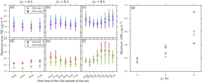
Figure 6a–f shows the dependance of RE on the start time of the second sample of the day for HOA and OOA time series that were constructed by step and linear interpolation between sequential samples of sampling length (1τ) 4, 6, and 8 h (T =57 h andκm=20 %). The start time of the sec-ond sample of the day represents sample schedule. For both HOA and OOA, RE is generally lower for the linearly in-terpolated solutions than the step inin-terpolated solutions, and RE increases with increasing1τ. Figures S2 and S3

indi-cate that linear interpolation results in lower recovery error than step interpolation over the full ranges of simulated time-series periods and relative measurement errors, respectively. Therefore not surprisingly, linear interpolation is a more ef-fective method for post-processing sequential measurement than step interpolation.

Figure 6g plots the maximum difference in RE between two different sampling schedules (designated as maximum

(10)

[] 0.5

1.0 1.5 2.0 2.5 3.0 3.5

[]---∆τ = 4 h

(a) HOA step

HOA linear

[]

∆τ = 6 h

(b)

[]

∆τ = 8 h

(c)

04:00 05:00 06:00 07:00

[] 1.5

2.0 2.5 3.0 3.5 4.0

R

e

c

o

v

e

ry

erro

r,

R

E

(

µ

g

m

)

(d) OOA step

OOA linear

06:0007:0008:0009:0010:0011:00 Start time of the 2nd sample of the day

[]

(e)

08:0009:0010:0011:0012:0013:0014:0015:00

[]

(f)

4 6 8

∆τ (h)

0.0 0.2 0.4 0.6 0.8 1.0

Ma

x

imu

m

∆

R

E

(

µ

g

m

)

-3

(g)

-3

Figure 6. (a)–(f)Mean recovery error (RE) as a function of the start time of the second sample of the day for HOA and OOA time series

constructed by step and linear interpolation between sequential measurements of length (1τ) 4, 6, and 8 h.κm=20 % andT =57 h, meaning

each data point is an average over 4(=228/57) time series segments. The start time of the second sample of the day represents the 4, 6, and 8 unique sequential sampling schedules that are possible with 4, 6, and 8 h samples, respectively (Sect. 4). The vertical bars represent 95 %

confidence intervals determined by bootstrapping the mean estimates.(g)Maximum1RE vs.1τ. Maximum1RE represents the maximum

difference in RE between two unique sampling schedules for a given1τ. It is the maximum possible potential error that may be incurred if

a suboptimal sampling schedule is chosen for a given type of time series.

times > 6 h. This scheduling effect is not as important for staggered samples, assuming the staggering interval is small enough, since measurement data points are collected more frequently.

6 Deconvolution results

Eight different combinations of regularization and bound-ary value methods (Fig. 2) were used to recover time series by deconvolution for each set of simulated staggered mea-surements. ForT =57 h andκm=20 %, Fig. 7 displays the

mean RE of deconvolution solutions recovered by TSVD and Tikhonov regularization as a function of the boundary value method employed (tiled by 1τ and time series type), and Fig. 8 displays a peak plot for each combination of regular-ization and boundary value method.

At this relatively high level of measurement error, only a small reduction in RE is gained from having access to the full measurement vector (which would require the collection of partial samples, Sect. 3). Furthermore, there is little differ-ence in the mean RE of the three methods that assume bound-ary values are not accessible for measurement: no clear and consistent advantage can be discerned between the truncated, uniformly, and reflectively padded methods for this T and

κm. Assuming the boundary values are known, the average

RE of HOA time series sampled with 4 h filters and recov-ered with TSVD regularization is 1.16 µg m−3_{. If the} bound-ary values are not known, the corresponding value averaged over the three other boundary value methods is 1.34 µg m−3_.

The corresponding OOA-TSVD results tell the same story: RE of 1.42 µg m−3 _{with the full measurement vector vs. an} average of 1.65 µg m−3_{over the three methods without. The} results are similar over the full range of time-series periods simulated (Fig. S4).

In addition, at this level of measurement error similar re-covery errors are obtained with TSVD and Tikhonov regu-larization. It is only for the OOA time series measured with 4 h samples that a difference between the two regularization methods can be clearly discerned, with TSVD regularization resulting in lower recovery error than Tikhonov regulariza-tion. Although the REs are similar, concentrations recovered with Tikhonov regularization are generally lower than the true concentrations. As a result, the overall average concen-trations of time series recovered with Tikhonov regulariza-tion are 10–20 % below the corresponding averages of the original time series. The average concentrations of the time series recovered with TSVD regularization are very similar to the true values (Fig. S6).

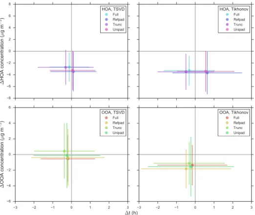
The peak plots (Fig. 8) indicate that in terms of peak cap-ture no boundary value method is clearly better than the oth-ers forκm=20 %. Solutions with TSVD regularization are

(11)

[] 0.5

1.0 1.5 2.0 2.5 3.0

[]

∆τ

= 4 h

HOA Tikhonov HOA TSVD

[]

∆τ

= 6 h

[]

∆τ

= 8 h

Full Trunc Unipad Refpad

[] 1.0

1.5 2.0 2.5 3.0 3.5

R

e

co

ve

ry

erro

r,

R

E

(

µ

g

m

)

-3

OOA Tikhonov OOA TSVD

Boundary value method

[]

Figure 7.Mean recovery error (RE) for different boundary value methods for HOA and OOA time series constructed by deconvolution with

TSVD and Tikhonov regularization of staggered measurements of length (1τ) 4, 6, and 8 h.κm=20 % andT =57 h, meaning each data

point is an average over 4(=228/57) time series segments. The boundary value methods are full; trunc, truncated; unipad, uniformly padded; and refpad, reflectively padded. The vertical bars represent 95 % confidence intervals determined by bootstrapping the mean estimates.

2 µg m−3_{. The daily HOA and OOA peak times can generally} be reproduced to within 1 h.

If the level of random measurement error is very low, less than approximately 5 %, recovery error is strongly reduced if one has access to the full measurement vector (Fig. S5). If partial samples cannot be known, solving the system of equa-tions with a truncated measurement vector results in lower er-ror than padding the measurements out via the uniform or re-flective methods. Taking all of these together we recommend TSVD regularization with the truncated method for dealing with boundary values if partial samples cannot be known. In addition to the analysis presented in this work, further advan-tages of TSVD regularization are that it is conceptually sim-ple and intuitive, and it is straightforward to apply through the SVD products of the convolution matrixH.

7 Overall comparison of methods

Based on the findings of the previous two Sects. 5 and 6 we now make an overall comparison of methods for increasing measurement time resolution in the context of the practical considerations and limitations of each method. Interpolation between sequential measurements is the least sophisticated, cheapest and easiest of the methods for increasing time res-olution out of those that we have investigated. Staggered sampling requires multiple sampling lines to collect multi-ple sammulti-ples at once. More staggered sammulti-ples are required to

cover a given time period than would be required to cover the same time period with sequential samples. This extra cost of staggered sampling compared to sequential sampling is illus-trated in Fig. 9. For example, to measure a time series of pe-riod 64 h, 61 staggered 4 h samples would be required com-pared to only 16 sequential 4 h samples. The sample number difference is even greater for larger1τ. To measure a time

series of period 64 h, 57 staggered 8 h samples would be re-quired compared to only 8 sequential 8 h samples.

Attempting to recover the true time series from a set of staggered measurements by deconvolution requires even fur-ther effort and analysis time and expertise. Although tried and tested deconvolution and regularization algorithms are readily available (Hansen, 2007), the choice of a reasonable regularization parameter may not be straightforward. If a bad regularization parameter is chosen, a substantial additional error could be added to a solution (Fig. 5). Given the extra cost of staggered sampling and the error risk associated with regularization, it is necessary to establish precisely what, if anything, can be gained from the use of these more sophis-ticated tactics for a variety of different experimental condi-tions.

Figure 10 displays the mean recovery error as a func-tion of κm for HOA and OOA time series processed by

(12)

low-[] 8

6 4 2 0 2 4 6 8

∆

HO

A

co

nce

ntra

tio

n (

µ

g m

−

3)

HOA, TSVD

Full Refpad Trunc Unipad

[]

HOA, Tikhonov

3 2 1 0 1 2 3

∆t (h) 6

4 2 0 2 4 6

∆

OO

A

co

nce

ntra

tio

n (

µ

g m

−

3)

OOA, TSVD

3 2 1 0 1 2 3

[]

OOA, Tikhonov

Figure 8. Peak plots for time series of period 57 h measured with 4 h samples subject to 20 % measurement uncertainty recovered by

each of the eight combinations of regularization (TSVD, Tikhonov) and boundary value (full, trunc:truncated, unipad:uniformly padded,

refpad:reflectively padded) methods. The peak plots are explained fully in the main text in Sect. 4. Briefly,1[HOA or OOA] concentration

represents the mean difference in daily peak concentrations and1t the mean difference in daily peak timing between a calculated, hourly

resolved time series and its corresponding true time series. The vertical and horizontal bars represent 1 standard deviation of the1[HOA or OOA] concentration and1t results, respectively, for each daily peak in all of the modeled solutions.

0 50 100 150 200 250

Time series period, T (h)

0 50 100 150 200 250

Nu

mb

er

of

sa

mp

les,

N

Sequential, ∆τ =4 h

Staggered, ∆τ =4 h

Sequential, ∆τ=6 h

Staggered, ∆τ=6 h

Sequential, ∆τ=8 h

Staggered, ∆τ=8 h

Figure 9.The number of filter samplesN of length 4, 6, and 8 h

required to measure time series of periodTh sequentially and by

staggering the samples at an intervalδτ of 1 h. The number of

se-quential samples is given by T /1τ and the number of staggered

samples is given by(T−1τ+1)/δτ.

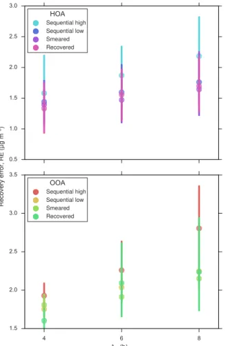
est RE, and “sequential high” corresponds to the sampling schedule that resulted in the highest RE. The RE difference between these two cases is the sequential sampling effect identified in Fig. 6g. The recovered solutions were produced by deconvolution with TSVD regularization and the trun-cated method for dealing with inaccessible boundary values (Sect. 6). As expected, in the absence of measurement error, recovering a time series through the deconvolution of stag-gered measurements is the best method for achieving high time resolution. On average, true concentrations can be re-produced to within 0.25 µg m−3 _{for HOA and 0.48 µg m}−3 for OOA with this method (RE is not zero because of the truncated measurement vector). However, measurement er-ror is unavoidable, and the presence of only 5 % erer-ror is suf-ficient for the recovered method to lose its RE advantage over the less sophisticated sequential and smeared methods.

(13)

[]

0.0 0.5 1.0 1.5 2.0 2.5 3.0

[]

HOA

Sequential high Sequential low Smeared Recovered

0 5 10 15 20 25 30

Relative measurement error, m (%)

0.0 0.5 1.0 1.5 2.0 2.5 3.0

R

e

co

ve

ry

erro

r,

R

E

(

µ

g

m

)

-3

OOA

Figure 10. Mean recovery error (RE) against relative

measure-ment error for HOA and OOA time series processed by the

se-quential, smeared and recovered methods.T =57 h and1τ=4 h.

The “sequential high” and “sequential low” time series are con-structed by linear interpolation between suboptimally and optimally scheduled sequential measurements, respectively. The recovered so-lutions were obtained with TSVD regularization and the truncated boundary method.

sampling schedule is chosen, mean RE for the HOA time se-ries could be as high as 1.58 µg m−3_{. In a real experiment} there would be no way of knowing what the optimal sequen-tial sampling schedule was (unless a complementary inde-pendent measurement was available), and therefore whether a sequentially measured time series would be subject to the higher amount of error or not. Collecting staggered samples is one option for avoiding the sample scheduling effect.

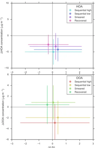
The peak plots corresponding to the REs shown in Fig. 10 for κm=20 % are displayed in Fig. 11. Both the optimally

and suboptimally scheduled sequential solutions are slightly worse at capturing peak concentrations then the smeared and recovered solutions. For example, peak HOA concentrations are underestimated by an average of 4.28 µg m−3_{in the} op-timally scheduled sequential solution compared to 3.32 and 2.74 µg m−3_{for the smeared and recovered solutions} respec-tively. For the OOA time series, peak concentration values

3 2 1 0 1 2 3

10 5 0 5 10

∆

HO

A

co

nce

ntra

tio

n (

µ

g m

−

3)

HOA

3 2 1 0 1 2 3

∆t (h)

6 4 2 0 2 4 6

∆

OO

A

co

nce

ntra

tio

n (

µ

g m

−

3)

OOA

Figure 11.Peak plots for time series of period 57 h measured with

4 h samples subject to 20 % measurement uncertainty processed by the sequential, smeared and recovered methods. The “sequen-tial high” and “sequen“sequen-tial low” time series are constructed by lin-ear interpolation between suboptimally and optimally scheduled se-quential measurements, respectively. The recovered solutions were obtained with TSVD regularization and the truncated boundary method. The peak plots are explained fully in the main text in Sect. 4.

are reproduced, on average, very accurately in the smeared and recovered solutions, being overpredicted by only 0.85 and 0.43 µg m−3_{, respectively. The same peak concentrations} are underestimated by 1.94 µg m−3 _{in the optimally} sched-uled sequential solution.

A key variable included in our numerical model is the fil-ter sample length1τ. Figure 12 displays mean RE against

1τ for the same cases shown in Figs. 10 and 11. Again

T =57 h andκm=20 %. It is interesting to note that mean

(14)

[] 0.5

1.0 1.5 2.0 2.5 3.0

[]

HOA

4 6 8

∆τ (h) 1.5

2.0 2.5 3.0 3.5

R

e

c

o

v

e

ry

er

ro

r,

R

E

(

µ

g

m

)

-3

OOA

Figure 12. Mean recovery error (RE) against sample-collection

time for HOA and OOA time series processed by the sequential,

smeared and recovered methods. T =57 h and κm=20 %. The

“sequential high” and “sequential low” time series are constructed by linear interpolation between suboptimally and optimally sched-uled sequential measurements, respectively. The recovered solu-tions were obtained with TSVD regularization and the truncated boundary method.

error is only slightly greater, 2.15 µg m−3_{. However in the} case of suboptimally scheduled sequential measurements the increase in RE with1τ is considerably greater because the sequential sampling scheduling effect increases with increas-ing sample-collection time (Fig. 6g).

Whether or not the differences between the sequential, smeared and recovered methods are significant depends on the specific aims of a given experiment. If the priority is to achieve low overall error over long time periods when mea-suring a concentration time series with 4 h samples subject to 20 % relative measurement error, linear interpolation be-tween sequentially collected samples is likely to be a suitable enough choice for achieving hourly time resolution. Addi-tional error may be inadvertently introduced through choice of a suboptimal sampling schedule but the extra practical costs of staggered sampling (Fig. 9) would be avoided. On the other hand, if one was particularly interested in accurately

measuring peak OA concentrations and had the ability to run multiple sampling lines at once, then staggered sampling with no further data processing would be the best option for achieving hourly time resolution (Fig. 11). A combination of sequential sampling during stable OA concentration periods and staggered sampling during peak periods (e.g., morning rush hours, afternoon peak in photochemistry) could be an excellent strategy for intensive field campaigns.

Our analysis suggests that in scenarios similar to the case studied in this work there is little benefit to be gained (in terms of both overall error and peak capture) by running staggered measurements through a deconvolution algorithm. This is surprising given that in the absence of perturbations to a measurement signal, true concentrations can be recovered precisely from a set of staggered measurements (Fig. 5b). However, once non-ideal, practical realities such as random measurement error (even as low as 5 %) and the inability to collect partial samples are taken into account, signals recov-ered by deconvolution approximate true concentrations only as well as smeared and interpolated signals, even with opti-mal choice of regularization parameter. Considering that in a real experiment the optimal regularization parameter is not known, we do not recommend the deconvolution of staggered measurements as a method for increasing time resolution, un-less the level of relative measurement error is extremely low (< 1 %).

8 Comparison of HOA and OOA results

(15)

9 Interpretation of errors

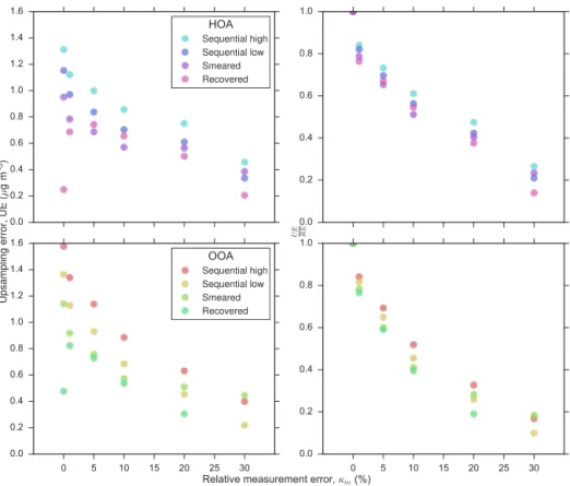
The REs (Eq. 9) we have reported indicate to within what concentration range one can measure true aerosol concen-trations, on average, with hourly resolved time series con-structed from noisy measurement samples of length 4–8 h. These REs are a combination of random measurement er-ror (ME, which we modeled with the linear erer-ror model de-scribed by Eq. (7) and upsampling error (UE), as explained in Sect. 4. UE represents the error associated solely with the increase in time resolution from 4–8 to 1 h. UE can be calcu-lated with Eq. (10).

To illustrate how the errors break down for the caseT = 57 h and1τ =4 h, Fig. 13 displays the upsampling errors, and the UE fractions of the total error as a function of κm

for HOA and OOA time series constructed for the sequen-tial high and low, smeared and recovered cases. In each case, the UE/RE fraction decreases substantially with increasing

κm from 76–84 % at κm=1 % to 10–27 % at κm=30 %.

For the sequential and smeared cases this is because UE de-creases and ME inde-creases with increasingκm. For the

recov-ered case, absolute UE is less dependent onκm(it is always

less than 0.83 µg m−3_{), and the decreasing UE}_/_{RE fraction} results mainly from the increase in ME with increasingκm.

The inverse relationship between UE/RE andκm indicates

that although total recovery error decreases with an increase in analytical accuracy (decrease inκm, Fig. 10), the fraction

of the total error resulting from the upsampling process in-creases.

For FTIR levels of relative measurement error of 20 %, UEs represent only 19–47 % of total RE in the sequen-tial, smeared and recovered cases. In absolute terms, 0.30– 0.75 µg m−3_{of error can be attributed specifically to the} pro-cess of constructing an hourly resolved time series from a set of 4 h samples. This means that if FTIR sample collec-tion was improved so that it was possible to collect samples over 1 h instead of 4 h, the precision of the resulting hourly resolved measurements would be improved by only 0.30– 0.75 µg m−3_{, relative to hourly resolved time series} con-structed from 4 h samples (the accuracy of the measurement will depend on the analytical bias and measurement artifacts of the technique in question). This statement is true even for the simple case of linear interpolation between suboptimally scheduled sequential measurements. This absolute upsam-pling error range represents only 1.7–4.7 % of the average daily HOA and OOA peak concentrations, and 3.7–15.2 % of the average of all HOA and OOA concentrations in the test time series (Fig. 1).

One way to frame these errors is to consider each com-bination of noisy 4–8 h measurement samples and post-processing method as a self-contained measurement tech-nique or instrument that measures OA concentrations at hourly resolution. For example, submicrometer size dis-tributions measured with a scanning mobility particle sizer (SMPS) are typically considered as a standard,

self-contained measurement. In fact, SMPS measurements are a combination of particle electrical mobility measurements and an inversion algorithm. SMPS inversion algorithms are analogous to the post-processing methods we have tested here, and are even based on the same underlying mathemat-ics of deconvolution (e.g., Pfeifer et al., 2014), although it is not necessary for the modern SMPS user to know this fact. In this framing, the total error of each hourly resolved OA con-centration measurement (RE) can be considered as a combi-nation of random error in the underlying measurement (ME) and error introduced by the processing algorithm (UE). UE is the error cost of increasing the measurement time resolution. Taking this interpretation further, one can also use esti-mated concentrations to characterize the equivalent bias and error of the hourly-resolution measurements as a whole, anal-ogously to the way bias and error would be characterized for any new instrument. An example of equivalent bias and er-ror characterization is provided in Sect. S5 for the sequen-tial high and low, smeared, and recovered cases considered in Sect. 7. We have not quantitatively characterized equiva-lent errors for these cases because Fig. S7 indicates that the post-processing methods alter the structure of the errors in the estimated concentrations, and the linear error model de-scribed by Eq. (7) is no longer applicable. Therefore, further work would be required to find a more suitable error model and to quantify equivalent error. However, the example still demonstrates how the hourly resolved outputs of the post-processing methods that we have tested can be treated in the same manner as the output of any given instrument or mea-surement technique.

10 Conclusions

Aerosol measurement techniques with high analytical de-tection limits require long sample-collection times at atmo-spherically relevant concentrations, which results in poorly time-resolved measurements. We investigated combined sampling and post-processing methods for increasing the res-olution of time series produced with 4–8 h-long samples. The absolute concentrations we sought to recover ranged from 0.13 to 29.16 µg m−3 _{with mean values of 4.99 (HOA) and} 8.09 µg m−3 _{(OOA) (Fig. 1). Linear interpolation between} sequentially collected samples is cheap, simple and surpris-ingly effective in terms of both overall recovery error and daily peak capture. However, sequential samples are subject to a sample schedule effect, which can add up to 0.56 µg m−3 to overall recovery error (Fig. 6). Staggered sampling avoids the sample schedule effect and it is up to the experimenter to decide if the extra practical costs of staggered sampling (e.g., Fig. 9) are worth this benefit. Recovering a time se-ries through deconvolution of staggered measurements is only useful at low values of relative measurement error. For

κm> 5 % the recovery errors of recovered solutions are

(16)

[]

0.0 0.2 0.4 0.6 0.8 1.0 1.2 1.4 1.6

[]

HOA

[]

0.0 0.2 0.4 0.6 0.8 1.0

[]

0 5 10 15 20 25 30

Relative measurement error, m (%)

0.0 0.2 0.4 0.6 0.8 1.0 1.2 1.4 1.6

U

p

s

a

m

p

lin

g

er

ro

r,

U

E

(

µ

g

m

)

-3

OOA

0 5 10 15 20 25 30

[]

0.0 0.2 0.4 0.6 0.8 1.0

UE RE

Figure 13.Left panels: upsampling error (UE) vs.κmfor HOA and OOA time series (T =57 h) measured with 4 h samples. Right panels:

the corresponding UE fractions of the total error (RE) as a function ofκm.

Since deconvolution costs extra analysis time and expertise, and there is a risk that further error can be added to a solution through the bad choice of regularization parameter, we do not recommend this approach for post-processing staggered measurements in scenarios similar to the case studied in this work. If a deconvolution algorithm is applied, we recom-mend using TSVD regularization because it resulted in more accurate average concentrations over full sampling periods, and marginally better peak capture and REs than Tikhonov regularization.

Our numerical modeling has indicated that forκm=20 %, one can measure concentrations to within a range of 1.33– 2.25 µg m−3_{, on average, with hourly resolved time series} constructed from samples of length 4–8 h using the best-case sequential, smeared or recovered methods. Daily peak con-centrations can be reproduced to within an average of 0– 4.3 µg m−3_{and peak times can be reproduced to within an} hour. Surprisingly, for the caseT =57 h and1τ=4 h, only 19–47 % of the overall recovery error can be attributed to the actual upsampling process. In absolute terms, this indi-cates that measurement precision would only be improved by 0.30–0.75 µg m−3_{if samples could be collected over 1 h} instead of 4 h.

The total and upsampling errors we have reported rep-resent only small fractions of the average daily peak con-centrations in the HOA and OOA test time series.

There-fore, post-processing methods are effective techniques for in-creasing the time resolution of OA measurements requiring long sample-collection times. Application of these methods should be considered as a good alternative or complement to other methods of achieving high time resolution, such as in-strument redesign for rapid sample collection, which in many cases may be prohibitively expensive.

These conclusions are based on the two time series we have investigated, which included sharp (high gradients), broad (low gradients), large magnitude, and relatively flat regions (Fig. 1). However, further work is required to test the generality of the conclusions by applying these sampling strategies and post-processing methods to different time se-ries types (e.g., cooking organic aerosols, which may display even sharper peaks in concentrations). The theoretical and modeling frameworks provided in Sects. 3 and 4 do not de-pend on the specific test case in question and can be applied to time series of any variable.

(17)

Acknowledgements. The authors thank J. L. Jimenez for providing

the aerosol mass spectrometry data, V. M. Panaretos for interesting and informative discussions on inverse problems and the treatment of boundary values, and EPFL for funding. R. L. Modini acknowl-edges support from the “EPFL Fellows” fellowship programme co-funded by Marie Curie, FP7 Grant agreement no. 291771.

Edited by: H. Herrmann

Reviewed by: two anonymous referees

References

Aiken, A. C., Salcedo, D., Cubison, M. J., Huffman, J. A., DeCarlo, P. F., Ulbrich, I. M., Docherty, K. S., Sueper, D., Kimmel, J. R., Worsnop, D. R., Trimborn, A., Northway, M., Stone, E. A., Schauer, J. J., Volkamer, R. M., Fortner, E., de Foy, B., Wang, J., Laskin, A., Shutthanandan, V., Zheng, J., Zhang, R., Gaffney, J., Marley, N. A., Paredes-Miranda, G., Arnott, W. P., Molina, L. T., Sosa, G., and Jimenez, J. L.: Mexico City aerosol analysis during MILAGRO using high resolution aerosol mass spectrom-etry at the urban supersite (T0) – Part 1: Fine particle composi-tion and organic source apporcomposi-tionment, Atmos. Chem. Phys., 9, 6633–6653, doi:10.5194/acp-9-6633-2009, 2009.

Arfken, G. B. and Weber, H.-J.: Mathematical Methods for Physi-cists, Elsevier, Burlington, MA, USA, 951–952, 2005.

Aster, R., Borchers, B., and Thurber, C.: Parameter Estimation and Inverse Problems, Academic Press, Waltham, MA, 2nd ed., ISBN-13: 978-0-12-385048-5, 2012.

Borman, S. and Stevenson, R.: Spatial Resolution Enhancement of Low-Resolution Image Sequences – A Comprehensive Review with Directions for Future Research, Tech. rep., 1998.

Calvetti, D., Kaipio, J. P., and Someralo, E.: Aristotelian prior boundary conditions, Int. J. Math. Comp. Sci., 63–81, 2006. Corrigan, A. L., Russell, L. M., Takahama, S., Äijälä, M., Ehn,

M., Junninen, H., Rinne, J., Petäjä, T., Kulmala, M., Vogel, A. L., Hoffmann, T., Ebben, C. J., Geiger, F. M., Chhabra, P., Seinfeld, J. H., Worsnop, D. R., Song, W., Auld, J., and Williams, J.: Biogenic and biomass burning organic aerosol in a boreal forest at Hyytiälä, Finland, during HUMPPA-COPEC 2010, Atmos. Chem. Phys., 13, 12233–12256, doi:10.5194/acp-13-12233-2013, 2013.

de Gouw, J. A., Welsh-Bon, D., Warneke, C., Kuster, W. C., Alexan-der, L., Baker, A. K., Beyersdorf, A. J., Blake, D. R., Cana-garatna, M., Celada, A. T., Huey, L. G., Junkermann, W., Onasch, T. B., Salcido, A., Sjostedt, S. J., Sullivan, A. P., Tanner, D. J., Vargas, O., Weber, R. J., Worsnop, D. R., Yu, X. Y., and Za-veri, R.: Emission and chemistry of organic carbon in the gas and aerosol phase at a sub-urban site near Mexico City in March 2006 during the MILAGRO study, Atmos. Chem. Phys., 9, 3425– 3442, doi:10.5194/acp-9-3425-2009, 2009.

Decesari, S., Fuzzi, S., Facchini, M. C., Mircea, M., Emblico, L., Cavalli, F., Maenhaut, W., Chi, X., Schkolnik, G., Falkovich, A., Rudich, Y., Claeys, M., Pashynska, V., Vas, G., Kourtchev, I., Vermeylen, R., Hoffer, A., Andreae, M. O., Tagliavini, E., Moretti, F., and Artaxo, P.: Characterization of the organic com-position of aerosols from Rondônia, Brazil, during the LBA-SMOCC 2002 experiment and its representation through model

compounds, Atmos. Chem. Phys., 6, 375–402, doi:10.5194/acp-6-375-2006, 2006.

Ehrlich, A. and Wendisch, M.: Reconstruction of high-resolution time series from slow-response broadband terrestrial irradiance measurements by deconvolution, Atmos. Meas. Tech., 8, 3671– 3684, doi:10.5194/amt-8-3671-2015, 2015.

Finessi, E., Decesari, S., Paglione, M., Giulianelli, L., Carbone, C., Gilardoni, S., Fuzzi, S., Saarikoski, S., Raatikainen, T., Hillamo, R., Allan, J., Mentel, Th. F., Tiitta, P., Laaksonen, A., Petäjä, T., Kulmala, M., Worsnop, D. R., and Facchini, M. C.: Determi-nation of the biogenic secondary organic aerosol fraction in the boreal forest by NMR spectroscopy, Atmos. Chem. Phys., 12, 941–959, doi:10.5194/acp-12-941-2012, 2012.

Frossard, A. A., Russell, L. M., Burrows, S. M., Elliott, S. M., Bates, T. S., and Quinn, P. K.: Sources and composition of submi-cron organic mass in marine aerosol particles, J. Geophys. Res. Atmos., 119, 12977–13003, doi:10.1002/2014jd021913, 2014. Fuzzi, S., Baltensperger, U., Carslaw, K., Decesari, S., Denier van

der Gon, H., Facchini, M. C., Fowler, D., Koren, I., Langford, B., Lohmann, U., Nemitz, E., Pandis, S., Riipinen, I., Rudich, Y., Schaap, M., Slowik, J. G., Spracklen, D. V., Vignati, E., Wild, M., Williams, M., and Gilardoni, S.: Particulate matter, air qual-ity and climate: lessons learned and future needs, Atmos. Chem. Phys., 15, 8217–8299, doi:10.5194/acp-15-8217-2015, 2015. Gilardoni, S., Russell, L. M., Sorooshian, A., Flagan, R. C.,

Se-infeld, J. H., Bates, T. S., Quinn, P. K., Allan, J. D., Williams, B., Goldstein, A. H., Onasch, T. B., and Worsnop, D. R.: Re-gional variation of organic functional groups in aerosol particles on four U.S. east coast platforms during the International Con-sortium for Atmospheric Research on Transport and Transfor-mation 2004 campaign, J. Geophys. Res.-Atmos., 112, D10S27, doi:10.1029/2006JD007737, 2007.

Gilardoni, S., Liu, S., Takahama, S., Russell, L. M., Allan, J. D., Steinbrecher, R., Jimenez, J. L., De Carlo, P. F., Dunlea, E. J., and Baumgardner, D.: Characterization of organic ambient aerosol during MIRAGE 2006 on three platforms, Atmos. Chem. Phys., 9, 5417–5432, doi:10.5194/acp-9-5417-2009, 2009.

Hansen, P. C.: Analysis of discrete ill-posed problems by means of the L-curve, SIAM Review, 34, 561–580, 1992.

Hansen, P. C.: Deconvolution and regularization with

Toeplitz matrices, Numer. Algorithms, 29, 323–378,

doi:10.1023/a:1015222829062, 2002.

Hansen, P. C.: Regularization Tools version 4.0 for Matlab 7.3, Nu-mer. Algorithms, 46, 189–194, doi:10.1007/s11075-007-9136-9, 2007.