The role of regulated mRNA stability in establishing bicoid morphogen gradient in Drosophila embryonic development.

Bicoid Morphogen Gradient in

Drosophila

Embryonic

Development

Wei Liu*, Mahesan Niranjan

School of Electronics and Computer Science, University of Southampton, Southampton, United Kingdom

Abstract

The Bicoid morphogen is amongst the earliest triggers of differential spatial pattern of gene expression and subsequent cell fate determination in the embryonic development of Drosophila. This maternally deposited morphogen is thought to diffuse in the embryo, establishing a concentration gradient which is sensed by downstream genes. In most model based analyses of this process, the translation of thebicoidmRNA is thought to take place at a fixed rate from the anterior pole of the embryo and a supply of the resulting protein at a constant rate is assumed. Is this process of morphogen generation a passive one as assumed in the modelling literature so far, or would available data support an alternate hypothesis that the stability of the mRNA is regulated by active processes? We introduce a model in which the stability of the maternal mRNA is regulated by being held constant for a length of time, followed by rapid degradation. With this more realistic model of the source, we have analysed three computational models of spatial morphogen propagation along the anterior-posterior axis: (a) passive diffusion modelled as a deterministic differential equation, (b) diffusion enhanced by a cytoplasmic flow term; and (c) diffusion modelled by stochastic simulation of the corresponding chemical reactions. Parameter estimation on these models by matching to publicly available data on spatio-temporal Bicoid profiles suggests strong support for regulated stability over either a constant supply rate or one where the maternal mRNA is permitted to degrade in a passive manner.

Citation:Liu W, Niranjan M (2011) The Role of Regulated mRNA Stability in Establishing Bicoid Morphogen Gradient inDrosophilaEmbryonic Development. PLoS ONE 6(9): e24896. doi:10.1371/journal.pone.0024896

Editor:Rafael Linden, Universidade Federal do Rio de Janeiro, Brazil

ReceivedMay 13, 2011;AcceptedAugust 19, 2011;PublishedSeptember 16, 2011

Copyright:ß2011 Liu, Niranjan. This is an open-access article distributed under the terms of the Creative Commons Attribution License, which permits unrestricted use, distribution, and reproduction in any medium, provided the original author and source are credited.

Funding:The authors have no support or funding to report.

Competing Interests:The authors have declared that no competing interests exist.

* E-mail: [email protected]

Introduction

Differential cell fate determination in space, leading to patterning in embryonic development, is mainly thought to be caused by spatial concentration gradients of a class of molecules known as morphogens. This view, put forward by Turing [1] over 60 years ago, is a computational model which predicted the mechanism long before an example of it being discovered in the real world. The idea that morphogen diffuses from a localized source and provides different concentration thresholds to generate positional information was formalized by Wolpert [2] as the French flag model, which is in conjunction with an early quantitative model proposed by Crick [3].

The most definitive example, the Bicoid transcription factor, maternally deposited as mRNA molecules at the anterior pole of

Drosophila melanogaster embryos, is translated into protein and propagates along the anterior-posterior axis, setting up a concentration gradient [4–6]. This, in conjunction with other similar transcription factors, regulates the establishment of the segmental structure by precise activation of downstream gap genes [7–9]. Many computational and experimental works have been published towards an understanding of the precision with which spatial boundaries are established and the scaling behaviour of the concentration gradients have been analysed [10–18]. Several computational models of Bicoid gradient formation have been published over the last three decades (reviewed by Grimm [19]).

The most widely used one is the formulation of Wolpert [2] and Crick [3] published before the discovery of the role of Bicoid, in which a combination of protein synthesis, diffusion and degrada-tion (SDD) is the underlying mechanism that derives a steady state concentration gradient. Decoding differential concentrations from such a gradient, which is spatially exponential in the steady state, and robustness properties of it are discussed in [5,10]. Hechtet al.

[20] propose a model, based on an additional cytoplasmic flow term, which is motivated by the argument that, with passive diffusion, the quantitative properties of the morphogen profiles establishment require higher values of diffusion constant than have been experimentally measured [12,13].

molecules assumed in other models. A more recent model due to Kavousanakis et al. [26] considers an arrangement of periodic components representing nuclei, modelling very much the same nuclear trapping aspect studied by Coppeyet al.. Spirovet al.[27] propose a totally different perspective of the existence of an mRNA gradient along the A-P axis. We take some points from this particular work later in this paper. Cheung et al. [28] have considered Bicoid production rate as a variable,i.e.the quantity of maternally deposited mRNA being a function of the size of the embryo, as an explanation of morphogen gradient scaling.

While most work on the subject focuses only on the steady state properties of the exponential profile, Bergmannet al.[29] suggest that much of the desirable properties of this profile is also available in the pre-steady state stages of morphogen diffusion. They also provide some experimental evidence in support of this hypothesis. Quantitative models of decoding following the establishment of a steady state profile have been considered by researchers. The complex expression of gap genes that drive segmentation along the A-P axis is studied in [30–34] by the construction of a gene circuit model. This body of work, closely associated with the literature on artificial neural networks, shows how dynamical properties of a nonliear network of interacting transcription factors achieves segmentation along the A-P axis by differential expressions. Remarkably, the models are able to exhibit dynamical shifts of gap gene expression peaks from posterior towards anterior. These authors mostly assume Bicoid to have a sustained exponential steady state profile throughout the analysis intervals they consider, a questionable assumption since it is precisely during this time interval that the morphogen degrades rapidly. Computational complexities of parameter estimation for such gene circuits, and the use of sophisticated evolutionary algorithms, are considered in [35].

To the best of our knowledge, all computational models mentioned above assume that the translation of maternal mRNA takes place at a constant rate at the anterior end, resulting in a constant supply of morphogen to diffuse in the system. Although mathematically convenient, in that it leads to easy closed-form solutions, this is an unrealistic assumption, for there is no need for the embryo to continue to maintain a constant supply of morphogen beyond what is needed for downstream decoding.

A particular view on this subject, supported by experimental findings, is advanced by Surdej and Jacobs-Lorena [36] who argue that the stability of the bicoid mRNA is regulated during development; the mRNA being held stable during the first two hours of development and rapidly killed off thereafter. Spirovet al.

[27]’s work, proposing an mRNA spatial distribution forbicoidalso contains further experimental evidence pointing in this direction. By fluorescence in situ hybridization (FISH) method and confocal microscopy, these authors confirm thatbicoid mRNA disappears below detectable levels around16 minafter the onset of nuclear cycle14 with complete mRNA degradation taking place over a time interval of15{20 min.

In this paper, we pursue these observations of the regulation of stability, leading to a model of morphogen propagation in which

ual fly measurements, taken at different developmental stages. Our results show that the estimated parameters all lie in sensible ranges of values, and the decay onset time inferred from data coincides well with the experimental observations in [27,36]. While the control of stability and translation during development have been discussed by other authors (e.g. see review by Cooperstock and Lipshitz [39]), these have not been included in computational models.

As such, ours is the firstin-silicostudy that incorporates a novel mechanism of developmental regulation by which a morphogen gradient is established when needed, and killed off by some active processes once its task is accomplished. This is something one would naturally expect, but is ignored in three decades of modelling work on the subject.

Results and Discussion

bicoidmRNA Regulation

We implemented bicoid mRNA stability regulation in Bicoid reaction diffusion systems with different computational models. Figure 1 shows various spatio-temporal profiles of Bicoid concen-trations along the time and A-P axes of the embryo. Figure 1A is the profile, over the entire timescale since egg-laying in which an exponential profile is achieved and maintained as a steady state. Figure 1B is a zoomed-in version of this during nuclear cleavage cycles11{14A, which corresponds in time to the measurements from FlyEx shown in Figure 1F. Clearly, we do not see the post-peak decay of morphogen in the embryo because it has not been modelled. Results of our novel computational diffusion model in which the source supply incorporates regulated stability are shown in Figure 1C and E, at the full and post-peak time windows respectively. We observe that the decay seen in the database is faithfully captured in Figure 1E. The corresponding source functions, inferred from data are shown in Figure 1D for all four models (including the model without mRNA regulation) considered. We see that the decay onset and the rate at which the source is rapidly decayed are in agreement for all three models considered. Equivalent results of spatio-temporal Bicoid distribution for the stochastic simulation model and the cytoplasmic flow model are given in Figures S1 and S2.

We see from Figure 1D that the modelling process correctly recovers a source function consistent with the hypothesis of regulated mRNA stability as noted from the experimental work of Surdej and Jacobs-Lorena [36]. Further support for this observation can also be found in the work of Salles et al. [40]. By using polymerase chain reaction (PCR) - based assay, they showed that the poly(A) tail ofbicoidmRNA dynamically increases during the first1:5hours of development and subsequently rapidly decreases in length. As the poly(A) tail has the feature of protecting mRNA for degradation, this may be the mechanism by which stability regulation is achieved.

regulation circuit model [20]. Bicoid as an external input in this circuit is implemented as a constant exponential function along the embryo. It is likely that the degrading Bicoid will also have a contribution towards the P-A shift of expression peaks observed by the authors.

Parameter Estimation

For the deterministic diffusion and stochastic models, there are four parameters (diffusion constantD, protein half lifetp, source mRNA half lifetmand decay onset timet0). For Hechtet al.[20]’s flow model, there is an additional parameter, the flow velocityV. Please refer to Materials and Methods for details of model specifications and the data fitting procedure, which include exhaustive search on a grid of feasible parameter values (Table

S1) for the unknowns and a closed form solution for the overall source amplitude.

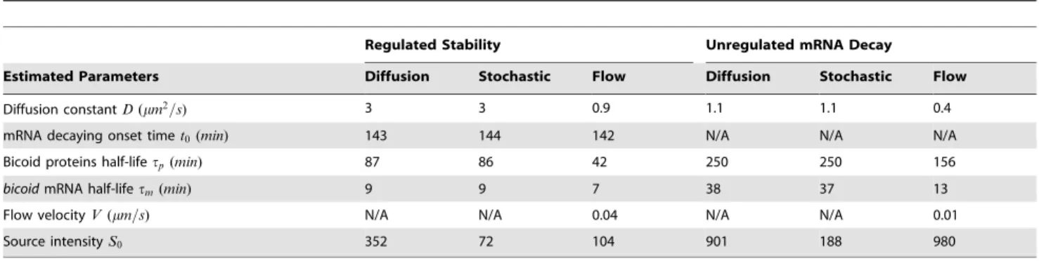
Values of estimated parameters for the different models are shown in Table 1, for the regulated stability model and a model in which source mRNA is permitted to decay from time zero (unregulated). We note that parameter values estimated by the fitting procedure are in sensible ranges used by previous authors. As already seen in Figure 1, for the regulated stability estimates, there is strong agreement across the three different models with respect to the onset of source decay (t0), and the speed at which it is decayed (tm), the main focus of our investigation. As noted in the Introduction, these observations confirm the experimental findings in [36] and [27]. Surdej and Jacobs-Lorena [36] argue that the mRNA is developmentally regulated,i.e.being held stable for up Figure 1. Spatio-temporal profiles of Bicoid and regulated anterior mRNA profiles inferred using three different computational models.(A)&(B) spatio-temporal profiles for a conventional model that assumes a constant source (drawn over two timescales). Inferred source profiles are in shown in (D), for deterministic diffusion (blue), cytoplasmic flow (red) and the stochastic (green) models. They differ in the source amplitudes required to fit the data, but the estimated decay onset times are very close. The corresponding spatio-temporal profile is shown in (C) over the full time and space axes. (E) and (F): model output and FlyEx data in the space-time range over which optimization was carried out. Profile shown in (E) is only for the deterministic diffusion model for clarity.

to the first two hours and then rapidly killed off in the next30 min. Spirovet al.[27] also suggest that the rapid degradation takes place over a15{20 mininterval. The rapid decay of mRNA suggested in both these papers is consistent with half-lives of 9, 9 and 7minutes inferred from our models.

We note that the diffusion constant estimated for Hechtet al.

[20]’s cytoplasmic flow model is smaller than the other two. This is to be expected since the motivation of this model is to use cytoplasmic flow as an additional trafficking mechanism that offsets a low diffusion constant. The value we estimated for flow velocity (0:04mm=s) is close to what was used in [20] (0:08mm=s), who take this estimate from observed nuclear motions. They note a 20-fold large range of possible values for this parameter, and use an average value. It is encouraging that the parameter obtained by fitting to FlyEx happens to be quite close.

The rightmost three columns of Table 1, show the parameter estimation for an unregulated source which allows for mRNA decay from time zero. This possibility is a natural expectation we need to explore, since mRNA molecules are inherently unstable. In order to match the measurements in the post-peak region, it turns out that this model not only has to amplify the source (S0) to almost ten times of the other models but also has to retain the protein in the medium for much longer period (tp~250&156 min). These values of protein half life are significantly higher than what is thought to be the half lives of Bicoid proteins [5]. Further, the source amplitude being so high is inconsistent with the observation that Bicoid protein is often undetectable during the very early stages of development ([5,19]). Thus, it is reasonable to conclude that the source supply is regulated as suggested by Surdej et al., rather than either kept constant throughout or be subject to natural decay.

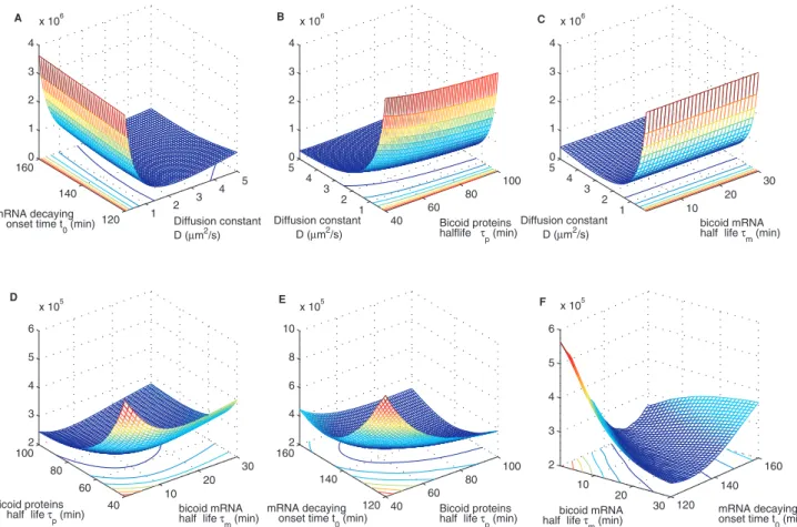
Figure 2 shows cross sections of the error function at the optimum point found by grid search. We have shown this with respect to all parameter combinations, taken pair-wise, setting the parameters not shown to their optimum values. The unimodal form of these error functions, shown here for the deterministic diffusion model, confirms that the optimization strategy we chose was adequate for this purpose. Similar error surface plots for the other two models are given in Figures S3, S4 and S5.

We note that previous authors working on Bicoid profiles have used a range of different values for diffusion and protein half-life parameters. For the diffusion constant, for example, values of,0:3 [13],7:0[41–43] and17mm2_{=sec[11,29] have been used. With} our models, we explored the effect of fixing one or more of the parameters at a value used by previous authors and optimizing the remaining parameters. We found the dominant effect is one of the

diffusion term compensating for the protein half-life, with the decay onset time and transcript half lives we compute showing far less variation.

We have further quantified the uncertainties in our estimates oft0 andtmby fitting the models to individual embryo measurements in FlyEx rather than their average profiles. We achieved this by constructing50reference datasets by uniformly bootstrapping from each temporal class in FlyEx. Figure 3 shows these uncertainties as box plots and confirms the fact that the estimated onset and decay rates are consistent across all three models.

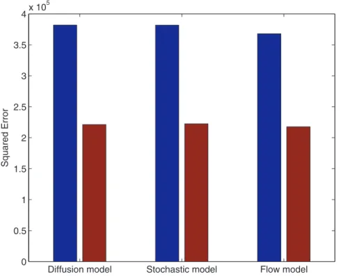
Figure 4 shows how the models achieve a reduction of almost a factor two, in the mean squared error between model outputs and FlyEx measurements in the post-peak region of nuclear cleavage cycles11{14A. This comparison between modelling errors, with and without our regulated source, confirms the merits of explicitly modelling the destruction of maternally deposited mRNA.

Our models permit the exploration of other published hypotheses about potential mRNA regulation. For example, Salles

et al.[40], treating the poly(A) tail length ofbicoidmRNA as proxy for its translational competence, suggest that protein production may be restricted in time, peaking between 1 to 1:5hours in development. We have simulated this by implementing the source as a rectangular function between 60 min and cycle 14A, and computing the resulting Bicoid profile (included as Figure S6). We found the corresponding modelling error to be significantly higher, caused mainly by forcing the decay to be instantaneous. While other, similar, explorations are possible with our approach (e.g. polysomal translation and translational bursting [44]), we believe the coarse nature of available data would mean one may have to be cautious about applying models of greater sophistication.

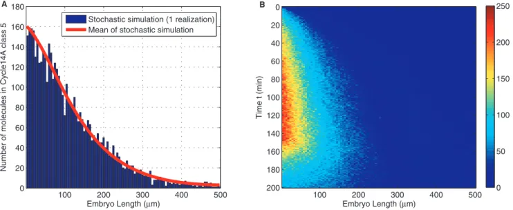
The results for Bicoid stochastic reaction diffusion in one run of stochastic simulation based on Gillespie algorithm Direct Method

(Algorithm 1) is shown in Figure 5. This model provides a more detailed understanding of the protein distribution, partitioned in compartments along A-P axis. We note that such a stochastic model characterizes a detailed view arising from molecular level variabilities. Our implementation in deriving the main results for the stochastic model in Table 1, following the technique of Erban

et al. [45], via simultaneous ordinary differential equations corresponding to discrete bins along the spatial axis (see Materials and Methods), captures average behaviour. Asymptotically (i.e.

with increasing number of bins), this is the equivalent of averaging a large number of Gillespie simulations, and should also give the same solution as the deterministic differential equation. To estimate the effect of molecular level variation, we matched

Flow velocityV(mm=s) N/A N/A 0.04 N/A N/A 0.01

Source intensityS0 352 72 104 901 188 980

Parameter values estimated by matching model outputs to observed data from FlyEx. Least squares fitting of model outputs to FlyEx with exhaustive search for the best combination of parameters on a regular grid suggests sensible values for the mRNA decay onset time,t0, in all three models. Regulated stability corresponds to an optimized period in time during which the mRNA is held stable and translated at a constant rate, followed by rapid decay. Unregulated stability is where the mRNA is allowed to decay from the very beginning; these parameters were estimated by forcingt0~0:01sin the optimization loop.

profiles generated by individual Gillespie simulations to bootstrap samples of Bicoid profiles from FlyEx (the same data used to derive uncertainties in Figure 3). As this process is computationally

demanding, we restricted ourselves to estimating the variability in mRNA decay onset time only, with the remaining parameters fixed to their optimal values given in Table 1. Matching such Figure 2. Cross sections through the error function between model output and measurements.Figures show the error function with respect to parameters taken pairwise, with those not shown held constant at their optimum values given in Table 1. Over the parameter ranges considered for the search, the error surface turns out to be unimodal for all three models. Deterministic diffusion model is shown above. Also see Figures S3, S4, S5 for other models considered.

doi:10.1371/journal.pone.0024896.g002

Figure 3. Uncertainty estimation.Uncertainty estimates of mRNA decay onset timet0in (A) and degradation timetmin (B) by fitting the models

individual simulations to data resulted in an increase in the standard deviation of estimation from3:9 minto5:5 min. While this increase suggests the variability at the molecular level may be captured by stochastic simulations, as in the study of Wuet al., the resulting estimation uncertainties in both cases are still small for the mRNA decay onset.

Spatially DistributedbicoidmRNA

While nearly all modelling work on Bicoid assume a spatial point source forbicoidmRNA, as noted earlier, Spirovet al.[27] suggest that thebicoidmRNA may have spatial distribution which alone explains the morphogen gradient at the protein level. They argue for an active transport mechanism along a cortical microtubular network. This proposal is questioned by Littleet al.

[41] who show experimental evidence that a distributed spatial gradient of mRNA is not sufficient to achieve the required morphogen profile. Since computational modelling of active transport hypothesized by Spirov et al.[27] is outside the scope of this study, we instead follow Dila˜o et al. [46] who have postulated an mRNA diffusion model to achieve an effect similar to that of Spirovet al.[27] (see Materials and Methods).

Figure 6 shows protein intensities with a spatial distribution for

bicoid mRNA. Figure 6A is profile obtained with only spatially distributed mRNA, while Figure 6B is results obtained with spatial distribution and temporal regulation and the post peak decay is clearly observed. Thus, even with simulated spatial distribution of maternal mRNA, our model finds a set of feasible parameter values that account for observed profiles in FlyEx. The corresponding parameter estimates are shown in Table S2. We find that the differences are in directions we would naturally expect:i.e.a spatially distributed maternal mRNA is compensated primarily by faster protein degradation. But it is encouraging to see that the onset of decay (t0) changes only slightly.

Materials and Methods

Deterministic Diffusion and Flow Model

The reaction diffusion equation used to model morphogen establishment is given by:

L

L_tM(x,t)~D L2

L_x2M(x,t){t

{1

p M(x,t)zS(x,t), ð1Þ where, M(x,t) is the morphogen concentration as a spatio-temporal function,D, the diffusion constant,tp, the half-life of the morphogen protein andS(x,t), the source at the anterior pole of embryo.

The flow model with one dimension fluid velocityVis defined by:

L

L_tM(x,t)~D L2

L_x2M(x,t){t

{1 p M(x,t)

{V L

L_xM(x,t)zS(x,t):

ð2Þ

In the original formulation of this model, the flow term was permitted to be active only for a short duration in time: nuclear cleavage cycles4to6depending on the motion of the nuclei in the viscous cytoplasm. In our implementation, we allowed this term to be present throughout the developmental time period considered, to increase its difference from the standard diffusion model.

The usual assumption in solving these models is that the source is constant: Scon~S0d(x)H(t), where S0 is the production rate, d(x) is the Kronecker delta function and H_{(t) is Heaviside step} function. The source model we propose here, incorporating regulated mRNA stability is given by:

Figure 4. Reduction in squared error between model outputs and FlyEx measurements.In all three models, nearly a factor two reduction is achieved by the improved source whose parameters are optimized. Blue bars represent modelling errors for a constant source model and the red bars correspond to the regulated mRNA model.

Scon{dec~S0d(x)ðH(t){H(t{t0)Þ

zS0d(x)H(t{t0)exp {

t{t0 tm

: ð3Þ

We use numerical methods available in the MATLAB PDE solver pdepe to solve these reaction diffusion models.

Stochastic Simulation Model

Closely following Wu et al. [21] and Erban et al. [45], the stochastic Bicoid protein reaction diffusion system we implement-ed simulates 100 compartments along the A-P axis, each with

lengthh~5mm, which is approximately the average size of one nucleus.

The three chemical reactions involved in this description are:

Bcd1' d d

. . .' d d

Bcdi' d d

. . .' d d

BcdN, for i~1,2,. . .,N ð4Þ

Bcdi t{1

p

6

O, for i~1,2,. . ._{,N ð5Þ}

6

O S(t) Bcdi, for i~1 ð6Þ Figure 5. One realization of stochastic simulation by Gillespie algorithm.Blue histogram, (A), shows the numbers of Bicoid molecules along anterior and posterior axis in embryo at a particular time point: cycle14Aclass5. Average of several such simulations is used as model output to match against measurements. (B) shows the realization jointly in space and time.

doi:10.1371/journal.pone.0024896.g005

Figure 6. The effect ofbicoidmRNA spatial gradient.(A) protein intensity without mRNA temporal regulation; (B) Bicoid profile with mRNA temporal regulation.

numbers to select the time at which a reaction occurs, and which one that is. The probability that j-th chemical reaction taking place is given by:aj=a0, where a0is a total propensity function, computed in step 2 (Algorithm 1).

Algorithm 1Bicoid reaction diffusion stochastic simulation.

Output:Vector of Bicoid molecular numbers,M

Initialization:M/0,t/0

whiletimevfinal timedo

1. Generate two random numbers which are uniformly distrib-uted in(0,1):r(1)andr(2).

2. Compute propensity functions for all of the reactions:

a0~a1za2za3za4.

3. Compute the time when next reaction occurs: tzt, where t~1=a0ln(1=r(1)).

4. Decide which reaction occurs at tzt: find j[R such that:

Xj{1

j~1aj=a0ƒr(2)v Xj

j~1aj=a0.

5. Update numbers of reactants and products inj-th reaction and sett/tzt.

end while

With vectorM, containing the number of molecules along the

N~100bins, Equations (4)–(6), define a total of R~3N{1 reactions. The propensity functions for the reactions are:

Bcd1 d

. . . d _BcdN: _a1~X

N{1

i~1

dM(i) ð7Þ

Bcd1 d

. . . d _BcdN : _a2~X

N

i~2

dM(i) ð8Þ

Bcdi t{1

p

6

O: _a3~X

N

i~1 t{1

p M(i) ð9Þ

In order to estimate parameters used in the stochastic model, Gillespie realizations are averaged. Erbanet al.derive the following system of ODEs for the different compartments to extract the ensemble average directly (see [45] for details):

L

L_tM1

~

(

{

)

{

{1

p M1zS(

t

,

L

LtMi~d(Miz1zMi{1{

2

)

{1

p Mi

,

by confocal scanning microscopy of fixed embryos, is the best available public domain dataset for this analysis. Measurements published in FlyEx are nuclear concentrations of Bicoid. The models we use, however, correspond to the total Bicoid. We make the assumption that the two concentrations are proportional across the developmental cycles. In recent work, Gregoret al.[13] have published some measurements of nuclear and cytoplasmic Bicoid concentrations, showing the dynamical balance between the two during cycles of nuclear division. Their data is suggestive that the use of nuclear concentrations as proxy for total concentrations is reasonable. Once we assume the two are proportional, parameters we infer by matching model outputs and data are unaffected, as any discrepancy will be absorbed by the source amplitude termS0, computed by Equation 15.

The spatio-temporal data for Bicoid we use, spans100points uniformly spaced along the A-P axis, and covers11points in time. The temporal range of measurements starts from nuclear cleavage cycle11to the end of cycle14A. Cycle14Ais of specific interest, because it is during this period, cellularization sets in and the established Bicoid profile begins to decay due to the decayingbicoid

mRNA. While there is some variability in how these develop-mental stages map onto real time, on average, cycle14A(temporal classes1{8) lasts for around50 min[47]. Cycle11starts around 100 minfrom fertilization, and the three cycles11, 12 and 13last an average of10 mineach. In FlyEx, Bicoid data is available for the11temporal classes from cycle11to14A.

The squared error between model output and measured intensities is

E~X

T₂

t~T₁ XL

x~1

S0M xð ,tÞ{Mdðx,tÞ

f g2, ð13Þ

h~arg min

h[H(E(h)), ð14Þ

where M(x,t) is the model output while Md(x,t) denotes the measured intensities from FlyEx.T1andT2are the boundaries of cleavage cycle11{14A.hin Equation (14) represents a vector of all unknown model parameters andH_{is the space over which we} search for optimum values.

Because the model output is linear in the source amplitudeS0 and is independent of the other parameters used in the three models, we calculate it in closed form rather than searching for an optimum in a grid. In order to minimise errorEin Equation (13), we differentiate it with respect toS0and equate it to zero. Then we haveS0as following:

S0~ XT₂

t~T₁ XL

x~1M(x,t)Md(x,t) XT₂

t~T₁ XL

x~1M(x,t)

bicoidmRNA Spatial Distribution

For mRNA spatial distribution, we follow Dila˜oet al.’s work in [46], but do not incorporate a term for natural mRNA decay. Thus instead of a diffusion equation, we restrict ourselves to the heat equation given by:

L_R

L_t ~Dr L2_R

L_x2, ð16Þ

whereDris mRNA diffusion constant. This is justified because our model for the temporal regulation ofbicoidmRNA is one which holds it stable up tot0followed by an active degradation.

Supporting Information

Figure S1 Spatio-temporal intensity profiles of

mor-phogen concentrations in four different models. (Ai),

solution to deterministic differential equation driven by a constant source (Aii); (Bi), (Ci) and (Di), solutions to deterministic diffusion, stochastic and cytoplasmic flow models, driven by the new source model incorporating regulated mRNA stability, and whose parameters are optimized.

(EPS)

Figure S2 Spatio-temporal profiles of model outputs and FlyEx data in the regions where model outputs were

matched to measured data (nuclear cleavage cycles11to

14A.(A), deterministic model driven by a constant source; Models driven by regulated source (C), (D) and (E), are deterministic diffusion, stochastic and cytoplasmic flow respectively. When mRNA regulation is included, all three models faithfully reproduce the temporal decay of the morphogen in the post-peak region. (EPS)

Figure S3 Modelling error displayed as functions of parameters taken pairwise. Stochastic simulation model.

(EPS)

Figure S4 Modelling error displayed as functions of parameters taken pairwise: Cytoplasmic flow model.

(EPS)

Figure S5 Modelling error surface for the cytoplasmic flow model as functions of flow velocity parameter and each of the other parameters.

(EPS)

Figure S6 Spatio temporal Bicoid profiles with source regulation as a step function, with constant rate of

translation between 60 min and onset of cycle 14A

(implementing[40]).

(EPS)

Table S1 Parameter optimization on a regular grid.

Table S1 shows the search spaces used in optimising the parameters of the three models considered. We used a coarse grid in the first round to get a rough estimate of the sensible range of parameters and followed it with a second round of search with a higher resolution and a reduced search range. Such a strategy is feasible, given we have only five parameters to estimate. Further, given the noisy nature of available data, searching over a finer grid to optimize parameters to a higher level of numerical precision does not make sense. If data of higher quality becomes available in the future, a scheme based on simulated annealing or population based optimisation needs to be considered. With the grid sizes we chose, shown in Table S1, it was possible to do least squares fitting of all three models on a desktop PC, with at most three days of wall clock time.

(PDF)

Table S2 Parameter estimation for stochastic model withbicoid_{mRNA regulation and spatial distribution.}

(PDF)

Acknowledgments

We thank Srinandan Dasmahapatra, Guido Sanguinetti and Martin Zeidler for helpful discussions during the course of this research. We also thank an anonymous reviewer for several insightful comments.

Author Contributions

Conceived and designed the experiments: WL MN. Performed the experiments: WL MN. Analyzed the data: WL MN. Contributed reagents/materials/analysis tools: WL MN. Wrote the paper: WL MN.

References

1. Turing AM (1952) The chemical basis of morphogenesis. Philosophical Transactions of the Royal Society of London Series B, Biological Sciences 237: 37–72.

2. Wolpert L (1969) Positional information and the spatial pattern of cellular differentiation. Journal of Theoretical Biology 25: 1–47.

3. Crick F (1970) Diffusion in embryogenesis. Nature 225: 420–422.

4. Driever W, Nu¨sslein-Volhard C (1988) The bicoid protein determines position in the Drosophila embryo in a concentration-dependent manner. Cell 54: 95–104. 5. Driever W, Nu¨sslein-Volhard C (1988) A gradient of bicoid protein in

Drosophila embryos. Cell 54: 83–93.

6. St Johnston D, Driever W, Berleth T, Richstein S, Nu¨sslein-Volhard C (1989) Multiple steps in the localization of bicoid RNA to the anterior pole of the Drosophila oocyte. Development 107: 13–19.

7. Driever W, Nu¨sslein-Volhard C (1989) The bicoid protein is a positive regulator of hunchback transcription in the early Drosophila embryo. Nature 337: 138–143.

8. Struhl G, Struhl K, Macdonald PM (1989) The gradient morphogen bicoid is a concentrationdependent transcriptional activator. Cell 57: 1259–1273. 9. Ephrussi A, Johnston DS (2004) Seeing is believing: The Bicoid morphogen

gradient matures. Cell 116: 143–152.

10. Houchmandzadeh B, Wieschaus E, Leibler S (2002) Establishment of developmental precision and proportions in the early Drosophila embryo. Nature 415: 798–802.

11. Gregor T, Bialek W, de Ruyter van Steveninck RR, Tank DW, Wieschaus EF (2005) Diffusion and scaling during early embryonic pattern formation. Proceedings of the National Academy of Sciences USA 102: 18403–18407. 12. Gregor T, Tank DW, Wieschaus EF, Bialek W (2007) Probing the limits to

positional information. Cell 130: 153–164.

13. Gregor T, Wieschaus EF, McGregor AP, Bialek W, Tank DW (2007) Stability and nuclear dynamics of the Bicoid morphogen gradient. Cell 130: 141–152.

14. Holloway DM, Harrison LG, Kosman D, Vanario-Alonso CE, Spirov AV (2006) Analysis of pattern precision shows that Drosophila segmentation develops substantial independence from gradients of maternal gene products. Developmental Dynamics 235: 2949–2960.

15. Porcher A, Dostatni N (2010) The Bicoid morphogen system. Current Biology 20: R249–R254.

16. Lo¨hr U, Chung HR, Beller M, Ja¨ckle H (2010) Bicoid - morphogen function revisited. Fly 4: 236–240.

17. Okabe-Oho Y, Murakami H, Oho S, Sasai M (2009) Stable, precise, and reproducible patterning of Bicoid and Hunchback molecules in the early Drosophila embryo. PLoS Computational Biology 5: e1000486.

18. He F, Saunders TE, Wen Y, Cheung D, Jiao R, et al. (2010) Shaping a morphogen gradient for positional precision. Biophysical Journal 99: 697–707. 19. Grimm O, Coppey M, Wieschaus E (2010) Modelling the Bicoid gradient.

Development 137: 2253–2264.

20. Hecht I, Rappel WJ, Levine H (2009) Determining the scale of the Bicoid morphogen gradient. Proceedings of the National Academy of Sciences USA 106: 1710–1715.

21. Wu YF, Myasnikova E, Reinitz J (2007) Master equation simulation analysis of immunostained Bicoid morphogen gradient. BMC Systems Biology 1: 52. 22. Gillespie DT (1977) Exact stochastic simulation of coupled chemical reactions.

The Journal of Physical Chemistry 81: 2340–2361.

2741–2749.

29. Bergmann S, Sandler O, Sberro H, Shnider S, Schejter E, et al. (2007) Pre-steady-state decoding of the Bicoid morphogen gradient. PLoS Biology 5: 965–991.

30. Reinitz J, Sharp DH (1995) Mechanism of eve stripe formation. Mechanisms of Development 49: 133–158.

31. Jaeger J, Surkova S, Blagov M, Janssens H, Kosman D, et al. (2004) Dynamic control of positional information in the early Drosophila embryo. Nature 430: 368–371.

32. Manu, Surkova S, Spirov AV, Gursky VV, Janssens H, et al. (2009) Canalization of gene expression and domain shifts in the Drosophila blastoderm by dynamical attractors. PLoS Computational Biology 5: e1000303.

33. Manu, Surkova S, Spirov AV, Gursky VV, Janssens H, et al. (2009) Canalization of gene expression in the Drosophila blastoderm by gap gene cross regulation. PLoS Biology 7: e1000049.

34. Ashyraliyev M, Siggens K, Janssens H, Blom J, Akam M, et al. (2009) Gene circuit analysis of the terminal gap gene huckebein. PLoS Computational Biology 5: e1000548.

35. Fomekong-Nanfack Y, Kaandorp JA, Blom J (2007) Efficient parameter estimation for spatiotemporal models of pattern formation: case study of Drosophila melanogaster. Bioinformatics 23: 3356–3363.

41. Little SC, Tkacˇik G, Kneeland TB, Wieschaus EF, Gregor T (2011) The formation of the Bicoid morphogen gradient requires protein movement from anteriorly localized mRNA. PLoS Biology 9: e1000596.

42. Abu-Arish A, Porcher A, Czerwonka A, Dostani N, Fradin C (2010) High mobility of Bicoid captured by fluorescence correlation spectroscopy: implication for the rapid establishment of its gradient. Biophysical Journal 99: L33–L35. 43. Porcher A, Abu-Arish A, Huart S, Roelens B, Fradin C, et al. (2010) The time to

measure positional information: maternal Hunchback is required for the synchrony of the Bicoid transcriptional response at the onset of zygotic transcription. Development 137: 2795–2804.

44. Kaern M, Elston TC, Blake WJ, Collins JJ (2005) Stochasticity in gene expression: from theories to phenotypes. Nature Reviews Genetics 6: 451464. 45. Erban R, Chapman SJ, Maini PK (2007) A practical guide to stochastic

simulations of reactiondiffusion processes. Arxiv preprint arXiv: 07041908. 46. Dila˜o R, Muraro D (2010) mRNA diffusion explains protein gradients in

Drosophila early development. Journal of Theoretical Biology 264: 847–853. 47. Foe VE, Alberts BM (1983) Studies of nuclear and cytoplasmic behaviour during