How to use MATLAB to fit the ex-Gaussian and other probability functions to a distribution of response times

2008, Vol. 4 (1), p. 35‐45. 

How

 

to

 

use

 

MATLAB

 

to

 

fit

 

the

 

ex

‐

Gaussian

 

and

 

other

 

probability

 

functions

 

to

 

a

 

distribution

 

of

 

response

 

times

 

Yves Lacouture  Université Laval   

Denis Cousineau  Université de Montréal 

 

This

 

article

 

discusses

 

how

 

to

 

characterize

 

response

 

time

 

(RT)

 

frequency

 

distributions

 

in

 

terms

 

of

 

probability

 

functions

 

and

 

how

 

to

 

implement

 

the

 

necessary

 

analysis

 

tools

 

using

 

MATLAB.

 

The

 

first

 

part

 

of

 

the

 

paper

 

discusses

 

the

 

general

 

principles

 

of

 

maximum

 

likelihood

 

estimation.

 

A

 

detailed

 

implementation

 

that

 

allows

 

fitting

 

the

 

popular

 

ex

‐

Gaussian

 

function

 

is

 

then

 

presented

 

followed

 

by

 

the

 

results

 

of

 

a

 

Monte

 

Carlo

 

study

 

that

 

shows

 

the

 

validity

 

of

 

the

 

proposed

 

approach.

 

Although

 

the

 

main

 

focus

 

is

 

the

 

ex

‐

Gaussian

 

function,

 

the

 

general

 

procedure

 

described

 

here

 

can

 

be

 

used

 

to

 

estimate

 

best

 

fitting

 

parameters

 

of

 

various

 

probability

 

functions.

 

The

 

proposed

 

computational

 

tools,

 

written

 

in

 

MATLAB

 

source

 

code,

 

are

 

available

 

through

 

the

 

Internet.

 

  In recent years there has been an upsurge of interest in  the response times (RT) of cognitive processes. This can be  attributed in  part to  the wide  availability  of computer  programs  that  allow  experiments  to  be  conducted  automatically and  RT  to  be measured  with  millisecond  precision. However, and perhaps more importantly, many  researchers see RT as major constraints when testing models  of  cognitive  processes.  Although  RT  are now routinely  measured  and  frequently  reported,  there  is  a  lack  of  standard  tools  for  characterizing  RT  distributions.  The  difficulty is that simple descriptive statistics usually do not  provide an adequate characterization of the data, and a 

             

  Address  correspondence  to:  Yves  Lacouture,  École  de 

Psychologie, Université Laval, Quebec City, Quebec, Canada  

G1K 7P4. Email: yves.lacouture@psy.ulaval.ca 

This work was supported by research and equipment grants  from  the  Natural  Sciences  and  Engineering  Research  Council of Canada (NSERC) to both authors. We would like  to thank Gene Bourgeau for his assistance in revising the  article. 

description in terms of probabilistic functions is generally  more suitable.  

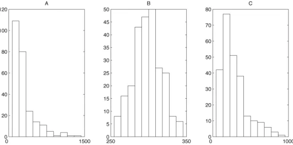
Figure 1. Three distributions of response times sampled from different populations each characterized by a specific probability functions. Panel (A) shows a distribution of response times shaped like an exponential function. Panel (B) shows data following a normal distribution and Panel (C) presents a distribution of data matching the ex‐Gaussian function. All  three distributions have the same mean x=300. 

6). A normal distributions of response times is typical of a  large variety of human performances including perceptual  and motor processes. Finally, distributions of response times  that follow the ex‐Gaussian function results of two or more  sequential processes made of a mixture of exponential and  normal  distributions.  Characterizing  the  shape  of  a  distribution of responses times allows a better description of  the results but also permits testing hypothesis about the  underlying cognitive processes.  

Finding  the  best  matching  distribution  to  a  set  of  response times provides information about the underlying  processes, but also the specific parameter values of the best  fitting function allows to test specific hypothesis. There are a  large number of probabilistic functions that can be used to  characterize  a  set of  response  times.  The  use  of  some  functions is  theoretically justified.  Other  functions yield  parameter  values  easier  to  interpret.  Among  the  wide  variety of functions that can be fitted to characterized a  distribution of response times, the ex‐Gaussian function is  especially popular because it is theoretically justified and  also because it provides parameter values that are easy to  interpret. For that reason, the ex‐Gaussian is the main focus  of this paper. 

Several researchers have shown that distribution analysis 

allows finding results that are not revealed by usual statistics.  Among  them,  Heahtcote,  Popiel  &  Mewhort  (1991)  presented data from the Stroop Task for which an analysis  of  mean  RT  misleadingly  showed  interference  but  no  facilitation whereas a distribution analysis showed both  interference  and  facilitation.  Other  studies  have  demonstrated  that some models that adequately  predict 

mean RT sometimes inadequately account for the shape of  RT  distributions  (Hockley  &  Corballis,  1982;  Ratcliff  &  Murdock, 1976). Also with distribution analyses, it was  shown that some visual searches proceed both in serial and  in parallel, whereas usual statistics yield to conclude that  the search is sequential (Cousineau & Shiffrin, 2003). Some  authors have also demonstrated the need to take the shape  of  RT  distributions  into  account  when  comparing  the  adequacy of different theoretical propositions (Hacker, 1980;  Hockley, 1984; Ratcliff, 1978, 1979). 

This  article  discusses  how  to  characterize  RT  distributions  in  terms  of  probability  density  functions  (especially using the ex‐Gaussian) and how to implement  the necessary analysis tools using MATLAB. Several key  features make MATLAB a popular choice as a simulation  package and analysis tool. First, the software runs on a  variety of platforms, including Windows, Mac OS, LINUX  and UNIX. Second, software implementations developed for  one platform can easily be transposed to other platforms.  Also,  MATLAB  provides  a  sophisticated  computational  environment with a simple, yet powerful, programming  language, debugging tools, and a sophisticated graphical  interface.  Also,  and  not  the  least,  MATLAB  is  computationally very efficient. Finally, a large community  of scientists develops and shares tools for the MATLAB  system. 

methods is presented in Myung (2003). In this paper, we  present an implementation that allows fitting the popular  ex‐Gaussian function. The last section of the paper reports a  Monte Carlo study that shows the validity of the proposed  approach. Although the main focus of the present paper is  the ex‐Gaussian function, the general procedure described  here can be used to estimate best fitting parameters of  various probability functions. The proposed computational  tools are written in MATLAB source code. They can be  customized and run in any MATLAB environment and are  available  through  the  Internet  at 

http://www.psy.ulaval.ca/~yves/distrib.html. 

Fitting Probability Density Functions to a Distribution of  Response Times 

A  probability  density  function  (PDF)  represents  the  distribution of values for a random variable. The area under  the curve defined the density (or weight) of the function in a  specific range. The density of a function is very similar to a  probability. Characterizing a phenomenon in terms of PDF  is very useful as it allows to estimate the probability that the  process yields values in a specific range. Some phenomena  in psychology are well described by PDF. For instance, the  distribution of results for most standardized intelligence  tests follows a Gaussian (normal) function. With a known  mean  and  standard  deviation,  the  probability  that  the  results of an intelligence test are in a specific range of values  can easily be computed. For example, a test characterized by  a Gaussian distribution of results with a mean of 100 and a  standard deviation of 15 implies that 50% of the population  have results above the mean while an IQ above 145 (three  standard deviations above the mean) corresponds to a very  low probability. 

The task of finding the parameter values of a probability  function that best represents the distribution of empirical  data is sometimes trivial. This is true, for example, when  considering the Gaussian (normal) function. In this case, the 

algebraic mean and standard deviation of the data are the  most accurate estimates of the mean and standard deviation  of the best‐fitting Gaussian function. In other cases, the task  of getting good estimations of the parameter values is more  complex.  

With  non‐trivial  cases,  like  the popular  ex‐Gaussian  function, an iterative approach allows the parameter space  to be searched and the parameter values that best fit a  frequency distribution to be estimated. To do this, the fit of  the probability function to the data is evaluated using a  goodness of fit (or error) criterion. An efficient and powerful  fit criterion is the likelihood value (see Myung, 2003 for a  tutorial). Given a data set and a PDF with specific parameter  values, the likelihood criterion provides an indication of the  fit  between  the  data  and  the  function.  The  best‐fitting  parameter values are associated with the greatest likelihood.  This is why this statistical approach is known as maximum  likelihood estimation. Given a PDF f(x | θ ) with k parameters  θ

=

[

θ

₁

,

θ

₂

,

…

,

θ

k

]

  and  an  empirical  set  of  data  composed of N observations _xi, i = 1, …, N, the likelihood  function is 

 

(

)

(

1

X |

N i i

Lθ f x θ

)

=

=

∏

| ,  (1) 

where 

Π

is the product operator. For large data sets, the  computation of the likelihood value returns values close to  zero and may provoke underflow errors. This is why the log  of  the  likelihood  criterion  is  often  used  instead  of  the  likelihood criterion. The log transformation substitutes the  sum operator to the product operator, less likely to provoke  overflow  errors.  For  historical  reasons,  minimization  procedures were more widespread, so it became customary  to minimize minus the log‐likelihood instead of maximizing  the log‐likelihood. The minus log‐likelihood criterion is 

 

(

)

(

)

1

X ln |

N

i i

LogLθ f x θ

=

⎡ ⎤

= −

∑

_{⎣ ⎦}

| ,  (2) 

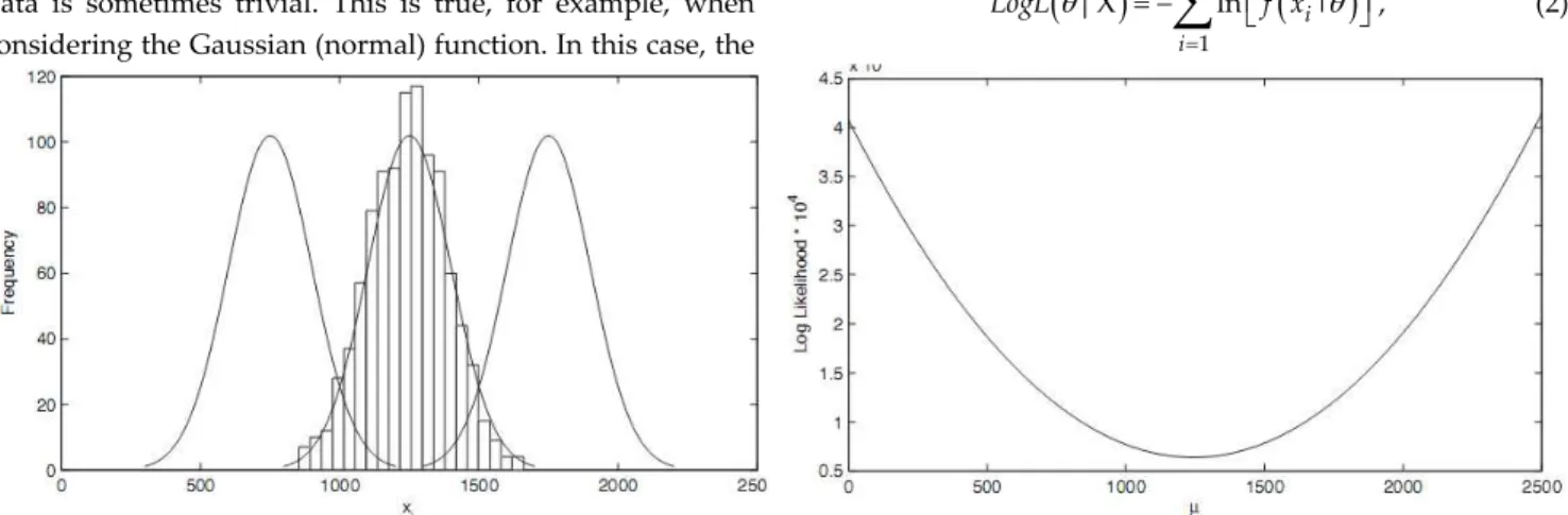
Figure 2. The minus log‐likelihood criterion for the Gaussian distribution computed for various value of parameter μ. The  left panel shows the correspondence between the frequency distribution and the PDF functions with parameters μ_A = 750, 

where  ln  is  the  natural  logarithmic  function.  Figure  2  illustrates how the LogL criterion is minimized when the  parameter  values  of  a  probability  function  best  fit  an  empirical distribution. The histogram (top panel) represents  a frequency distribution of N = 100 observations sampled  from a random variable that follows a Gaussian PDF with a  mean μ = 1250 and a standard deviation σ = 150. The top  panel also shows three overlay Gaussian PDFs (marked A,  B, and C), which have different mean values of μ_A = 750, 

μ_B = 1250, and μ_C = 1500. The three Gaussian PDFs have the 

same standard deviation σ = 150. Equation (2) allows LogL to  be computed according to the specific values of parameter μ.  For the Gaussian function, 

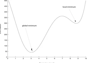
Figure 3. Global and local minima of a function: a search  algorithm  following  the  steepest  gradient  to  find  the  minimum of f(x|μ ) might get stuck in the local minimum  and converge without finding the global minimum. 

 

(

)

(

2

)

2 2

2

1

,

|

σ

μ

π

σ

σ

μ

− −

=

i i x

e

x

f

   and   

(

)

(

)

2

2

1 1

, | ln

2 2

i N

i

LogL X e

x μ σ σ π

μ

σ

= ⎡ ⎤ ⎢ ⎢ = − _⎢ ⎢ ⎢ ⎣ − −

∑

⎥⎥ ⎥ ⎥ ⎥ ⎦ .  (3) 

The  computation  yields  LogL(μA|X) = 11787, 

LogL(μB|X) = 6365, and LogL(μC | X) = 7835. It can be seen 

that LogL is smaller with parameter values that best fit the  frequency distribution. The bottom panel of Figure 2 shows  how, given the frequency distribution in the top panel, LogL  changes according to the value of parameter μ. LogL has a  minimum value for μ = 1250, which corresponds to the best‐ fitting Gaussian function. 

Searching Parameter Spaces With the Simplex Method 

To  find  the  parameter  values  that  correspond  to  a  minimum of the minus log‐likelihood criterion, a search of  the parameter space is required. Systematically trying all  possible values would certainly be time consuming. This is  especially true with functions that have several parameters  defining a multi‐dimensional space. Fortunately, there are  general purpose algorithms such as the Simplex method that  are  robust  and  allow  finding  a  minimum  of  a  multi‐ parameter  function  (see  Press,  Flannery,  Teukolsky  &  Vetterling,  1988,  for  a  review  of  search  methods  and  Cousineau, Brown and Heathcote, 2004 for a review in the  context of distribution analyses). Using the LogL criterion  with  the  Simplex  algorithm  allows  the  best‐fitting  parameters of a PDF to a distribution of data to be found  with great efficiency. 

The LogL criterion defines a fit  surface in a multi‐ parameter space. Starting with predetermined parameter  values, the Simplex method uses the steepest gradient on 

the  fit  surface  to  determine  how the  parameter  values  should  be  changed  to  improve  the  fit  of  the  adjusted  function. The algorithm follows an iterative procedure that  is applied until a minimum on the error surface is found.  The steepest gradient corresponds to the steepest slope on  the fit surface and, like a marble going down on a smooth  surface, allows a minimum of the function to be found. The  Simplex method works well providing that the fit surface is  continuous and smooth. This is generally the case when  using the LogL criterion with a reasonably large data set. 

Typically,  the  search  involves  changes  in  parameter  values that are made smaller at each iteration until the  adjustment yields only small changes in the fit criterion. The  search stops either when the improvement in fit is smaller  then  a  pre‐determined  criterion  or  when the change in  parameter values is smaller that another pre‐determined  value. The stopping criteria are called tolerances. The search  is said to have reached convergence when the improvement  in the goodness of fit is smaller than the termination tolerance  or when the change in parameter values is smaller than the  function tolerance.  

When the Search Fails to Converge: Local Minima and  Erratic Error Surfaces 

values. As mentioned before, this is usually not the case  when using the LogL criterion for which the error surface is  generally continuous and smooth. Second, it is possible that  the search gets stuck in a local minimum. A local minimum  is a region on the error surface that provides a minimum  that is not a global minimum of the function. Figure 3  illustrates  this  situation.  On  this  figure,  the  fit  surface  (vertical  axis)  is  a  function  of  a  single  parameter  θ  (horizontal axis). The function has a local minimum around  parameter value θ = 8.5 and a global minimum for θ = 3. In  this situation, like a marble rolling down the error surface,  the search algorithm might get stuck in the local minimum  and never reach the lower global minimum value. By doing  a few big steps on the fit surface in the beginning of the  search, most implementations of the Simplex method can  usually detect a local minimum and find a global minimum.  Nevertheless, a good strategy to avoid getting stuck in a  local minimum is to start the search process with parameter  values that are known to be in the neighborhood of the real  parameter  values.  For  example,  with  the  popular  ex‐ Gaussian  function,  a  reasonably  good  estimation  of  parameter μ is the difference between the algebraic mean  and the skewness of the data. Using this value as a starting  point for the search process reduces the risk of getting stuck  in a local minimum. Even with reasonable starting values,  the search may still fail to converge. When this happens,  three things can be done to increase the probability of  finding a global minimum of the function: (1) increase the  maximum  number  of  iterations  allowed  for  the  search  process, (2) perform a new search with different starting  parameter values, or (3) increase tolerances. 

Comparing the Fit of Different PDFs to the Same  Distribution of Data 

The LogL criterion does not allow the adequacies of  different probability functions that have different number of  parameters to be compared. For instance, the ex‐Gaussian  function has three parameters (μ, σ, τ), the Gaussian two  (μ, σ), and the Exponential function only one (τ). For a given  data set, the best‐fitting function is the one that yields the  smallest LogL value with the smallest number of parameters.  Hélie  (2006)  discusses  various  fit  criteria  that  allow  comparing the fit of functions (or models) having different  number of parameters. Among those fit criteria, Akaike’s  information criterion (AIC) is a popular goodness of fit  indicator that takes into account the number of parameters.  It is given by 

  AIC=2LogL

(

θ|X

)

+2k,  (4) 

where LogL is the minus log‐likelihood value and k is the  number of parameters of the fitted function. AIC is smaller  for probability functions with better fits. See Hélie (2006) for  more details. 

The ex‐Gaussian PDF 

The  ex‐Gaussian function  is the  convolution of  two  additive processes, a Gaussian (normal) function and an  exponential function. Luce (1986, chap. 6) describes the ex‐ Gaussian as a decision time model in cognitive processes.  Mathematically,  the  ex‐Gaussian  probability  density  function is written as 

 

2 2

2 1

( | , , ) exp 2

x x f x

σ μ

μ σ _τ

μ σ τ

τ τ τ τ σ

⎛ _{− −} ⎞

⎛ _{⎞ ⎜ ⎟}

⎜ ⎟

= _⎜ + − _{Φ⎜ ⎟}

⎟ ⎜ ⎟

⎝ _{⎠ ⎝ ⎠}

.  (5) 

In this equation, the exponential function (exp) is multiplied  by the value of the cumulative density of the Gaussian 

function  symbolized  by  Φ.  The  resulting  ex‐Gaussian  function has three parameters,  μ, σ, and τ. The two first  parameters (μ and σ) correspond to the mean and standard  deviation of the Gaussian component. The third parameter  (τ) is the mean of the exponential component. 

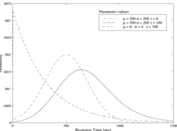
Figure 5. The ex-Gaussian PDF plotted for different parameter values.

In  the  framework  of  cognitive  processes,  this  convolution  can  be  seen  as  representing  the  overall  distribution of RT resulting from two additive or sequential  processes.  As  proposed  by  Luce  (1986,  chap.  6),  the  exponential process can be seen as the decision component,  i.e., the time required to decide which response to make,  while the Gaussian component can be conceptualized as the  transduction component, i.e., the sum of the time required by  the sensory process and the time required to physically  make the response. Although the theoretical proposition  that RT of cognitive processes are the sum of two additive  processes  is  difficult  to  test,  several  researchers  have  demonstrated that the ex‐Gaussian function provides a very  good fit to several empirical RT distributions (Ratcliff &  Murdock, 1976; Hockley, 1984; Luce,  1986). Other have  emphasized  that,  in  the  absence  of  any  theoretical  assumptions, the ex‐Gaussian function can effectively be  used to characterize an arbitrary RT distribution (Heathcote  et al., 1991). An interesting characteristic of the ex‐Gaussian  function  is  that  its  parameter  values  can  easily  be  interpreted. Parameters μ and σ are the mean and standard  deviation of the Gaussian component and can readily be  interpreted  as  localization  and  variability  indicators.  Parameter τ is the mean of the exponential component,  which corresponds to the right ‘tail’ of the distribution; a  larger τ implies a more skewed distribution. 

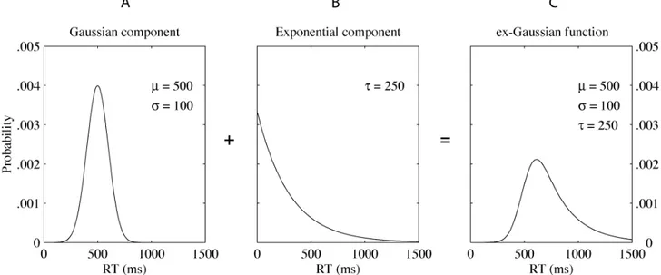
Figure 4 illustrates how an ex‐Gaussian function results  from two additive processes. If the time (in ms) required by  the normal process has a mean μ = 500 and a standard  deviation  σ = 100  (Panel  A  in  Figure  4),  and  the  time  required for completion of the second process follows an  exponential distribution with a mean τ = 250 (Panel B), then,  for a given trial, the resulting RT is the sum of a value  sampled from the Gaussian process and a value sampled  from the exponential process. The resulting distribution of  values follows the ex‐Gaussian probability function with  parameters μ = 500, σ = 100, and τ = 250 (Panel C) and has a  mean x= +μ τ and a standard deviation s= σ2+τ2 .  

Varying  the  parameters  of the  ex‐Gaussian  function  leads to a continuum of shapes from ‘pure’ exponential to  ‘pure’  Gaussian  functions.  Figure  5  presents  three  ex‐ Gaussian  curves  with  different  parameter  values.  As 

illustrated, with parameters μ = 0 and σ = 0, the ex‐Gaussian  function reduces to an exponential function. With parameter  τ = 0, the ex‐Gaussian function reduces to a normal function. 

One difficulty with the ex‐Gaussian function is that there  is  no  arithmetic  or  other  simple  way  to  derive  the  parameters of the underlying processes from the observable  data. To estimate the (unobservable) parameters, an iterative  procedure like the one discussed above is used to find the  parameter values for which the shape of the probability  function best fits the frequency distribution of data.  

Using MATLAB to Fit the Ex‐Gaussian Function to a  Frequency Distribution of RT 

This section presents a MATLAB implementation that  allows the popular ex‐Gaussian function to be fitted to a  frequency  distribution  of  data.  Implementing  a  search  algorithm  to  fit  the  ex‐Gaussian  PDF  to  an  empirical  distribution requires three MATLAB functions: 

1. A function implementing the ex‐Gaussian PDF;  2. A function implementing the computation of the 

LogL criterion for the ex‐Gaussian; 

3. A  search  algorithm  to  find  the  best‐fitting  parameter values. 

DISTRIB is a MATLAB toolbox comprising the necessary  functions to fit the ex‐Gaussian PDF. The complete set of  functions  is  presented  in  Appendix  1,  including  exgausspdf.m, which implements the ex‐Gaussian PDF. The  function takes the following form:  

Listing 1.the function simple_egfit 

func tion R=simple _e g fit(da ta )

ta u=std (d a ta ).*0.8; % re a so na b le sta rting va lue fo r ta u mu=me a n(d a ta )-ske wne ss(d a ta ); % re a so na b le sta rting va lue fo r mu sig =sq rt(va r(d a ta )-(ta u^2)); % re a so na b le sta rting va lue fo r sig

p init = [mu sig ta u]; % p ut sta rting p a ra me te r va lue s in a n a rra y % g ive n the d a ta , a nd p init, find the p a ra me te r % va lue s tha t minimize e g like

% the func tio n re turns R=[mu, sig , ta u] R=fminse a rc h(@ (p a ra ms) e g like (p a ra ms,d a ta ),p init);

 

Exgausspdf takes four arguments and returns the density  of the ex‐Gaussian PDFs with parameters mu, sigma, and tau,  given the value in data. Arguments mu, sigma (> 0), and tau  (> 0) are scalars (numbers) and argument data is either a  scalar, vector, or matrix. The function returns a vector of  probabilities f that has the same size as data. 

Function eglike.m returns the likelihood value computed  for the ex‐Gaussian PDFs given specific parameter values  and a data set. It has the following form: 

function logL=eglike(params, data). 

The  function  takes  two  arguments.  Argument  params = [mu, sigma, tau] is a three‐element vector that  specifies the parameter values of the ex‐Gaussian function.  The second argument is a vector of data for which the LogL  value is computed.   The function returns the minus log  likelihood for the ex‐Gaussian given the parameter values  and data. 

Function simple_egfit.m is a simple implementation that  performs parameter searches using the Simplex method.  This function is defined in Listing 1. 

Simple_egfit  takes  a  single  input  argument  data  (a 

column vector of data) and returns a three–element vector  R = [mu, sigma, tau] made of the best‐fitting ex‐Gaussian  parameter  values.  The  starting  values  for  the  search  procedure are estimated using simple heuristics. The search  is  done  using  MATLAB’s  fminsearch  function  that  implements the Simplex search method. Function eglike is  the fit criterion for the search process. Below is a description  of fminsearch, MATLAB’s implementation of the Simplex  method. 

Fminsearch_{, a MATLAB Function that Implements the} 

Simplex Method 

Fminsearch is a general purpose function that allows the  minimum of a multi‐parameter function to be found. To use  fminsearch with the LogL criterion, one needs to provide  fminsearch  with  (1)  the  name  of  the  function  to  be  minimized,  (2)  starting parameter values for  the  search  process, (3) the data to be fitted, and (4) some options that  control  the  tolerances  and  the  maximum  number  of  iterations in the search process. If no options are provided,  fminsearch  works  with  default  values.  The  format  of 

fminsearch is as follows: 

[x,fval,exitflag,output] = fminsearch(funfcn,x,options),  where funfcn is the function to be minimized, x is a vector  containing the  starting parameter values  for  the  search  process, options is another vector containing some options  that control the search process. Fminsearch returns a vector  containing  four  elements 

[x,fval,

 

exitflag,

 

output]. 

Element x contains the parameter values that correspond to  a minimum of the objective function; element fval  is the  value of the minimized function given the data and returned  parameters;  exitflag  and  output  provide  additional  information regarding the search process (for a detailed  description see MATALB’s Reference Guide). 

In simple_egfit, fminsearch is called as follows:  R=fminsearch(@(params) eglike(params, data),pinit) 

The string eglike(params,   data) indicates that function  eglike is to be minimized. Eglike return the likelihood for  the  ex‐Gaussian  function  given  the  parameters  in  params=[mu, sigma, tau] and the actual data. The first part  of the argument @(params) indicates which argument of  eglike is to be estimated, in that case, the parameters in  params while data is held constant. Also,  pinit is a vector 

containing the starting parameter values used when the  starting the search. In brief, the above syntax line calls  function fminsearch to find the parameters value (params)  for which function eglike show a minimum given the data.  The search is done starting with the parameter values in  pinit.  

Egfit.m, a More Robust Fitting Function for the Ex‐ Gaussian PDF 

Egfit is a MATLAB function that implements a more  flexible and robust search process to fit the ex‐Gaussian PDF  to a frequency distribution. This function has the following  form: 

function R = egfit(data, params, options).  

Egfit requires at least one argument data, which is a  vector containing the data for which the ex‐Gaussian is to be  fitted. Two optional arguments, params and options, allow  the search process to be controlled. Params = [mu, sigma,  tau] allows the starting parameter values for the search  process to be specified, and options = [ttolerance, ftolerance,  niter] allows optional controls for fminsearch to be set. The  optional tolerance values control the termination tolerance  (ttolerance) and the functional tolerance (ftolerance) 

of the Simplex method. Default values are 0.0001. Lastly,  optional argument niter controls the maximum number 

Table 1. Results  of  the  Monte  Carlo  study.  Mean  estimated parameters,  standard  errors,  and  confidence  intervals  for  each theoretical distribution and sample size 

ex-Gaussian

μ = 500 σ = 100 τ = 250

Sample Size

Mean Estimated Parameter (SD)

[95% interval]

10 _{μˆ = 536.1 (108.1)}

ˆ

σ = 76.2 ( 79.7)

ˆ

τ = 218.5 (125.2)

[377.2 - 845.5] [ 0.0 - 302.3] [ 20.2 - 457.4]

20 _μˆ = 514.3 (72.9)

ˆ

σ = 84.1 (60.7)

ˆ

τ = 241.7 (95.4)

[369.2 - 667.2] [ 0.0 - 210.3] [ 60.4 - 461.1]

30 _μˆ = 502.2 (54.1)

ˆ

σ = 88.4 (48.4)

ˆ

τ = 248.0 (76.3)

[405.7 - 590.0] [ 0.0 - 197.2] [119.4 - 405.7]

50 _μˆ = 488.6 (43.6)

ˆ

σ = 84.1 (35.7)

ˆ

τ = 258.3 (57.8)

[404.4 - 559.6] [ 0.0 - 140.8] [158.9 - 373.5]

100 _μˆ = 496.8 (26.6)

ˆ

σ = 96.4 (20.5)

ˆ

τ = 254.0 (39.7)

[449.8 - 552.0] [ 54.2 - 130.6] [165.7 - 317.0]

500 μˆ = 501.0 (12.2)

ˆ

σ = 99.7 ( 9.5)

ˆ

τ = 248.8 (15.8)

[476.2 - 526.6] [ 81.4 - 119.2] [218.2 - 279.7]

1000 μˆ = 500.6 ( 8.5)

ˆ

σ = 99.8 ( 6.5)

ˆ

τ = 249.3 (11.0)

[484.3 - 517.3] [ 87.0 - 112.5] [228.2 - 270.6]

5000 μˆ = 499.9 ( 3.9)

ˆ

σ = 100.0 ( 3.1)

ˆ

τ = 250.0 ( 4.9)

[492.5 - 507.6] [ 94.2 - 106.0] [240.5 - 259.2]

 

Table 1 (continued)

Ex-Gaussian

μ = 500 σ = 100 τ = 1000

Sample Size

Mean Estimated Parameter (SD)

[95% interval]

10 μˆ = 681.2 (285.8)

ˆ

σ = 113.3 (221.6)

ˆ

τ

= 856.5 (415.7)

[356.4 - 1492.2] [ 0.0 - 802.8] [ 86.6 - 1777.1]

20 μˆ = 566.5 (162.8)

ˆ

σ = 69.5 (134.2)

ˆ

τ = 967.2 (288.9)

[373.2 - 997.4] [ 0.0 - 460.2] [384.7 - 1571.8]

30 μˆ = 539.6 (124.8)

ˆ

σ = 75.3 (114.4)

ˆ

τ = 985.8 (245.0)

[368.4 - 901.2] [ 0.0 - 432.3] [559.8 - 1547.8]

50 _μˆ = 508.7 ( 76.8)

ˆ

σ = 71.9 ( 75.3)

ˆ

τ = 1012.2 (189.2)

[385.0 - 686.5] [ 0.0 - 231.5] [703.5 - 1489.6]

100 _μˆ = 498.3 ( 50.0)

ˆ

σ = 83.9 ( 50.4)

ˆ

τ = 1008.1 (122.5)

[409.8 - 619.2] [ 0.0 - 177.9] [798.4 - 1257.6]

500 μˆ = 500.2 ( 21.1)

ˆ

σ = 97.4 ( 16.9)

ˆ

τ = 1002.4 ( 50.5)

[461.0 - 542.4] [ 62.6 - 131.1] [907.7 - 1098.2]

1000 μˆ = 499.9 ( 13.7)

ˆ

σ = 98.7 ( 12.0)

ˆ

τ = 997.6 ( 33.4)

[474.1 - 528.3] [ 75.3 - 122.5] [934.8 - 1061.7]

5000 μˆ = 499.9 ( 6.7)

ˆ

σ = 99.1 ( 5.5)

ˆ

τ = 1000.7 (15.7)

[487.4 - 512.9] [ 89.3 - 109.9] [970.5 - 1032.6]

of iterations in the search process. The default value is  niter = 200*length(data). 

Testing egfit: a Monte Carlo Study 

A  Monte  Carlo  study  was  performed  to  evaluate  possible biases and estimate the standard error associated  with  the  parameter  estimates  when  using  the  present  implementation of the search process. The general approach  consisted of generating a large number of samples of fixed  size by  sampling  an  ex‐Gaussian random variable  with  known parameter values. Parameter estimations were then  obtained using egfit for each of the samples. This allowed 

a  distribution  of  estimated  parameter  values  to  be  reconstructed.  For  example,  consider  an  ex‐Gaussian  function with some specific parameters. By generating 1000  samples of size 100 and estimating the parameter values for  each  sample,  a  good  representation  of  the  sampling  distributions of the parameter values was obtained. The  standard  deviation  of  this  sampling  distribution  corresponds to the standard error for a given parameter and  sample  size.  Moreover,  the  mean  of  the  sampling  distribution can indicate possible biases. For an unbiased  estimator, the mean of the sampling distribution should be  close to the actual parameter value. A comprehensive and  detailed  Monte  Carlo  study  of  parameter  estimation  methods for popular probability functions is presented in  Van Zandt (2000). 

Method 

The Monte Carlo study was performed using two sets of  parameter values for the ex‐Gaussian function (EG1 and  EG2). For EG1, the parameter values were μ₁ = 500, σ₁ = 100,  and τ₁ = 250, and for EG2, they were  μ₂ = 500, σ₂ = 100, and  τ₂ = 1000.  

For each of the two theoretical distributions, the Monte 

Carlo study was performed for sample sizes N = 10, 20, 30,  50, 100, 500, 1000, and 5000. A Monte Carlo estimation of the  sampling distribution was obtained for each sample size by  sampling the theoretical distribution one thousand times  and performing a likelihood estimation of the parameters  for  each sample. Sixteen Monte  Carlo simulations (two  functions, EG1 and EG2 × 8 sample sizes), each based on  1000 samples, were performed. 

Results 

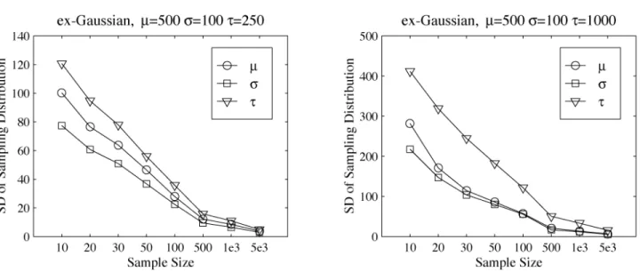
For each of the two theoretical functions, the sampling  distribution of each parameter was constructed for each  sample  size.  Table  1  summarizes  the  results.  For  each  sample  size,  the  mean  and  standard  deviation  of  the  sampling  distribution  are  presented  along  with  a  95 %  confidence interval based on the observed percentile values  of the distribution. Figure 6 shows the average estimated  parameter values plotted according to sample size for each  distribution.  

The sampling distributions show some small biases for  smaller sample sizes. For the specific parameter values used  in this  Monte Carlo  study, the  means  of the sampling  distributions do not appear strongly biased for sample sizes  of 100 or more. Figure 7 presents the standard deviations of  the  sampling  distributions  (the  standard  error)  plotted  according  to  sample  size.  For  both  of  the  ex‐Gaussian  distributions, the results show a monotonic decrease with an  increase in sample size. The decrease in standard deviation  with increasing sample size is sharp up to sample size N =  500. The Monte Carlo study shows that egfit provides good  parameter estimations for the ex‐Gaussian function, at least  for the test values that were used. 

Conclusion 

This paper discusses the problem of characterizing RT 

distributions in terms of probability functions. The functions  implemented in this paper provide simple and efficient  ways  to  estimate  parameter  values  of  the  ex‐Gaussian  function. A Monte‐Carlo study has shown the validity of the  proposed implementation. Other implementations can be  developed with the same approach using the MATLAB  fminsearch function, as discussed in the present paper. 

References 

Cousineau, D., Brown, S., & Heathcote, A. (2004). Fitting  distributions using maximum likelihood: Methods and  packages.  Behavior  Research  Methods,  Instruments,  &  Computers, 36, 742‐756. 

Cousineau, D., & Shiffrin, R. M. (2004). Termination of a  visual search with large display size effect. Spatial Vision,  17, 327‐352. 

Hacker,  M.  J.  (1980).  Speed  and  accuracy  of  recency  judgments for events in short‐term memory. Journal of  Experimental Psychology: Human Learning and Memory, 6,  651‐675. 

Heathcote, A., Popiel, A. J., & Mewhort, D. J. K. (1991).  Analysis  of  response time distributions: An  example  using the Stroop Task. Psychological Bulletin, 109, 340‐347.  Hélie, S. (2006). An introduction to model selections: Tools  and  algorithms.  Tutorials  in  Quantitative  Methods  for  Psychology, 2, 1‐10. 

Hockley,  W.  E.  (1984).  Analysis  of  response  time  distributions in the study of cognitive processes. Journal  of  Experimental  Psychology:  Learning,  Memory  and  Cognition, 6, 598‐615. 

Hockley, W. E. & Corballis, M. C. (1982). Test of serial  scanning  in  item  recognition.  Canadian  Journal  of  Psychology, 36, 189‐212. 

Luce,  R.  D.  (1986).  Response  times.  New  York:  Oxford  University Press. 

Myung,  I.J.  (2003).  Tutorial  on  maximum  likelihood  estimation. Journal of Mathematical Psychology. Vol 47(1),  90‐100. 

Press, W. H., Flannery, B. P., Teukolsky, S. A. & Vetterling,  W.  T.  (1988).  Numerical  recipes:  The  art  of  scientific  computing. Cambridge, England: Cambridge University  Press. 

Ratcliff,  R.  (1978).  A  theory  of  memory  retrieval.  Psychological Review, 85, 59‐108. 

Ratcliff, R. (1979). Group reaction time distributions and an  analysis of distribution statistics. Psychological Bulletin,  86, 446‐461. 

Ratcliff, R. & Murdock, B. B. (1976). Retrieval processes in  recognition memory. Psychological Review, 83, 190‐214.  Van Zandt, T. (2000). How to fit a reaction time distribution. 

Psychonomic Bulletin and Review, 7(3), 424‐465. 

Manuscript received February 23, 2007 

Appendix 

Description of the functions in DISTRIB, a MATLAB toolbox implementing the fitting process for the ex‐Gaussian  PDF 

a ic .m y = a ic (lo g l, k)

Given the minus log likelihood value logl and the number of parameters k, returns  Akaine’s information criterion. Both arguments must be the same size.  

simp le _e g fit.m R = simp le _e g fit(d a ta )

Simple  implementation of  the  search  process  to fit the  ex‐Gaussian function  using  MATLAB’s implementation of the Simplex search method. Argument data is a column  vector containing the data to be fitted. The function returns a maximum likelihood  estimate of parameter values for the data in hand.  

R = [mu, sig , ta u] c o nta ins the thre e e stima te d e x-Ga ussia n p a ra me te rs.

e g fit.m R = e g fit(d a ta )

R = e g fit(d a ta , p a ra ms, o p tio ns)

R = e g fit(d a ta , [mu, sig , ta u], [tto le ra nc e , fto le ra nc e , nite r])

Does a parameter search for the ex‐Gaussian function using MATLAB’s implementation of  the Simplex search method. This implementation is more robust and flexible than function  simple_egfit. Argument data is a column or row vector containing the data to be fitted.  Optional argument params = [mu, sig, tau] allows starting parameter values for the search  process to be specified; optional argument options = [ttolerance, ftolerance, niter] allows  optional controls for fminsearch to be set; The optional tolerances control the termination  tolerance (ttolerance) and the functional tolerance (ftolerance). Default tolerance is 0.0001.  Optional argument niter controls the maximum number of iterations in the search process.  The default value is niter = 200 * length(data).  

R = [mu, sig, tau] contains the three estimated ex‐Gaussian parameters. 

e g like .m lo g l = e g like (p a ra ms, d a ta )

Given parameters  params = [mu, sigma, tau] and vector data, returns  the  minus log‐ likelihood value for the ex‐Gaussian function. 

e xg a ussp d f.m f = e xg a ussp d f(mu, sig , ta u, x)

Returns the probability at value x of the density function for the ex‐Gaussian distribution  with parameters mu, sig, and tau. 

e xp p d f.m y = e xp p d f(x, mu)

Returns the probability at value x of the density function for the exponential distribution  with parameter mu. 

p lo te g fit.m p lo te g fit(p a ra ms, d a ta )

Plots  an histogram of  data  vector with overlay  ex‐Gaussian PDFs  with parameters  params = [mu, sigma, tau]. 

p nf.m p =p nf(x, mu, sig )

Returns the cumulative value, observed at x, for the density function of the Gaussian  distribution with parameters mu and sig.