DEPARTAMENTO DE ENGENHARIA DE TELEINFORMÁTICA
PROGRAMA DE PÓS-GRADUAÇÃO EM ENGENHARIA DE TELEINFORMÁTICA
IGOR MOACO GUERREIRO
DISTRIBUTED OPTIMIZATION TECHNIQUES FOR 4G AND BEYOND
DISTRIBUTED OPTIMIZATION TECHNIQUES FOR 4G AND BEYOND
Tese apresentada ao Curso de Doutorado em Engenharia de Teleinformática da Universidade Federal do Ceará, como parte dos requisitos para obtenção do Título de Doutor em Engenha-ria de Teleinformática. Área de concentração: Sinais e Sistemas
Orientador: Prof. Dr. Charles Casimiro Caval-cante
Gerada automaticamente pelo módulo Catalog, mediante os dados fornecidos pelo(a) autor(a)
G965d Guerreiro, Igor Moaco.
Distributed Optimization Techniques for 4G and Beyond / Igor Moaco Guerreiro. – 2016. 134 f. : il. color.
Tese (doutorado) – Universidade Federal do Ceará, Centro de Tecnologia, Programa de Pós-Graduação em Engenharia de Teleinformática, Fortaleza, 2016.
Orientação: Prof. Dr. Charles Casimiro Cavalcante.
1. Otimização distribuída. 2. Troca de mensagens. 3. Seleção de Precodificadores. 4. Descoberta de feixes. I. Título.
DISTRIBUTED OPTIMIZATION TECHNIQUES FOR 4G AND BEYOND
Tese apresentada ao Curso de Doutorado em Engenharia de Teleinformática da Universidade Federal do Ceará, como parte dos requisitos para obtenção do Título de Doutor em Engenha-ria de Teleinformática. Área de concentração: Sinais e Sistemas
Aprovada em: 30/06/2016.
BANCA EXAMINADORA
Prof. Dr. Charles Casimiro Cavalcante (Orientador) Universidade Federal do Ceará
Prof. Dr. André Lima Ferrer de Almeida Universidade Federal do Ceará
Prof. Dr. Tarcisio Ferreira Maciel Universidade Federal do Ceará
Prof. Dr. Marcello Luiz Rodrigues de Campos Universidade Federal do Rio de Janeiro
I am very thankful to people at GTEL, specially Prof. Charles Cavalcante for his great Ph.D. supervision. Thanks GTEL and the Innovation Centre, Ericsson Telecomunicações S/A, Brazil, for the financial support during the whole period of the Ph.D. course.
I am also very thankful to people at the RAT department at Ericsson Research, specially Dennis Hui for having introduced me to factor graphs and message-passing algorithms, and Johan Axnäs for his remarkable supervision during my Ph.D. internship from September-2014 until August-2015 in Kista, Sweden. I am also thankful to Prof. Mats Bengtsson, who was a contact person at KTH Royal Institute of Technology, Stockholm, during my Ph.D. internship, and to CAPES Foundation, Ministry of Education of Brazil, for the financial support.
Thanks for my family, specially my parents Manoel and Marlene, and my sister Lígia, for being always present with their priceless love. Also lots of thanks to all my friends for their sincere friendship.
In today’s and future wireless telecommunication systems, the use of multiple antenna elements on the transmitter side, and also on the receiver side, provides users a better experience in terms of data rate, coverage and energy efficiency. In the fourth generation of such systems, precoding emerged as a relevant problem to be optimally solved so that network capacity can be increased by exploiting the characteristics of the channel. In this case, transmitters are equipped with few antenna elements, say up to eight, which means there are a few tens of precoding matrices, assuming a discrete codebook, to be coordinated per transmitter. As the number of antenna elements increases at communication nodes, conditions to keep in providing good experience for users become challenging. That’s one of the challenges of the fifth generation. Every transmitter must deal with narrow beams when a massive number of antenna elements is adopted. The hard part, regarding the narrowness of beams, is to keep the spatial alignment between transmitter and receiver. Any misalignment makes the received signal quality drop significantly so that users no longer experience good coverage. In particular, to provide initial access to unsynchronized devices, transmitters need to find the best beams to send synchronization signals consuming as little power as possible without any knowledge on unsynchronized devices’ channel states. This thesis thus addresses both precoding and beam finding as parameter coordination problems. The goal is to provide methods to solve them in a distributed manner. For this purpose, two types of iterative algorithms are presented for both. The first and simplest method is the greedy solution in which each communication node in the network acts selfishly. The second method and the focus of this work is based on a message-passing algorithm, namely min-sum algorithm, in factor graphs. The precoding problem is modeled as a discrete optimization one whose discrete variables comprise precoding matrix indexes. As for beam finding, a beam sweep procedure is adopted and the total consumed power over the network is optimized. Numerical results show that the graph-based solution outperforms the baseline/greedy one in terms of the following performance metrics: a) system capacity for the precoding problem, and b) power consumption for the beam finding one. Although message-passing demands more signaling load and more iterations to converge compared to baseline method, it usually provides a near-optimal solution in a more efficient way than the centralized solution.
Nos sistemas de telecomunicações sem fio atuais e futuros, o uso de múltiplos elementos de antena no lado do transmissor, e também no do receptor, proporciona aos usuários uma melhor experiência em termos de taxa de dados, cobertura e eficiência energética. Na quarta geração de tais sistemas, precodificação surgiu como um problema relevante a ser solucionado de forma ótima de modo que a capacidade da rede pudesse ser aumentada explorando as características do canal. Neste caso, transmissores são equipados com alguns elementos de antena, por exem-plo, oito, o que resulta em algumas dezenas de matrizes de precodificação, assumindo um con-junto discreto, para serem coordenadas em cada transmissor. Com o crescimento no número de elementos de antena nos nós de comunicação, as condições para continuar provendo boa ex-periência para usuários se tornam desafiantes. Isto é um dos desafios da quinta geração. Cada transmissor deve lidar com feixes estreitos quando é adotado um número massivo de elemen-tos de antena. A parte complicada, considerando a pequena largura dos feixes, é a manutenção do alinhamento espacial entre transmissor e receptor. Qualquer desalinhamento desta natureza faz a qualidade do sinal recebido cair significativamente de tal forma que usuários deixam de perceber boa cobertura. Particularmente, para prover acesso inicial a dispositivos não sincroni-zados, transmissores necessitam achar os melhores feixes, sem nenhum conhecimento do estado de canal de tais dispositivos não sincronizados, para enviar sinais de sincronização consumindo o mínimo de energia possível. Esta tese, portanto, discute ambos os problemas de precodifica-ção e descoberta de feixes como sendo de coordenaprecodifica-ção de parâmetros. A meta é prover métodos para solucioná-los de maneira distribuída. Para este propósito, dois tipos de algoritmos iterativos são apresentados para ambos os problemas. O primeiro método, e o mais simples, é a solução “gulosa”, na qual cada nó de comunicação na rede atua de forma egoísta. O segundo método,
e o foco deste trabalho, é baseado em um algoritmo de troca de mensagens, especificamente o algoritmo min-sum, em grafos fatores. O problema de precodificação é modelado como um de otimização discreta onde as variáveis discretas compreendem índices de matrizes de precodifi-cação. A respeito da descoberta de feixes, é adotado um procedimento de varredura de feixes com a otimização do consumo total de potência na rede. Resultados numéricos mostram que a solução baseada em grafos ganha da egoísta, que é usada como solução base, em termos da mé-trica de desempenho: a) capacidade do sistema para o problema de precodificação, e b) consumo de potência para o caso de descoberta de feixes. Embora a troca de mensagens demande mais carga de sinalização e mais iterações para convergir comparado ao método base, ela geralmente provê uma solução próxima da ótima de forma mais eficiente comparada a solução centralizada.
Figure 1.1 – Example of setup for a given network that adopts (a) centralized solution and (b) distributed solution. In the former, every communication node has a link with a central unit, while in the latter each node is linked with just a few neighboring nodes. . . 19 Figure 2.1 – A general network example with a seven-cell hexagon layout. Each cell has a
communication node which shares the set of resources available in the network. 27 Figure 2.2 – An example of frequency reuse planning in a seven-cell hexagon layout. The
parameter vectorp = [1 3 2 3 2 3 2]T is one of the optimal solutions of the
problem, where Pi = {1,2,3} fori = 1,2, . . . ,7. That is, no collision is
observed among communication nodes. . . 29 Figure 2.3 – Estimated power coupling matrix Ωof 2x3 MIMO channel matrices. Only
the Tx. eigenmode 1 couples to the Rx. eigenmodes. . . 34 Figure 2.4 – Example of a factor graph model for a 7-cell communication network with
local parameters and local performance measures. . . 38 Figure 2.5 – Re-organized factor graph for a communication network with local
parame-ters and local performance measures. . . 38 Figure 2.6 – Fragment of a factor graph, showing the message pass between factor node
Mi and variable nodepk. . . 39
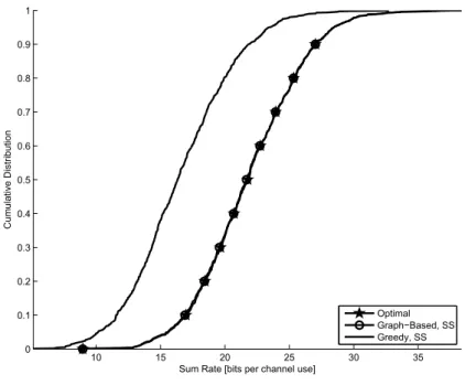
Figure 2.7 – Graphical model of the prisoner’s dilemma. Step 0 (i.e. the initial condition) of the graph-based algorithm as well as steps 1-4 for the first iteration are illustrated. . . 42 Figure 2.8 – Performance analysis of graph-based technique for TAS problem in terms of
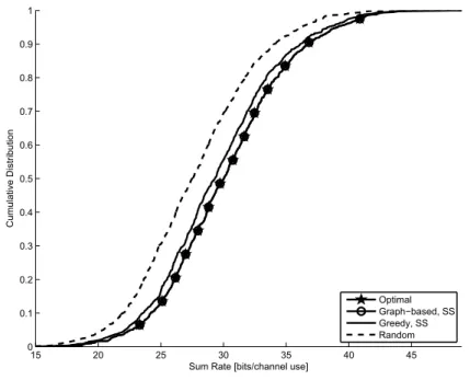
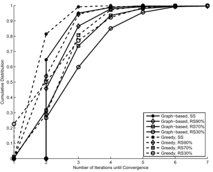
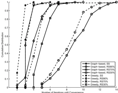
sum rate in 7-node network. . . 48 Figure 2.9 – Convergence speed of graph-based technique against greedy technique for
TAS problem in 7-node network. . . 49 Figure 2.10–Performance analysis of graph-based technique for TAS problem in terms of
sum rate in 61-node network. . . 50 Figure 2.11–Convergence speed of graph-based technique against greedy technique for
TAS problem in 61-node network. . . 51 Figure 2.12–Performance analysis of graph-based technique for beam selection problem
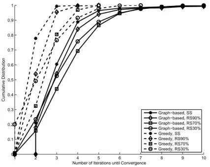
in terms of sum rate in 7-node network. . . 53 Figure 2.13–Convergence speed of graph-based technique against greedy technique for
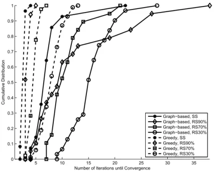
beam selection problem in 7-node network. . . 54 Figure 2.14–Performance analysis of graph-based technique for beam selection problem
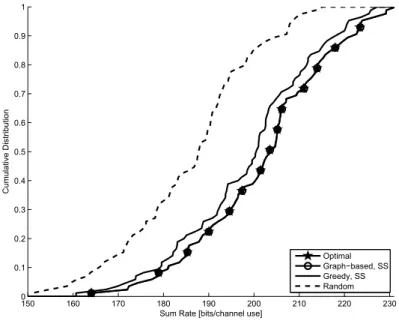
beam selection problem in 61-node network. . . 57 Figure 2.16–Performance analysis of graph-based technique for LTE codebook in terms
of sum rate in a 7-node network. . . 59 Figure 2.17–50-th CDF percentile of sum rate for LTE codebook in a 7-node network. . . 60 Figure 3.1 – Signaling load analysis showing the amount of information exchange per
node against the number of neighbors Nu and |P| = 3. For Nu > 3, a
centralized approach causes more signaling load. . . 65 Figure 3.2 – Performance analysis of graph-based technique for the precoder selection
problem in terms of system throughput in 19-node network. . . 68 Figure 3.3 – CDF percentile of system throughput per iteration in 19-node network. It
shows how much gain the graph-based technique obtains over the greedy. . 69 Figure 3.4 – Performance analysis of graph-based technique for the precoder selection
problem in terms of convergence speed in 19-node network. . . 70 Figure 4.1 – AN sends system information for initial synchronization using a narrow beam
to an arbitrary direction. Two unsynchronized UEs try to establish connec-tion, but only one is satisfactorily covered. . . 73 Figure 4.2 – Example of a mm-Wave indoor scenario. Orange crosses in the illustration
denote UE data samples collected by access nodes (ANs), which are eventu-ally treated as virtual UEs to emulate UEs in the optimization. . . 76 Figure 4.3 – Example of beam sweeping in a room with a single AN. The effective beam
shape after 13 beam sweep instances coincides with the relevant area. . . 77 Figure 4.4 – Examples of power consumption model function Ψm vs. Pm. On the right
side, Ψm(Pm) is a linear relation, while on the right it is based ona priori
information. Variable nodemknows the power levelsP¯m,k andP¯m,k′ to in-dividually satisfy virtual UEk and UEk′, respectively. . . 79
Figure 4.5 – Factor graph with check nodes, variable nodes and factor nodes. Curved rec-tangles delimit the local beams at ANs. Squares in gray denote check nodes, while squares in white denote factor nodes. . . 84 Figure 4.6 – Flowchart that illustrates all the steps of the MP algorithm. . . 86 Figure 4.7 – Check nodes inside an AN denote the emulation of the virtual UEs the
be-ams of that AN were heard by. In this example, the AN on the left emulates three virtual user equipments (UEs), while the one on the right emulates the remaining two virtual UEs. Note that the message exchange between beams of the same AN is performed locally, whereas the message exchange among beams of different ANs takes place over some backhaul. . . 89 Figure 4.8 – Total transmit power forPmaxset to20mW against iterations. . . 91
one UE per square meter and a single AN placed in the middle of the office. 94 Figure 4.11–Comparison among solutions provided by MILP, and both granular MP (with
80%MP scheduling) and baseline algorithms, for a scenario with two ANs,
16 beams per AN and 24 UEs. . . 95 Figure 4.12–Average total consumed power against check node degreeD for100%and
80% random scheduling and single AN. Note that the MP algorithm with 100%random scheduling converged a few times only forD= 3. . . 98
Figure 4.13–Average total consumed power against check node degree D for 60% and 20%random scheduling and single AN. . . 99
Figure 4.14–Convergence rate against check node degreeD for different random
schedu-ling percentages and single AN. . . 99 Figure 4.15–Average number of iterations until convergence against check node degree
D for different random scheduling percentages and single AN. . . 100
Figure 4.16–Average total consumed power against check node degreeD for100%and 80%random scheduling and two ANs. . . 103
Figure 4.17–Average total consumed power against check node degree D for 60% and 20%random scheduling and two ANs. . . 103
Figure 4.18–Convergence rate against check node degreeD for different random
schedu-ling percentages and two ANs. . . 104 Figure 4.19–Average number of iterations until convergence against check node degree
D for different random scheduling percentages and two ANs. . . 104
Figure 4.20–Average total consumed power against check node degreeD for100%and 80%random scheduling and four ANs. . . 107
Figure 4.21–Average total consumed power against check node degree D for 60% and 20%random scheduling and four ANs. . . 107
Figure 4.22–Convergence rate against check node degreeD for different random
schedu-ling percentages and four ANs. . . 108 Figure 4.23–Average number of iterations until convergence against check node degree
D for different random scheduling percentages and four ANs. . . 108
Figure 5.1 – Two types of beam sweep cycles: (a) optimized beam sweep, and (b) exhaus-tive beam sweep. In the latter, synchronization signals are transmitted over the whole service area of ANs, while in the former ANs follow an optimi-zed beam sweep parameter setting based on historical statistics of UEs. An exhaustive beam sweep cycle with durationtfullis repeated with periodTfull.
Sequences ofK optimized beam sweep cycles, each one with durationtopt,
signal by an unsynchronized UE. Upon reception of a synchronization signal, the UE detects and decodes the information conveyed by the signal. Then, it can synchronize in time and frequency. Additionally, it can calculate the corresponding per-beam received signal quality. It can also calculate the cor-responding scanning delay, i.e., the time elapsed between it started seeking for synchronization until the synchronization itself. The signal quality and the scanning delay are used to generate a time-stamped UE data sample to be fed back to the AN that sent the corresponding synchronization signal. . . 114 Figure 5.3 – Design example of a time-stamped UE data sample that comprises
informa-tion on transmit beam direcinforma-tion, receive beam direcinforma-tion, received synchroni-zation signal quality and scanning delay. . . 115 Figure 5.4 – Block diagram that generally illustrates the reception of some time-stamped
UE data samples from a synced UE. The information conveyed by the data reported by the synced UE is used by the AN that received such data samples to update some available set of historical statistics (UE dataset), as well as to check how long the reporter synced UE waited until it could synchronize. The scanning delaytscanis compared with a delay threshold given byτmax: if
τscan > τmax, it means that the reporter synced UE waited too long for
syn-chronization, then the optimized beam sweep parameters must be readjusted by running the beam sweep optimizer; otherwise, the AN keeps the same op-timized beam sweep parameter setting, meaning that the reported scanning delay is tolerable. . . 115 Figure 5.5 – Example of check node splitting. A fragment of a standard factor graph has
its check node splitρktimes. . . 117
Figure 5.6 – Example of factor graph showing check nodekand variable nodesmandνin
its neighborhood. To compute summary messageα(k→mt+1), check nodekfinds
Table 1 – List of neighboring communication nodes of network example in Figure 2.1. 28
Table 2 – Summary of the GRASS algorithm. . . 36
Table 3 – Graph-based distributed parameter coordination algorithm. . . 41
Table 4 – General simulation parameters. . . 46
Table 5 – Simulation parameters for TAS. . . 47
Table 6 – Percent gain in sum rate for the transmit antenna selection (TAS) problem in a 7-node network. . . 47
Table 7 – Convergence rate for TAS problem in 7-node network. . . 48
Table 8 – Percent gain in sum rate for TAS problem in 61-node network. . . 50
Table 9 – Convergence rate for TAS problem in 61-node network. . . 50
Table 10 – Simulation parameters for fixed-beam selection. . . 52
Table 11 – Percent gain in sum rate for beam selection problem in 7-node network. . . . 54
Table 12 – Convergence rate for beam selection problem in 7-node network. . . 54
Table 13 – Percent gain in sum rate for beam selection problem in 61-node network. . . 55
Table 14 – Convergence rate for beam selection problem in 61-node network. . . 56
Table 15 – Simulation parameters for LTE precoder selection. . . 58
Table 16 – Percent gain in sum rate for LTE precoder selection in 7-node network. . . . 59
Table 17 – Example of Message as a Table of Values. . . 65
Table 18 – Message Size Reduction forNb = 32 . . . 67
Table 19 – General Simulation Setup. . . 90
Table 20 – Consumed power [mW] for different check node degree values and single AN. 97 Table 21 – Number of active beams for different check node degree values and single AN. 98 Table 22 – Consumed power [mW] for different check node degree values and two ANs. 102 Table 23 – Maximum SINR below thresholdγ(residual interference level) in dB for dif-ferent check node degree values and two ANs. . . 102
2D 2-dimensional
3D 3-dimensional
4G forth generation
5G fifth generation
AN access node
BS base-station
CDF cumulative distribution function CSI channel state information DFT discrete Fourier transform FFT fast Fourier transform
GLPK GNU linear programming kit
GRASS Game-theoRetic Antenna Subset Selection LDPC low-density parity check
LoS line-of-sight
LTE 3GPP long-term evolution
MILP mixed-integer linear programming MIMO multiple-input-multiple-output
MMSV maximum minimum singular value
mm-Wave millimeter wave
MP message-passing
NE Nash equilibrium
OFDM orthogonal frequency-division multiplexing PMI precoding matrix index
PUCCH physical uplink control channel
QoS quality-of-service
RF radio frequency
RS random scheduling
SINR signal-to-interference-plus-noise ratio SISO single-input-single-output
SM spatially multiplexed
SNR signal-to-noise ratio
SS simultaneous scheduling
1 INTRODUCTION . . . 18
1.1 Motivation. . . 18
1.1.1 Why Distributed Solutions? . . . 18
1.2 Contributions and Thesis Organization. . . 20
1.3 Scientific Production . . . 21
2 DISTRIBUTED OPTIMIZATION TECHNIQUES FOR PRECODING 24 2.1 Introduction . . . 24
2.2 Discrete Parameter Coordination Problem . . . 26
2.2.1 Optimal Solution: Centralized Exhaustive Search . . . 28
2.2.2 Example Application: Frequency Reuse Planning Problem . . . 29
2.3 Precoder Selection Problem . . . 30
2.3.1 Channel Modeling: Measurements and Setup . . . 33
2.4 Distributed Solutions to Parameter Coordination . . . 34
2.4.1 The Greedy Method . . . 34
2.4.1.1 GRASS Algorithm . . . 35
2.4.2 Message Pass in Factor Graphs . . . 37
2.4.2.1 The Graph-based Distributed Parameter Coordination Algorithm . . . 38
2.4.2.2 Message-passing Scheduling . . . 44
2.5 Performance Evaluation . . . 45
2.5.1 Example 1: Transmit Antenna Selection . . . 46
2.5.1.1 TAS andN = 7nodes . . . 46
2.5.1.2 TAS andN = 61nodes . . . 48
2.5.2 Example 2: Fixed-Beam Selection . . . 52
2.5.2.1 Beam selection andN = 7nodes . . . 52
2.5.2.2 Beam selection andN = 61nodes . . . 55
2.5.3 Example 3: LTE Precoders Selection . . . 58
2.6 Chapter Summary . . . 59
3 ADAPTATION WITH REDUCED-SIZE MESSAGE PASS FOR PRE-CODING . . . 61
3.1 Introduction . . . 61
3.2 System Model . . . 62
3.2.1 Ideal Message Pass to Precoder Selection . . . 63
3.3 Signaling Load Analysis . . . 63
3.6 Chapter Summary . . . 71
4 UE INITIAL SYNCHRONIZATION VIA BEAM SHAPING . . . 72
4.1 Introduction . . . 72
4.2 System Model . . . 75
4.2.1 Beam Sweep codebook . . . 75
4.2.2 Neighborhood definition and performance metric . . . 78
4.2.3 Optimization problem formulation . . . 80
4.3 Optimal solution via MILP formulation . . . 80
4.4 AN-and-Beam Assignment with Per-Beam Power Adjustment Algorithm 81 4.4.1 Non-iterative baseline solution . . . 81
4.4.2 Iterative baseline solution . . . 82
4.5 MP Framework for Initial Synchronization . . . 83
4.5.1 Granular MP: a low-complexity approach . . . 84
4.5.2 MP algorithm . . . 85
4.5.3 Convergence issues and message-passing scheduling . . . 87
4.5.4 Complexity and correctness of message-passing solution . . . 87
4.5.5 Emulation of virtual UEs and message exchange among ANs . . . 88
4.6 Performance Evaluation . . . 88
4.6.1 Baseline algorithm: iterative vs. non-iterative . . . 90
4.6.2 Example of MILP solution . . . 93
4.6.3 Granular MP vs. Iterative Baseline. . . 96
4.6.3.1 Single AN . . . 96
4.6.3.2 Two ANs . . . 101
4.6.3.3 Four ANs . . . 105
4.7 Chapter Summary . . . 109
5 ADAPTIVE INITIAL SYNCHRONIZATION BEAM SWEEP . . . 110
5.1 Introduction . . . 110
5.2 Adaptive Initial Synchronization Beam Sweep Method . . . 112
5.2.1 Procedure at Unsynchronized UEs . . . 113
5.2.2 Procedure at ANs . . . 113
5.2.3 Further Aspects . . . 114
5.3 Optimized Beam Sweep: a graph-based approach . . . 116
5.3.1 Check node splitting . . . 117
5.3.2 Convergence Aspects . . . 118
5.3.3 Analyzingαk→mforPm <P¯m,k . . . 119
1 INTRODUCTION
1.1 Motivation
The focus of this thesis is on the application of distributed methods to solve problems in wireless communication systems. The type of problems of interest is that of coordinating parameters such as precoding matrix index (PMI) and transmit power level. In today’s and fu-ture systems, say forth generation (4G) and fifth generation (5G), communication nodes and user equipments (UEs)1have a very large number of parameters to coordinate. As the increase in size
of networks in such systems, specially in 5G, is envisioned, the dimension of performance met-rics that depend on such parameters also increases as a consequence. Besides, prompt answers on what parameter values to use throughout data transmission and signaling are mandatory. Dis-tributing the computation of such parameters over communication nodes, and possibly over UEs, is a way to find satisfactorily good solutions2. The targeted technique by this work to solve such
problems in a distributed manner is based on message passing in factor graphs.
1.1.1 Why Distributed Solutions?
Optimization problems in scenarios with multiple cells, each cell with an associated communication node, and several devices are usually formulated as the optimization of a mul-tidimensional global function of several variables. There are basically two types of solution for such a problem:
a) Centralized, where a central unit is assumed to be present as an entity to gather infor-mation from all communication nodes and devices. The centralized solution can find the global optimum through joint optimization, but it has an inherent computational complex-ity which is very high, usually prohibitive, and it usually demands very high signaling load over some backhaul;
b) Distributed, where no central unit is needed as computations/calculations are decentral-ized/distributed, with reduced complexity, and performed by entities (e.g., communication nodes) that have some kind of conflict of interest. In this approach, the signaling load is only among neighboring communication nodes. One potential drawback is the fact that the provided solution is usually sub-optimal.
While adopting a centralized solution demands a link between a central unit and every commu-nication node, a distributed one leads to the formation of commucommu-nication-node-centric
neigh-1 For simplicity, items of user equipment are referred as user equipments throughout this document.
Figure 1.1 – Example of setup for a given network that adopts (a) centralized solution and (b) distributed solution. In the former, every communication node has a link with a central unit, while in the latter each node is linked with just a few neighboring nodes.
(a) Centralized.
central unit
(b) Distributed.
Source: Created by the author.
borhoods, where there is a link between a centered communication node and its neighbors. Fig-ure 1.1 illustrates an example of the two corresponding setups for a given network with a plurality of communication nodes.
A significant advantage of the distributed solution comes exactly from the concept of communication-node-centric neighborhoods. In this setup, each communication node deals with a local metric that depends only on the parameters/variables of its neighbors. Consequently, the computational complexity of calculations involving local metrics is then less than in the computation of global functions of all the variables of the network. The definition of each local metric depends on how the global function is factorized. As an example, system capacity is a global function that naturally factorizes into a sum of the rates of individual communication nodes. Each rate depends on the parameter of its own communication node, but also on the parameters of some other nodes, which can be defined as the nearest communication nodes that cause interference.
calculate responses, this message-passing approach is more likely to provide a solution near the optimal. Thus, a wireless communication system can benefit from a distributed solution by using (usually limited) physical resources in a more efficient manner in terms of computational complexity and signaling load.
1.2 Contributions and Thesis Organization
The main contributions of this thesis are the proposal of distributed algorithms to solve problems of parameter coordination that are relevant for 4G and 5G systems. In the first part, which comprises Chapters 2 and 3, the problem of codebook-based precoder selection is solved by two iterative algorithms. In the second part, which comprises 4 and 5, the problem of beam sweep for initial synchronization of devices is solved also by two algorithms, but one is central-ized, either non-iterative or iterative, and the other is distributed and iterative. The outline of each chapter is presented as follows.
Chapter 2addresses distributed parameter coordination methods for wireless commu-nication systems. Its contribution is the proposal of two distributed algorithms for the problem of precoder selection. The first one is the greedy solution in which each communication node acts selfishly, while the second, and the focus of this chapter, is based on the min-sum algorithm in factor graphs. The codebook-based precoding types considered are for: transmit antenna se-lection, fixed-beam sese-lection, and LTE precoder selection. Evaluations on the potential of such an approach in a wireless communication network are provided and its performance and conver-gence properties are compared with those of a baseline selfish/greedy approach.
Chapter 3extends the results of Chapter 2 by addressing a modified version of min-sum algorithm that considers reduced-size messages in the message-passing procedure. In the proposed technique each message is reduced to convey only part of usual information, which is applied to maximize the system throughput leading to a faster adaptation procedure.
pur-pose. The constrained optimization problem is then reformulated to become suitable for the general message-passing framework. Differently from Chapters 2 and 3, herein variables com-prise transmit powers, which are by definition continuous variables. The proposed graph-based algorithm also features some modifications in the message computation expressions to decrease complexity, and adopts a random message-passing scheduling to get rid of convergence issues. The message-passing algorithm tends to provide a solution close to the optimal, which could be confirmed only in a small-scale network example due to high computational complexity. A mixed-integer linear programming solver was used to compute the optimal solution.
Chapter 5extends the results of Chapter 4 by describing a method that combines both an exhaustive beam sweep and an optimized beam sweep, and dynamically readjusts their pa-rameters. Besides, while a UE waits for synchronization, it counts the corresponding scanning delay until it detects at least one synchronization signal, which generates a time-stamped per-beam received signal quality to the system that is reported eventually. Furthermore, the per-beam sweep optimizer in the optimized cycle is modified to follow the framework of the weighted message-passing as an attempt to overcome convergence issues. The convergence aspect of the message-passing (MP) algorithm is then analyzed.
Chapter 6concludes this thesis summarizing the results obtained and listing some future work/research lines.
1.3 Scientific Production
During the first two-year period, which is related to the first part of this thesis, one book chapter along with two journal papers and two conference papers were published. Also, two patent applications were filed. The following 2-year period, which includes a
• one-year Ph.D. internship at KTH/Ericsson Research, Stockholm/Kista, financially sup-ported by CAPES Foundation (process number 4963/14-8),
is related to the second part, in which two conference papers were published, and three patent applications were filed. At last, another conference paper related to the first part was published. It is worth mentioning that every work has been developed under the context of Ericsson/UFC technical cooperation projects
• UFC.34Advanced MIMO Transceivers and Matrix Decompositions for Wireless Systems, August/2012 - July/2014;
• UFC.41 Transceiver Design in MIMO Communication Systems: Distributed Processing and Very-Large-Scale Approaches, October/2014 - September/2016,
The scientific production items are listed below.
Book chapter
• I. M. Guerreiro, C. C. Cavalcante, D. Hui, ”Distributed optimization techniques in wire-less communication networks,” in F. R. P. Cavalcanti. (Org.), Resource Allocation and MIMO for 4G and Beyond, First ed., Springer New York, 2014, pp. 271-309.
Journal paper
• I. M. Guerreiro, D. Hui, and C. C. Cavalcante, ”A distributed approach to precoder se-lection using factor graphs for wireless communication networks,” in EURASIP Journal on Advances in Signal Processing, vol. 2013, no. 1, 2013.
Invited paper
• I. M. Guerreiro, C. C. Cavalcante, and D. Hui, ”Precoder selection scheme based on message-passing approach: a practical perspective,” in IOP Conference Series: Materials Science and Engineering, vol. 67, no. 1, 2014.
– First prize for the Best Paper Award for this work also presented at Radio and Antenna Days of the Indian Ocean (RADIO 2014), April, 2014, Mauritius.
Conference papers
a) I. M. Guerreiro, D. Hui, J. C. Guey and C. C. Cavalcante, ”A graph-based approach for distributed parameter coordination in wireless communication networks,” in proc. of 2012 IEEE Globecom Workshops, Anaheim, CA, 2012, pp. 152-156.
b) I. M. Guerreiro, D. Hui and C. C. Cavalcante, ”A message-passing approach to precoder selection in wireless communication networks,” in proc. of XXXI Brazilian Symposium on Telecommunications, Fortaleza, Brazil, 2013.
c) I. M. Guerreiro, J. Axnäs, D. Hui and C. C. Cavalcante, ”Power-efficient beam sweep-ing for initial synchronization in mm-Wave wireless networks,” in proc. of 2015 IEEE 16th International Workshop on Signal Processing Advances in Wireless Communications (SPAWC), Stockholm, 2015, pp. 276-280.
d) I. M. Guerreiro, J. Axnäs, D. Hui and C. C. Cavalcante, ”Graph-based power-efficient beam sweep for initial synchronization,” in proc. of 2016 IEEE 17th International Work-shop on Signal Processing Advances in Wireless Communications (SPAWC), Edinburgh, United Kingdom, 2016, pp. 1-5.
e) I. M. Guerreiro, C. C. Cavalcante and D. Hui, ”Adaptation with reduced-size message pass to precoder selection in multi-cell MIMO systems,” in proc. of 2016 IEEE 9th Sensor Array and Multichannel Signal Processing Workshop (SAM), Rio de Janeiro, 2016.
Patents
a) C. C. Cavalcante, D. Hui andI. M. Guerreiro, ”Graph-based distributed coordination methods for wireless communication networks,” U.S. Patent 8,989,050, issued March 24, 2015.
b) C. C. Cavalcante,I. M. Guerreiro and D. Hui, ”Reduced-size message pass in factor graphs for wireless communications networks,” U.S. Application 14/080,122, filed Nov. 14, 2013.
c) J. Axnäs, R. Baldemair,I. M. Guerreiro, D. Hui and E. Karipidis, ”Graph-based deter-mination of initial-synchronization beam scanning,” U.S. Application 15/054,675, filed Feb. 26, 2016.
d) J. Axnäs, R. Baldemair, I. M. Guerreiro, D. Hui and E. Karipidis, ”Method and appa-ratus for synchronization signal transmission in a wireless communication system,” U.S. Application 15/055,167, filed Feb. 26, 2016.
e) J. Axnäs, R. Baldemair,I. M. Guerreiro, D. Hui and E. Karipidis, ”Adaptive initial syn-chronization beam sweep,” U.S Provisional Application, filed Aug. 11, 2016.
Other contributions
Some work, not presented in this thesis, was done in the area of dynamic spectrum access with results published in oneconference paper:
• F. H. Costa Neto, I. M. Guerreiro and T. F. Maciel, ”Toeplitz-structured sequences for rendezvous in dynamic spectrum access,” in proceedings of European Wireless 2014, Barcelona, Spain, 2014, pp. 1-5.
Besides, the intellectual property of the proposed method was protected as apatent:
2 DISTRIBUTED OPTIMIZATION TECHNIQUES FOR PRECODING
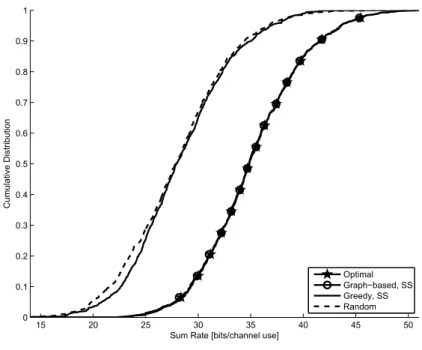
This chapter addresses distributed parameter coordination methods for wireless commu-nication systems. Two distributed algorithms for the problem of precoder selection are presented. The first and simplest method is the greedy solution in which each communication node in the network acts selfishly. The second method and the focus of this chapter is based on a message-passing algorithm, namely min-sum algorithm, in factor graphs. Three kinds of precoding code-book are considered: transmit antenna selection, fixed-beam selection, and 3GPP long-term evo-lution (LTE) precoder selection. Evaluations on the potential of such an approach in a wireless communication network are provided and its performance and convergence properties are com-pared with those of a baseline selfish/greedy approach. Simulation results are presented and discussed, which show that the graph-based technique generally obtains gain in sum rate over the greedy approach at the cost of a larger message size. For instance, the percentage gain in sum rate over the greedy is about 33% within 5 iterations in a 7-cell network considering single-layer LTE precoders. Besides, the graph-based method usually reaches the global optima in a efficient manner. Methods for improving the rate of convergence of the graph-based distributed coordination technique and reducing its associated message size are therefore important topics for wireless communication networks.
2.1 Introduction
In a cellular network, there are many occasions in which each cell needs to set a parame-ter value, such as reference signal, transmit power, beam direction, or scheduled user. This must be done in such a way that the setting in a given cell is preferably compatible with the ones of its neighboring cells in order to achieve a certain notion of optimality, such as maximizing the average system or user throughput, for the entire network [1, 2]. The choice made by one cell on a local parameter often affects the interference level experienced by its immediate neigh-bors and hence their respective choices made on their local parameters, which in turn would influence the choices made by their neighbors’ neighbors. The simplest example is perhaps the classical frequency reuse problem [3] where the frequency band in which each cell transmits or receives is preferably different from those of its immediate neighboring cells to avoid mutual interference [4].
future cellular networks, there is also an increased interest in methods of performing the coordi-nation of parameters among neighboring cells in an autonomous and distributed fashion without a central controller, as any unplanned addition (or removal) of base-stations can substantially alter the system topology and thus the preferred settings.
A distributed approach which has been extensively used in wireless communications is related to game-theoretical models [5, 6]. Since the nature of wireless communication systems is, in general, based on the optimization of conflicting cost functions, in terms of resources usage and performance achievement, a decision-making process/tool is a natural choice. Further, the cooperative or non-cooperative aspects of the elements of the system can be taken into account in order to iteratively find a proper solution. Such a proper solution, although may not be optimal, is the best solution for the overall system and a different point into the system leads the individuals to have a worst performance, in terms of the assumed metric, which is the basis of the Nash equilibrium point [7].
The number of problems which have benefited from the usage of game theory-based methods in the context of wireless systems and networks is large and extensive. Frequency reuse optimization, multiple-input-multiple-output (MIMO) precoder design, antenna selection, among others have been heavily studied in the existing literature [5, 6, 8–11]. However, on prac-tical setups, the latency of finding the Nash equilibrium point may be prohibitive and lead to a sub-optimal solution or even to a non-convergent point which is not suitable. Also, it is not always ensured that the game theory solution is a Nash equilibrium point [6]. These important issues motivate the usage of different, potentially more complex solutions in terms of signaling, distributed approaches in order to be more adequate to real scenarios.
Factor graph and the associated sum-product algorithm have been widely used in prob-abilistic modeling of the relationship among inter-dependent (random) variables or parame-ters. There are numerous successful applications [12] including, most notably, various fast-converging algorithms for decoding low-density parity check (LDPC) codes and turbo codes, generalized Kalman filtering, fast Fourier transform (FFT), etc.
One classic example motivated the most: the prisoner’s dilemma [13]. In a few words, the two prisoners find an equilibrium point if both greedily betray. However, this is not a good solution because they can individually decrease their sentences if both of them stay silent, which is the best solution and it is reached only if there is a sort of communication or centralization. In this context, the graph-based approach reaches the optimal solution by applying the message-passing algorithm.
transmit beamforming problem in a multi-cell MIMO system considering a one-dimensional cel-lular model. Moreover, in [16, 17] some message-passing algorithms (including the sum-product algorithm) are deployed to coordinate parameters of downlink beamforming in a distributed manner in a multi-cell single-input-single-output (SISO) system.
In this chapter, we focus on a method founded on factor graphs for the application of precoder selection, i.e. transmit antenna selection [18] and beam selection (including LTE precoders), in a distributed manner. Based on factor graphs, a variant of the sum-product al-gorithm [12], namely the min-sum alal-gorithm [19], can then be applied in order for all nodes, through iterative message passing with their respective neighbor nodes, to decide upon the best set of local parameters that can collectively maximize a global performance metric across the network. The algorithm allows each communication node to be indecisive of its own decision un-til sufficient information about how its decision would affect the overall network performance is accumulated. The performance of such a graph-based method along with other distributed meth-ods, e.g. game-theoretic approach [11], for coordination of discrete parameters in a wireless communication network are evaluated.
The rest of the chapter is organized as follows: Section 2.2 introduces the problem of coordinating parameters in communication networks; Section 2.3 presents the application of precoder selection as an example of parameter coordination; Section 2.4 addresses two different distributed solutions for the precoder selection problem; Section 2.5 shows several numerical results for different simulation setups regarding the precoder selection problem; and finally we conclude the chapter in Section 2.6.
2.2 Discrete Parameter Coordination Problem
Consider a communication network withN communication nodes. A communication
node described here may represent any communication device in general in a wireless com-munication network, for instance, a base-station (BS), an access node, or a UE in a cellular communication system. Let pi, fori= 1,2, . . . , N, denote a discrete parameter (or a vector of
two or more discrete parameters) of theith communication node, whose value is drawn from a
finite setPi of|Pi|possible parameter values for that node, where|Pi|denotes the cardinality
ofPi, and let
p≡[p1 p2 · · · pN
]T
be a vector collecting all the parameters in the network, where
pi ∈ Pi, i= 1,2, . . . , N.
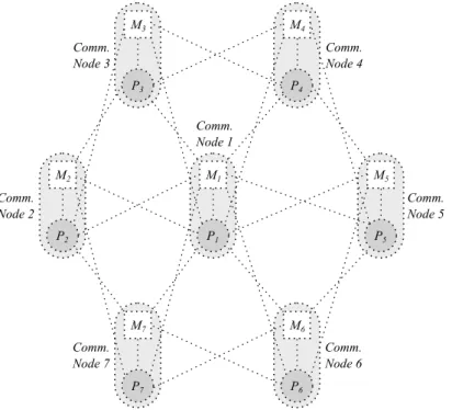
Figure 2.1 shows a hexagon layout with N = 7 communication nodes spread over hexagonal
Figure 2.1 – A general network example with a seven-cell hexagon layout. Each cell has a com-munication node which shares the set of resources available in the network.
Comm. Node 2
Comm. Node 3
Comm. Node 7
Comm. Node 5 Comm.
Node 1
Comm. Node 4
Comm. Node 6
Source: Created by the author.
to select precoding matrices [11, 20] to maximize the network throughput, and an index to a frequency band in a frequency reuse planning to minimize the number of collisions in frequency bands, just to name a few.
Each nodeiis associated with a listNiof proper neighboring nodes (i.e. excluding node
i) whose choices of parameter values can affect the local performance of nodei. For convenience,
also let
Ai ≡ Ni∪ {i}
denote the “inclusive” neighbor list or just the neighbor list of nodei. LetpAidenote the vector of those parameters of nodes inAi, with its ordering of parameters determined by the sorted indices
inAi. Associated with each nodeiis a performance metric or cost, denoted byMi(pAi), which is a function of those parameters in the neighbor listAiof nodei. Each nodeiis assumed to be
capable of communicating with all nodes inAi. The list of neighbors may simply be determined
by some metric based on the distances1among communication nodes, or, as in 4G/LTE systems,
directly accessible in a fully connected network by an X2 interface. For instance, node ican
consider its neighbors those which are distant no more than the intercell distance. Considering this distance-based metric, Table 1 shows the list of neighbors of each node iaccording to the
network in Figure 2.1.
Our goal is for each nodeito find, in a distributed fashion, its own optimal parameterp∗i,
which is the corresponding component of the optimal global parameter vectorp∗that minimizes
Table 1 – List of neighboring communication nodes of network example in Figure 2.1.
Item Neighbors list “Inclusive” neighbors list
Comm. Node 1 N1 ={2,3,4,5,6,7} A1 ={1,2,3,4,5,6,7}
Comm. Node 2 N2 ={1,3,7} A2 ={1,2,3,7}
Comm. Node 3 N3 ={1,2,4} A3 ={1,2,3,4}
Comm. Node 4 N4 ={1,3,5} A4 ={1,3,4,5}
Comm. Node 5 N5 ={1,4,6} A5 ={1,4,5,6}
Comm. Node 6 N6 ={1,5,7} A6 ={1,5,6,7}
Comm. Node 7 N7 ={1,2,6} A7 ={1,2,6,7}
the total (global) performance metric given by
M(p)≡ N
∑
i=1
Mi(pAi). (2.1)
The problem of coordinating parameters can be solved adopting basically two types of solutions: a) centralized approach, which yields the optimal global parameter vector; and b) distributed approaches, which on one hand often provide sub-optimal solutions through greedy techniques such as non-cooperative games, but on the other hand can provide near-optimal so-lutions by using a factor graph.
2.2.1 Optimal Solution: Centralized Exhaustive Search
Conceptually, the simplest approach to the discrete optimization problem described above is to solve it jointly at a central location by direct computing
pC ≡
pC,1 pC,2
· · · pC,N
≡arg min
p
N
∑
i=1
Mi(pAi), (2.2)
which is an optimal solution to the problem by definition. A major issue of this approach is its high computational complexity for large network size N, as the computational complexity
to exhaustively search the optimal solution grows exponentially as the number of communica-tion nodes increases, along with the inherent high signaling load (backhaul traffic) between the communication nodes and a central processing unit.
The computational complexity of this solution is indeed very high. The minimum (or maximum) value of a cost (utility) function is usually found enumerating all the combinations of the discrete parameters. The total number of combinations of parameterscis given by
c= N
∏
i=1
|Pi|.
For instance, if the network hasN = 61nodes and|Pi| = 3fori = 1,2, . . . , N, a number of
Figure 2.2 – An example of frequency reuse planning in a seven-cell hexagon layout. The pa-rameter vectorp = [1 3 2 3 2 3 2]T is one of the optimal solutions of the problem,
where Pi = {1,2,3}fori = 1,2, . . . ,7. That is, no collision is observed among
communication nodes.
Comm. Node 2
p2= 3
Comm. Node 1
p1= 1
Comm. Node 5
p5= 2 Comm.
Node 4
p4= 3 Comm.
Node 3
p3= 2
Comm. Node 7
p7= 2
Comm. Node 6
p6= 3
Source: Created by the author.
prohibitive. Alternatively, the exhaustive search technique may be replaced with the standard alternating-coordinate optimization technique, also known as coordinate descent, for dense net-works [21]. Such an approach starts with an arbitrary choice ofpand iteratively optimizes each element (or a particular set of elements) ofpone at a time while holding others fixed. Its conver-gence to the globally optimum result can be guaranteed under some conditions, e.g. if the cost function is somehow convexified.
2.2.2 Example Application: Frequency Reuse Planning Problem
Each parameterpimay represent an index to a frequency band out of a setPiof all
possi-ble frequency bands. The goal here is to use a distributed algorithm to solve the frequency reuse planning problem by minimizing the total number of “collisions” in terms of using the same fre-quency band in adjacent cells or BSs. Figure 2.2 shows an example of such an application where a possible optimal solution (no collision) is reached. For clarity, each one the three frequency bands correspond to a different cell color (white, light gray and dark gray) in Figure 2.2. In this case, the local performance metric may be chosen as
Mi(pAi) =
∑
j∈Ni
δ(pi, pj), (2.3)
where
δ(pi, pj) =
Specifically, there are N = 7 nodes and the parameter set of node i is Pi = {1,2,3} for
i= 1,2, . . . ,7. The solution reached is the vectorp= [1 3 2 3 2 3 2]T which causes no collision
among neighboring nodes. In other words, taking into account the neighbors list in Table 1, the solution reached leads every local performance metricMiin (2.3) to equal zero because each pair
of adjacent nodes uses different frequency bands. Consequently, the global performance metric defined in (2.1) also equals zero, which is the optimal solution for the underlying problem.
It is worth mentioning that other choices of local performance metrics are possible, which may affect the performance (e.g. faster convergence) of the algorithm in hand. One could count all “collisions” between neighboring communication nodes within the neighborhood de-fined byAi. Yet another similar metric could lead the second-tier neighbors to select the same
frequency band. However, this approach is beyond the scope of this work.
Next, the application which is the focus of this chapter, is presented along with its asso-ciated parameters and performance metric.
2.3 Precoder Selection Problem
In this section the parameter coordination problem is discussed, i.e. precoder selection, modeled by (2.1) in the context of wireless communications. Each parameterpi may represent
a PMI for BSiin the downlink (or UEiin the uplink) in a cellular network, indicating which
precoder from a predetermined set Pi of precoders or beamforming weights that BS (or UE)i
should use at a certain radio resource block to transmit signals. In practical systems, different UEs may be scheduled, and thus different precoders may be used at different radio resource blocks. In this case, the coordination of precoders may be performed independently for each individual radio resource block under some constraints.
Consider a multi-cell MIMO system in the downlink in which each BS hasNtavailable
transmit antennas and each UE has Nrreceive antennas, and there is a single UE per cell. The
BSi transmits precoded and spatially multiplexed vectorxi to its associated UEi. The vector
xiis defined as
xi =
√
1
Ns
W(pi)si,
whereNsis the number of data streams,siis theNs×1spatially multiplexed (SM) symbol vector,
andW(pi)∈ Wis theNt×Nsprecoding matrix specified by the parameterpi. Examples of set W can be a LTE precoding codebook, a fixed beamforming weights codebook, and a transmit
antenna selection (TAS) codebook. In general,W is the set of all precoding matrices available
for every communication node in the network. In order to index the elements ofW, assume an
index setI, which is equivalent toPi, defined as
Pi ≡ I ,
{
1,2, . . . ,
(
Nt
Ns
)}
for all the communication nodes. Then, a bijective function
f: Pi ↔ W (2.5)
maps the elements ofPi onto the elements ofW properly.
This work focuses on three particular examples of precoding matrix W for spatially multiplexed transmission: a) TAS precoder, b) discrete Fourier transform (DFT)-matrix-based precoder, and c) LTE precoder.
a) Transmit Antenna Selection: Let each element ofWbe anNt×Nssubmatrix of an identity
matrixINt. That is, the unique non-null entry of each column of this submatrix selects a
transmit antenna. For example, forNt= 3andNs= 2,
W = 1 0 0 1 0 0 , 1 0 0 0 0 1 , 0 0 1 0 0 1 , (2.6)
where each matrix inWis a particularWindexed bypi ∈ Pi, according to (2.4) and (2.5).
In other words, each matrixW selects two antennas out of three, where the first matrix selects antennas 1 and 2, the second matrix selects the antennas 1 and 3, and finally the last matrix selects the antennas 2 and 3.
b) Fixed-Beam Selection: Let each element ofW be anNt×Ns submatrix of theNt×Nt
DFT matrixFdefined as being
F= √1
Nt
1 1 1 · · · 1
1 w w2 · · · w(Nt−1)
1 w2 w4 · · · w2(Nt−1)
... ... ... ... ...
1 w(Nt−1) w2(Nt−1) · · · w(Nt−1)(Nt−1)
,
where w = e−2Ntπj, e is the basis of the natural logarithm and j is the imaginary unit. Basically, each matrixW changes the relative phase and direction of the vectorsto be transmitted. For instance, forNt= 3andNs = 2,
W = √1 3 1 1
1 e−2πj3 1 e−4πj3
, 1 1
1 e−4πj3 1 e−8πj3
, 1 1
e−2πj3 e−4πj3
e−4πj3 e− 8πj 3 , (2.7)
where each matrix inW, similar to the TAS case, is a particularWindexed bypi ∈ Pi,
c) LTE Precoder Selection: Let each element ofWbe anNt×Nsbe a precoding matrixW
in a matrix codebook, namely LTE precoding codebook [22], defined as a set of complex weighting matrices for combining theNsdata streams before transmission. As an example,
whenNt= 2andNs= 1, the LTE codebook is
W = 1 1 , 1 −1 , 1 j , 1 −j
, (2.8)
where each matrix inW is a particularWi indexed by pi ∈ Pi, according to (2.4) and
(2.5) as in the previous examples.
For any kind of codebook described above, the sampled incoming signal vector at the receiveriis given as being
yi =√giiHiixi+
∑
j∈Ni
√g
jiHjixj+vi, (2.9)
where Hji denotes the MIMO channel response from BSj to the UE served by BS i in the
downlink, quasi-static over a data block, andvi is a zero-mean circularly symmetric complex
Gaussian (ZMCSCG) noise vector. The constantgji is a gain that corresponds to the path loss
of each signal, here modeled in a simplified way as being
gji =
(
1
dji
)α
, (2.10)
where the constantαrefers to the path loss exponent anddjiis the distance between the
trans-mitterj and the receiveri, for each random drop of UEs in the cell grid considering fixed BSs’
positioning. The second term on the right-hand side refers to the interference caused by the neigh-boring communication nodes. For each transmitter, the average transmitted power is constant and given by
E{∥xi∥2
}
= 1
Ns
tr(WWH)=PT, (2.11)
wherePT is the transmit power in units of energy per signaling period. Also, the symbols are
assumed to be uncorrelated and have unit power, which means thatE{sisHi
}
=INs.
In both cases, the local performance metricMi(pAi)may represent the negative of the rate [8, 23] of the cell corresponding to BSimeasured by
Mi(pAi) =−log det
(
I+|gii|Ri−1HiiW(pi)W(pi)HHHii
)
, (2.12)
whereRi, defined herein as
Ri ,Rvi+
∑
j∈Ni
|gji|HjiW(pj)W(pj)HHHji, (2.13)
performance metric is simply the system capacity in the network. Hence, one may intuitively think of employing a distributed algorithm for the BS to negotiate their choices of downlink precoding matrices with their respective neighbors so that the system capacity in the network is maximized. Such approaches shall be discussed in the upcoming sections.
2.3.1 Channel Modeling: Measurements and Setup
To obtain more realistic results, each MIMO channel response was drawn from a data set Dof measured channel matrices acquired by Ericsson Research during measurement
cam-paigns made in Kista neighborhood in Stockholm, Sweden. The measurement camcam-paigns were performed using a single BS placed on the roof of a building and a UE mounted inside a van at a convenient driving speed (see more details in [24, 25]). A total of 324,000 samples of channel matrices measured along a particular route2of Kista compounds the setD. For the sake of
remov-ing any “original” large-scale fadremov-ing effect, each entry of the channel matrices was previously transformed into a zero-mean and unity-variance variable, such that
[Hji]k,l = [Dji]k,l−µD
σD
, Dji ∈ D, k= 1. . . Nr, l = 1. . . Nt, (2.14)
whereDji, randomly picked up from setD, is associated with receiverj and transmitteri,µD
andσ2
D are the mean and the variance of the entries of the matrices inD, respectively, andHji
is the transformed MIMO channel matrix also associated with receiverj and transmitteri. The
indiceskandlindex the element(k, l)of both matricesDjiandHji. Then, the path loss modeled
by the parametersgjiis in turn inserted into the matrixHjiaccording to (2.9). For convenience,
the log-normal shadowing has not been modeled in this formulation. It is worth noting that each element ofD is randomly chosen only once so that each pair of receiver and transmitter has a
different channel matrix.
To illustrate the spatial characteristics of such a channel model, consider a MIMO setup such that each transmitter has Nt = 3 antennas and each receiver hasNr = 2 antennas. The
resulting channel matrices are characterized by the presence of a number of eigenmodes less than 2. Such a feature is observed in the estimated power coupling matrix Ω[26] of resulting
MIMO channel matrices, graphically presented in Figure 2.3.
The matrixΩshows the spatial arrangement of scattering objects between the
transmit-ter and the receiver, where its columns refer to the transmit eigenmodes and the rows the receive eigenmodes. In this example, only the transmit eigenmode 1 couples to the receive eigenmodes, which is suitable for beamforming. This matrix generally characterizes the entire data setDin
the sense that all the pairs of receiver and transmitter observe spatially-correlated channels. The motivation to use such a channel model is to provide a suitable scenario for the beam selec-tion technique, which usually benefits from the characteristics of spatially-correlated channel matrices.
Figure 2.3 – Estimated power coupling matrixΩof 2x3 MIMO channel matrices. Only the Tx.
eigenmode 1 couples to the Rx. eigenmodes.
1
2
3 1
2 0 0.5 1 1.5 2 2.5 3 3.5
Tx. eigenmode Rx. eigenmode
Source: Created by the author.
Next, methods to solve the aforementioned problem in a distributed manner are shown and discussed.
2.4 Distributed Solutions to Parameter Coordination
In this section two distributed methods to the problem of parameter coordination in com-munication networks are discussed. The first one is the greedy solution, which often has a sub-optimal performance through selfish/greedy techniques such as non-cooperative games. The second method is a method based on message pass in factor graphs presented as a near-optimal solution.
2.4.1 The Greedy Method
The greedy method can solve the optimization problem described in Section 2.2 by al-lowing each communication node to selfishly set its own parameter. Then, each node optimizes its own local performance based on the most recent choices made and given by its neighbors. In this approach, the complexity of each node grows only linearly with the cardinality of the set of parametersPi since only the parameters of the node itself are considered in the local
optimiza-tion at the node. More precisely, in this approach, the local parameterpiat each communication
node is iteratively chosen as
p(S,in+1) ≡arg min pi
Mi(pAi)
pNi=p
(n)
S,Ni
(2.15)
wherenis the iteration index,p(S,in+1) denotes the choice ofpimade at iterationn+ 1using this
inNiat thenth iteration. In turn, the parameterp( n)
S,i at each node is exchanged to its neighboring
nodes so that every node obtains its parameter vectorp(S,Nn)ito compute its next parameterp(S,in+1).
Considering some simplifications, the LTE solution for precoder selection described in [20] can be seen as a single iteration of the greedy solution, particularly the first iteration. That is, such a solution is the first best response reaction in (2.15), which may be formulated as
pL,i ≡arg min pi
Mi(pAi)
pNi=p(1)S,N
i
(2.16)
wherepL,i denotes the choice ofpi using the LTE precoding solution andp(1)S,Ni corresponds to the vector of those parameter choices made by nodes inNi atn = 1in the greedy approach.
From a game-theoretic perspective, the greedy method may be seen as a non-cooperative game in which the players, i.e. the rational decision makers, are the communication nodes. Re-garding the other game components, theset of actionsmay be the setPi and theobjective func-tionmay be the local performance metricMi(pAi), both associated with (player) nodei. Con-cisely, this kind of equilibrium is established if each player has chosen an action and no one can benefit by changing its action unilaterally while the others keep theirs unmodified [13]. It is considered a predicted outcome of the game in the sense that if that outcome is reached, then no player has an incentive to deviate from it. Therefore, an action tuple{p⋆
S,i,p⋆S,Ni
}
for nodei
is a Nash equilibrium (NE) if
Mi
(
p⋆ S,i,p
⋆ S,Ni
)
≥Mi
(
pS,i,p⋆S,Ni
)
, ∀pS,i∈ Pi, i= 1,2, . . . , N. (2.17)
The superscript⋆denotes that the underlying parameter leads to a NE. The inequality above is
a convenient form for representing a NE. Throughout this chapter, the greedy method is treated as a non-cooperative game and a pure-strategy NE is defined as the game solution.
With respect to the precoder selection problem described in Section 2.3, an equilibrium point (i.e. a NE), means that each transmitter will transmit with the precoding matrix according to the game result. But a particular NE action tuple does not say anything about how this equi-librium point is reached or about uniqueness. Actually, the receivers have limited information and therefore they can not predict an equilibrium. Thus, some ”learning” algorithm must be con-cerned in order to dynamically reach an equilibrium. The process of reaching an equilibrium point is an important issue and it is usually described by a distributed algorithm. Guerreiro et al. in [11] present a distributed algorithm, namely Game-theoRetic Antenna Subset Selection (GRASS), that provides a simple (but sub-optimal) solution to the precoder selection problem (using the TAS codebook) by formulating it as a game. Such an algorithm is briefly described in the following.
2.4.1.1 GRASS Algorithm
Table 2 – Summary of the GRASS algorithm.
Steps Description
Step 0: For all communication nodes, estimateHiiand set iteration index
n = 0.
Step 1: At each communication nodei, obtain covariance matrixRi.
Step 2: At each communication nodei, compute the parameter
p(S,in+1) ≡arg min pi
Mi(pAi)
pNi=p
(n)
S,Ni
by finding the argument that minimizes the local performance met-ricMibased on the current matrixRi.
Step 3: Increment iteration indexnand go back to Step 1 unless a NE or
certain stopping criterion is satisfied.
Step 4: At each communication nodei, send the PMI associated with the
parameterp(S,in+1)back to the transmitter.
one may think of it as a particular case of the greedy method that considers the TAS codebook. The algorithm is performed at each receiver in a simultaneous manner with no coordination among the transmitters. It may be summarized (Table 2) as: (1) performing an initial step of channel estimation at the receivers in step 0; and, (2) in each of a bounded number of iterations, the nodes exchange information about the parameter selection (i.e. PMI) made for their respec-tive transmitters, with each receiver trying to reach the NE point, and with game play continuing until all nodes converge (or until a limited number of iterations is reached) in step 1 until 3. The finalized precoding matrix selection done by each receiver is sent to the transmitter associated with that receiver in step 4.