Artistic rendering of the visual cortex
Roberto Lam(1), João Rodrigues(1), and J.M.Hans du Buf(2)
(1) University of Algarve – Escola Superior de Tecnologia, 8005-139 Faro, Portugal.
(2) University of Algarve – Vision Laboratory – FCT, 8005-139 Faro, Portugal.
Abstract — In this paper we explain the processing in thefirst layers of the visual cortex by simple, complex and end-stopped cells, plus grouping cells for line, edge, keypoint and saliency detection. Three visualisations are presented: (a) an integrated scheme that shows activities of simple, complex and end-stopped cells, (b) artistic combinations of selected activity maps that give an impression of global image structure and/or local detail, and (c) NPR on the basis of a 2D brightness model. The cortical image representations offer many possibilities for non-photorealistic rendering.
Index Terms — Non-photorealistic, rendering, cortex, multi-scale.
I. INTRODUCTION
Visual perception is a very complicated process. The image that we see is a virtual representation of our environment. We can construct a global impression or gist of what is where, and we can concentrate on detail when analysing the texture of our skirt or trousers. Important objects like faces immediately pop out, which points at parallel processing, whereas serial processing is necessary when comparing minute differences of two textures.
Apart from image processing and computer graphics, i.e. surface and volume rendering, an important research topic of our Vision Laboratory concerns the development of models of the visual system for the prediction of detection and brightness data as measured by psychophysical experiments [1], [4], [5]. Such models are based on cortical simple and complex cells (anisotropic filters), for which Gabor wavelet kernels are employed. Recently, models of other cortical cells have been developed, for example bar and grating cells [14], [20] and end-stopped cells [7], [16], the first detecting isolated bars or periodic structures, the latter junctions and points of high curvature (keypoints).
Apparently, the retinotopic projections in the hypercolumns of cortical area V1 can be as a huge data explosion: simple and complex cells are tuned to different frequencies (scales, Level-of-Detail) and orientations, and these are used for the coding of lines and edges. End-stopped cells group outputs of complex cells for coding keypoints, including junction type (L, T, +, etc.). In turn, outputs of end-stopped cells can be grouped over scales in order to create saliency maps for Focus-of-Attention (FoA) [8], [12], [17], a process that the visual system uses
in the selecting the most important (or complex) spots for focusing the eyes.
In view of the huge amount of data, the development of optimised detectors (lines, edges, keypoints, even motion and disparity) is difficult because the multi-scale representations cannot be visualised efficiently for analysing what happens in the case of real images. This requires new multi-dimensional visualisation techniques. In addition, instead of only displaying cortical image representations, new non-photorealistic rendering (NPR) methods can be developed. For an indexed NPR taxonomy see [21]. The ultimate goal may be to develop more intelligent filters for GNU’s GIMP and Jasc Software’s Paint Shop Pro, for example a “van Gogh filter” which can simulate his typical impressionist style.
Trying to understand painters, their techniques, and visual aesthetics in general, is a challenge, especially when referring to physical processes in the eyes and brain [11], [24]. An even bigger challenge is to exploit these physical processes in trying to simulate techniques of certain painters. This requires state-of-the-art models of visual representations in the visual cortex together with insight in high-level cognitive processes.
In this paper we show one visualisation approach, in the line of Kruger’s symbolic pointillism [9]. We also show that the many different image representations and feature maps in the cortex can be artistically combined for non-photorealistic rendering purposes. This includes the use of an actual brightness perception model to produce an impressionist oil painting. In Section 2 we present the models of simple, complex and end-stopped cells. Section 3 deals with the visualisation of cortical maps, and Section 4 with non-photorealistic rendering. We conclude with a small Discussion (Section 5). Note: readers not familiar with mathematics can jump to the second-last paragraph of Section 2.
II. CELL MODELS AND NCRFINHIBITION
Gabor quadrature filters provide a model of cortical simple cells [10]. In the spatial domain (x, y) they consist of a real cosine and an imaginary sine, both with a Gaussian envelope. A receptive field (RF) is denoted by (see e.g. [6]):
, ~ 2 cos 2 ~ ~ exp ) , ( 2 2 2 , , , ⎟ ⎠ ⎞ ⎜ ⎝ ⎛ + ⎟ ⎟ ⎠ ⎞ ⎜ ⎜ ⎝ ⎛ + − = ϕ λ π σ γ ϕ θ σ λ x y x y x g (1) , sin cos ~ ; sin cos
~x=x θ+y θ y=y θ−x θ where the aspect ratio γ = 0.5 and σ determines the size of the RF. The spatial frequency is 1/λ, λ being the wavelength. For the bandwidth σ/λ we use 0.56, which yields a half-response width of one octave. The angle θ determines the orientation (we use 8 orientations), and φ the symmetry (0 or π/2). We apply a linear scaling between fminand
max
f with a few discrete scales, or hundreds of contiguous scales.
The responses of even (Fig. 1(A)) and odd (Fig. 1(B)) simple cells, which correspond to the real and imaginary parts of a Gabor filter, are obtained by convolving the input image with the RF, and are denoted by RsE,i(x,y) and RO, (x,y)
i
s , s being the scale and i the orientation
(
θi =iπ (Nθ−1))
and N the number of orientations. In θorder to simplify the notation, and because the same processing is done at all scales, we drop the subscript s. The responses of complex cells (Fig. 1(C)) are modelled by the modulus
( )
,{
( )
,}
{
( )
,}
2. 1 2 2 ⎥⎦ ⎤ ⎢⎣ ⎡ + = R x y R x y y x C O i E i i (2)There are two types of end-stopped cells [7], [23], i.e. single (S) and double (D), see Fig. 1(D) and (E), respectively. If
[]
. denotes the suppression of negative + values, and Cˆ =i cosθi and Sˆ =i sinθi, then(
)
[
(
ˆ , ˆ)
]
; ˆ , ˆ ) , ( + + − − − + = i i i i i i i C d y S d x C C d y S d x C y x S (3)( )
(
)
[
− + − − = i i i i i x y C x y C x dS y dC D ( , ) , 12 2 ˆ , 2 ˆ]
. ) ˆ 2 , ˆ 2 ( 12 − + + i i i x dS y dC C (4)The distance d is scaled linearly with the filter scale s, i.e. d=0.6s. All end-stopped responses along strait lines and edges need to be suppressed, for which we use tangential (T) and radial (R) inhibition (Fig. 1(F) and (G)):
( )
[
( )
(
ˆ , ˆ)
]
; , , mod 1 2 0 mod + − = + + + − =∑
i i N i N i i N T S d y C d x C y x C y x I θ θ θ (5)( )
[
( )
, ˆ 2 , ˆ 2 . 4 , , mod ) 2 ( 1 2 0 mod + + − = ⎥ ⎦ ⎤ ⎟ ⎠ ⎞ ⎜ ⎝ ⎛ + + − =∑
i i N N i N i i N R S d y C d x C y x C y x I θ θ θ θ (6)where
(
i+Nθ 2)
modNθ ⊥imodNθ.The model of non-classical receptive field (NCRF) inhibition is explained in more detail in [6]. We will use two types: (a) anisotropic, in which only responses obtained for the same preferred RF orientation contribute to the suppression, and (b) isotropic, in which all responses over all orientations equally contribute to the suppression.
The anisotropic NCRF (A-NCRF) model is computed by an inhibition term A
i s
t ,σ, for each orientation i, as a convolution of the complex cell response Ci with the
weighting function wσ, with
( )
[
]
[
( )
]
1 , , ) , (x y = DoG x y + DoG x y + wσ σ σ , (7) 1 .being the L1 norm, and
( )
( )
( )
. 2 exp 2 1 4 2 exp 4 2 1 , 2 2 2 2 2 2 2 2 ⎟ ⎟ ⎠ ⎞ ⎜ ⎜ ⎝ ⎛ + − − ⎟ ⎟ ⎠ ⎞ ⎜ ⎜ ⎝ ⎛ + − = σ πσ σ σ π σ y x y x y x DoG (8) The operator A i sb ,σ, corresponds to the inhibition of Cs,i,
i.e. , , =
[
, − A, ,]
+, i s i s A i s C tb σ α σ with α controlling the
strength of the inhibition.
The isotropic NCRF (I-NCRF) model is obtained by computing the inhibition term tsI,σwhich does not
dependent on orientation i. For this we construct the maximum response map of the complex cells
{ }
sis C
C~ =max , with i=0,...Nθ−1. The isotropic inhibition
term tsI,σis computed as a convolution of the maximum
response map Cs
~
with the weighting function wσ, and the
isotropic operator is , =
[
~ − I,]
+. s s I s C t b σ α σWe use NCRF inhibition to suppress keypoints which are due to texture, i.e. textured parts of an object surface. We experimented with the two types of NCRF inhibition introduced above, but here we only use the best results which were obtained by I-NCRF at the finest scale.
All responses of the end-stopped cells
( )
∑
−( )
= = 1 0 , , Nθ i Si x y y x S and( )
∑
−( )
= = 1 0 , , Nθ i Di x y y x D areinhibited in relation to the complex cells (by bsI,σ), i.e. we
that are above small threshold of bsI,σ. Then we apply
R T I
I
I= + for obtaining the keypoint maps
( )
x y S( )
x y I( )
x yKS , = ~ , −g , and KD
( )
x,y =D~( )
x,y −( )
x y I ,g , with g≈1.0, and then the final keypoint map
( )
x y{
K( )
x y K( )
x y}
K , =max S , , D , .Fig.1. 2D and 3D plots of RFs of even (A) and odd (B) simple cells, complex cells (C), and 2D plots of single (D) and double (E) end-stopped cells, plus schemes for tangential (F) and radial (G) inhibition.
In multi-scale case keypoints are detected the same way as done above, but now by using KsS
( )
x,y =( )
x y I( )
x ySs , −g s , and KsD
( )
x,y = Ds( )
x,y − gIs( )
x,y .For more details and results see [17].
An important aspect in any observation scheme is Focus-of-Attention by means of a saliency map [8], [18], i.e. the possibility to draw attention to and to inspect, serially or in parallel, the most important parts of faces [19], objects or scenes [17]. In terms of visual search, this includes overt attention and pop-out. If we assume that retinotopic projection is maintained throughout the visual cortex, the activities of all keypoint cells at the same position (x, y) can be easily summed over scale s, which leads to a very compact, single layer map. At the positions where keypoints are stable over many scales, this summation map, which could replace or contribute to a saliency map [12], will show distinct peaks at centres of objects, important sub-structures and contour landmarks. The height of the peaks can provide information about the relative importance. In addition, this summation map, with some simple processing of the projected trajectories of unstable keypoints, like a dynamic lowpass filtering related to the scale and non-maximum suppression, might solve the segmentation problem: the object centre is linked to important sub-structures, and these are linked to contour landmarks. Such a mapping or data stream is data-driven and bottom-up, and could be combined with top-down processing from inferior temporal cortex (IT) in order to actively probe the presence of certain objects in the visual field [2]. In addition, the summation map with links between the peaks might be available at higher brain areas where serial processing occurs for e.g. visual search. An important aspect of visual representation is line/edge detection and classification. Rodrigues and du Buf [15], [16] presented a scheme for line and edge detection based on the responses of simple and complex cells, i.e. simple cells serve to detect positions and event types, whereas complex cells are used to increase the confidence. A positive line is detected where RE shows a local
maximum in the filter orientation and O
R shows a zero crossing. In the case of an edge the even and odd responses must be swapped. This gives 4 possibilities for positive and negative events: local maxima/minima plus zero crossings. Since the use of Gabor modulus (complex cells) implies some loss of precision at vertices [3], increased precision is obtained by considering multiple scales. A more detailed description of line and edge detectors is beyond the scope of this paper. We refer to [22] for a discussion of complicating factors such as the size of receptive fields in the case of curved lines and edges.
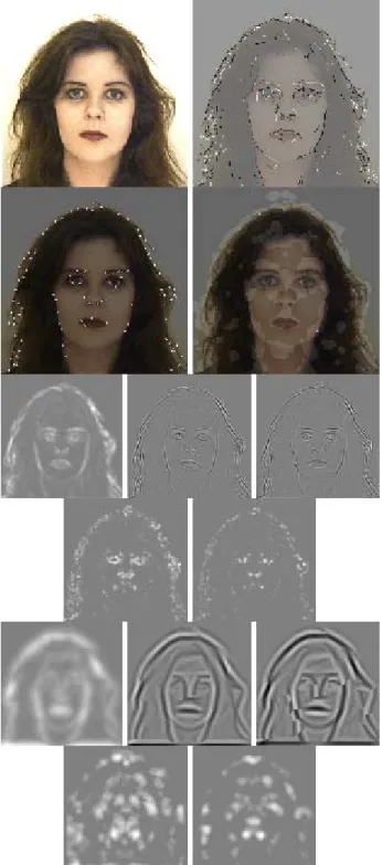
Figure 2 shows, from top to bottom, input image (Fiona), an event map that combines the positions and types (coded in gray level) of lines and edges, keypoints with I-NCRF inhibition, a saliency map, then activities of complex cells, even and odd simple cells, plus single and
double end-stopped cells. Apart from the saliency map, which combines keypoints over a big scale interval (λ = [4, 24]), the images show the information only at the finest scale (λ = 4).
Fig. 2. Fiona image with line/edge, keypoint and saliency maps, plus simple, complex and end-stopped cell responses (see text).
The bottom two rows show complex, simple and end-stopped cells at a coarser scale (λ = 16). Complex and simple cell activities are only shown for the local dominant orientation, i.e. this is a selection of all cell activities.
In summary, cortical area V1 contains a stack of scale- and/or orientation-tuned cells that provide image representation and feature maps: even and odd simple cells, complex and end-stopped cells, plus many grouping cells that detect basic features like lines and edges, bars and gratings, keypoints and saliency maps for FoA, probably also motion and disparity.
III. VISUALIZATION
In all simulations we assume that there exist simple, complex and end-stopped cells at all pixel positions. An advantage of this choice is that cell responses at different scales can be visualised using the same zoom factor. Here we present one scheme for visualising activities of even and odd simple cells, complex cells, single and double end-stopped cells, plus the saliency map, using different colours, the saturation corresponding to a cell’s amplitude. In addition, the dominant local orientation, which corresponds to the orientation of the complex cell with maximum amplitude, is coded by rotating the “colour wheels”.
Figure 3 shows the scheme in the case that the dominant local orientation is horizontal. The coloured circle is subdivided into four quadrants, and one quadrant is further divided into two octants. The red and blue quadrants show even (B) resp. odd (F) simple cells, the green (A) quadrant showing complex cells. The line (D) separating the two pinkish octants shows the dominant orientation (here horizontal). The upper and lower octant show single (C) and double (E) endstopped cells. The black dot (G) in the centre of the coloured circle shows the information in the saliency map (detected keypoints). The advantage of using colour saturation is that complex cells (green) with very low activity are displayed as white; hence, areas with no green component do not contain significant lines and edges, and therefore also no keypoints. In contrast, responses of even and odd simple cells can be positive or negative (white indicates a large
but negative amplitude). Finally, the coloured circles can be superimposed on the input image in order to see (part of) the underlying image structure.
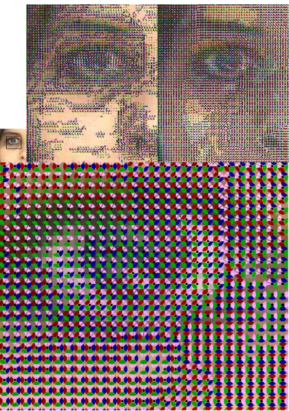
Figure 7 shows a real example, i.e. the area around one eye of Fiona, at scales λ = 4 (left) and λ = 16 (right), the atter being zoomed at the bottom, which shows only the area around the pupil. The bottom image is aesthetically appealing, we can recognise the image structure, and we can see the cell responses in order to optimise the basic line, edge and keypoint detection schemes.
IV.NON-PHOTOREALISTIC RENDERING
The many cell layers highlight different image representations: the basic activities of simple, complex and end-stopped cells, and the extracted feature maps that include lines, edges, keypoints and saliency. All is done in scale, and simple and complex cells also in multi-orientation. This host of information offers many possibilities for non-photorealistic rendering, by selecting some maps, attributing false colours, and combining them with different weight factors. It is impossible to present all possibilities, hence we simply present a few examples in Figs 8 and 9.
In all cases, non-photorealistic images were created from three different images that provide input for the RGB colour channels. To each image is attributed a weight. One additional image, the saliency map, is used to highlight the colours at salient positions where there are important keypoints.
In Fig. 8 (top row), the first image corresponds to detected lines and edges by complex cells at the finest scale (λ = 4), the second is a combination of line/edge detection and classification at two different scales (λ = 4 and λ = 16), after lowpass filtering by a Gaussian function, with an emphasis on the coarse scale. The third is a combination of even and odd simple cell responses, again at two different scales (λ = 4 and λ = 16), but this time with an emphasis on the fine scale. The four bottom images show results obtained with different weight factors and by using the three images differently in the RGB channels. Figure 9 shows more results obtained with different input images.
Instead of only using cortical feature maps, we can go one step further and exploit a model of brightness perception. To understand this, it is important to realise that our visual system does not reconstruct the visual input: there is no cell layer with a 2D brightness map, because this would require yet another “observer” in our brain. The image that we perceive is virtually constructed by a learned interpretation of cell activities in area V1 and beyond. Our model [4], which is being extended from 1D
to 2D, and which requires the feature extraction layers described in Section 2, is based on a very simple assumption: a responding “line cell” implies that, at its retinotopic position, there is a line with a certain orientation, amplitude and scale, the scale being interpreted as a Gaussian cross-profile with a size (σ) that depends on the scale of the underlying simple and complex cells. The same happens in the case of a responding “edge cell,” but with a bipolar cross-profile that can be simulated by a Gaussian-truncated error function: positive on one side and negative on the other. This symbolic interpretation model can be used to explain brightness induction effects, i.e. simultaneous contrast (Fig. 4) and assimilation (Fig. 5). Furthermore, the fact that simple and complex cells cannot distinguish between lines and ramp edges leads to a very elegant explanation of Mach bands, an effect that very few models can explain [13].
In terms of NPR, line and edge cross-profiles can be seen as brushes, the strokes being defined by the continuous positions along detected lines and edges. Brush size is defined by the scale of simple and complex cells, and amplitudes of complex cells can be used to modulate paint (hue, saturation, value). Using GNU’s GIMP, only four layers and RGB values that were picked from a colour image (Fig. 10 left), we created an impressionist rendering (Fig. 10 right) with absolutely no manual editing. The texture of the oil canvas is a standard GIMP feature. As can be seen, global structures (trees, lawn) have been preserved, but unimportant detail (exact crown of pine tree) has been changed. The reason lies in the selection of the input images used in the four layers: we selected a few representation scales, see Fig. 6. The more scales (layers) are used, the more realistic the rendering will be.
V.DISCUSSION
In this paper we presented an overview of the processing in the visual cortex. The many cell layers, activity and feature maps naturally invite for experiments with non-photorealistic rendering. We illustrated this by combining some cell activities into an integrated scheme, the “colour wheels,” and by combining a selection of entire maps. In the latter case entire maps are coded in false colour, possibly after postprocessing like lowpass filtering. In contrast to visual perception, in which all feature maps are somehow combined in order to “render” a realistic impression of our visual environment, a process which is not yet well understood, there seem to be no artistic limitations. Further progress in the development of additional cell models, for example for extracting motion
and disparity (depth by stereo), will provide even more possibilities, including 3D rendering with motion vectors on top of normal surface rendering (shading). With respect to exploiting our brightness model [4], but extended to two dimensions, there are many possibilities for NPR. We can select all or only a few scales. We can render these with symbolic line/edge profiles (Fig. 10) or with simulated, continuous brush strokes along lines and edges. In the future it will be possible to simulate discrete brush strokes by using randomly selected positions, also randomly varying positions, orientations and intensities (colours). It may be possible to exploit saliency maps and to model FoA in order to select regions or to modify rendering techniques in certain regions, for example the level of detail of faces, which can already be detected on the basis of multiscale keypoints [19].
However, instead of applying a certain effect at all image positions, like GIMP’s randomised brush strokes that can be influenced by image intensity or the canvas texture used in the tree image, more intelligent filters can be developed. For example, developing a “Seurat filter” might be relatively straightforward because of the fine brush strokes (“sampling”), but a “van Gogh filter”
requires, apart from knowledge about brushes and colours, deep insight into his cognitive perception [11], [24].
Fig. 5. Brightness induction 2: assimilation in which the background pulls brightness in the same direction. Top: Munker-White effect in which all gray bars have the same reflectance. Bottom: model prediction.
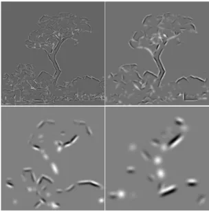
Fig. 6. The four line/edge representations of the tree image (Fig. 10 left) used to render the oil canvas (Fig. 10 right).
Fig. 4. Brightness induction 1: simultaneous contrast in which the background pushes brightness in the opposite direction. Top: all circular patches have the same reflectance. Bottom: model prediction.
AKNOWLEDGMENTS
The Fiona image is from the Psychological Image Collection (http://pics.psych.stir.ac.uk/) at Stirling University.
This investigation is partly financed by PRODEP III Medida 5, Action 5.3, and by the FCT program POSI, framework QCA III.
REFERENCES
[1] U. Bobinger and J.M.H. du Buf. In search of the holy grail: a unified spatial detection model. 25th Europ. Conf. Visual
Perception. Perception Vol. 31, Supplement, p. 137, 2002.
[2] G. Deco and E.T. Rolls. A neurodynamical cortical model of visual attention and invariant object recognition. Vision
Res., (44):621–642, 2004.
[3] J.M.H du Buf. Responses of simple cells: events, interferences, and ambiguities. Biol. Cybern., 68:321–333, 1993.
[4] J.M.H du Buf and S. Fischer. Modeling brightness perception and syntactical image coding. Optical Eng., 34(7):1900–1911, 1995.
[5] J.M.H du Buf and J. Rodrigues. Simple brightness models with lowpass and Gabor filters. 23rd Europ. Conf. Visual
Perception. Perception Vol 29, Supplement, p. 52, 2000.
[6] C. Grigorescu, N. Petkov, and M.A. Westenberg. Contour detection based on nonclassical receptive field inhibition.
IEEE Tr. IP, 12(7):729–739, 2003.
[7] F. Heitger et al. Simulation of neural contour mechanisms: from simple to end-stopped cells. Vision Res., 32(5):963– 981, 1992.
[8] L. Itti, C. Koch, and E. Niebur. A model of saliency-based visual attention for rapid scene analysis. IEEE Tr. PAMI, 20(11):1054–1259, 1998.
[9] N. Krüger and F. Wörgötter. Symbolic pointillism: Computer art motivated by human perception. Proc. Symp.
Artif. Intell. and Creativity in Arts and Science – AISB 2003, pages 36–40, 2003.
[10] T.S. Lee. Image representation using 2D Gabor wavelets.
IEEE Tr.PAMI, 18(10):pp. 13, 1996.
[11] M. Livingstone. Vision and art: the biology of seeing.
Abrams, New York (NY), 2000.
[12] D. Parkhurst, K. Law, and E. Niebur. Modelling the role of salience in the allocation of overt visual attention. Vision
Res., 2(1):107–123, 2002.
[13] L. Pessoa. Mach bands: how many models are possible? Recent experimental findings and modeling attemps. Vision
Res., 36:3205–3227, 1996.
[14] N. Petkov and P. Kruizinga. Computational models of visual neurons specialised in detection of periodic and aperiodic visual stimuli. Biol.Cybern., 76:83–96, 1997. [15] J. Rodrigues and J.M.H. du Buf. Vision frontend with a new
disparity model. Early Cognitive Vision Workshop, Isle of
Skye, Scotland, 28 May - 1 June 2004.
[16] J. Rodrigues and J.M.H. du Buf. Visual cortex frontend: integrating lines, edges, keypoints and disparity. Proc. Int.
Conf. Image Anal. Recogn., Springer LNCS 3211(1):664–
671, 2004.
[17] J. Rodrigues and J.M.H. du Buf. Multi-scale cortical keypoint representation for attention and object detection.
2nd Iberian Conf. on Patt. Recogn. and Image Anal., Estoril, Portugal (accepted), 7-9 June 2005.
[18] J. Rodrigues and J.M.H. du Buf. Multi-scale keypoint hierarchy for focus-of-attention and object detection.
Submitted to: 26th Europ. Conf. Visual Perception, A Coruña (Spain), 22-26 August 2005.
[19] J. Rodrigues and J.M.H. du Buf. Multi-scale keypoints in V1 and face detection. Accepted for: 1st Int. Symp. Brain,
Vision and Artif. Intell.,Naples (Italy), 19-21 October 2005.
[20] L.M. Santos and J.M.H. du Buf. Identification by Gabor features. Chapter 10 in: Automatic diatom identification, du Buf, H. and Bayer, M.M. (eds), World Scientific. pages 187–220, 2002.
[21] M. Sousa. Theory and practice of non-photorealistic graphics: Algorithms, methods, and production systems.
Course Notes for SIGGRAPH2003
http://pages.cpsc.ucalgary.ca/˜mario/.
[22] J.H. van Deemter and J.M.H. du Buf. Simultaneous detection of lines and edges using compound Gabor filters.
Int. J. Patt. Rec. Artif. Intell., 14(6):757–777, 1996.
[23] R.P. Würtz and T. Lourens. Corner detection in color images by multiscale combination of end-stopped cortical cells. Image and Vision Comp., 18(6-7):531–541, 2000. [24] S. Zeki. Inner vision: an exploration of art and the brain.
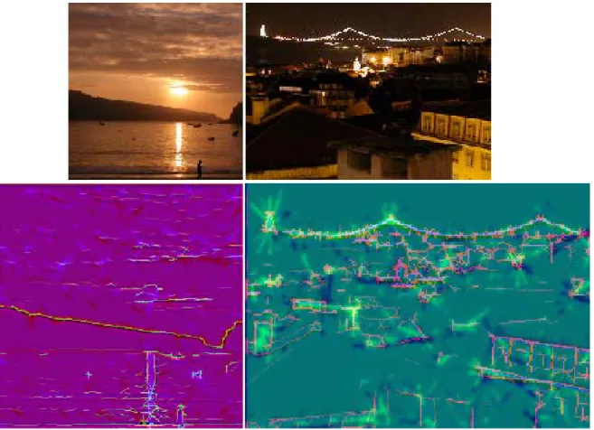
Fig. 9. Non-photorealistic rendering of sunset in São-Martinho-do-Porto and Lisbon view seen from Chapito.