http://dx.doi.org/10.1590/0103-6513.200015
1. Introduction
Biodiesel is gaining importance due to its environmental and economic benefits (Leão et al., 2011). It can replace diesel fuel without causing any harm to conventional diesel engines while reducing hazardous exhaust emissions (Van dyne et al., 1996). Zhang et al. (2003) affirmed that biodiesel is biodegradable and non-toxic and that its combustion emission profile is environmentally friendly compared to petroleum-based diesel. Van dyne et al. (1996) and Severo et al. (2015) reported the economic and environmental benefits of replacing fossil fuels with biodiesel. Biodiesel is a renewable natural resource that can help Brazilian farmers. To promote regional development, the Brazilian Biodiesel Program (BBP) was launched in 2004. This program guarantees
the purchase of a fixed amount of production from small farmers in poor communities. The ultimately goal of the program is to promote social inclusion and prosperity for these farmers by using their production in the Brazilian biodiesel supply chain (PNPB, 2013). The success of this program depends on a well-developed supply chain logistics that includes better planning and new facilities. It will also require investment in new grain crushing units, improved crop production, and a crop distribution system (Leão et al., 2011). The importance of biodiesel has also been emphasized by Carraretto et al. (2004), Demirbas & Balat (2006), Haas et al. (2006), Leduc et al. (2009) and Sotoft et al. (2010).
Received: Sept. 23, 2015; Accepted: June 16, 2016
A three-stage stochastic optimization model
for the Brazilian biodiesel supply chain
Pedro Sennaa*, Denis Pinhab, Rashpal Ahluwaliab, Julio Cesar Guimarãesc, Eliana Severoc,
Augusto Reisd
aCentro Federal de Educação Tecnológica, Nova Iguaçu, RJ, Brasil bWest Virginia University, Morgantown, Estados Unidos da América
cFaculdade Meridional, Passo Fundo, RS, Brasil
dCentro Federal de Educação Tecnológica, Rio de Janeiro, RJ, Brasil *[email protected]
Abstract
The Brazilian program for biodiesel use highlights the production of biodiesel from castor seeds. Biodiesel is a non-polluting energy source that has the potential to promote prosperity by creating jobs in poor regions of Brazil. However, the infrastructure, logistics, and proper facilities are lacking. A variety of approaches to optimizing the biodiesel supply chain have been proposed. The goal is to minimize the grain storage and transportation costs. This paper presents a comparison between a two-stage model and a multistage (three-stage) stochastic model to optimize the biodiesel supply chain. The comparison between these formulations shows that the flexibility gain provided by the multistage model results in a lower total logistic cost. The optimum for the three-stage model was 7,700,019 (BRL), compared to 8,628,002 (BRL) for the two-stage model, representing a savings of 927,983 (BRL). We highlight that this model offers a real solution for castor supply chain design (considering uncertainty) in the Brazilian semiarid region, which is a poorer region of the country, thus making cost reduction mandatory.
Keywords
Many authors have worked on developing optimization models for the biodiesel supply chain. The mathematical formulation of the problem is difficult due to uncertainties in crop production. The stochastic optimization model was first introduced by Dantzig (1955), and several other authors, including Hoffman & Schniederjans (1994), Birge & Louveaux (1997), Jayaraman (1998), Haneveld & Vlerk, (1999), Beraldi et al. (2000), Riis & Andersen (2005), Falasca
& Zobel (2011), Oliveira & Hamacher (2012) and Zhang et al. (2012), have developed optimization models that consider uncertainty. Lee (2014) and Xie et al. (2014) proposed two and multistage Mixed-Integer Linear Program (MILP) formulations to optimize the biodiesel supply chains.
This paper proposes a three-stage model to optimize the biodiesel supply chain. The objective is to minimize the costs associated with grain storage and transportation to the crushing plant. Usually, two-stage stochastic models are the most common models in the literature. Nagar & Jain (2008) affirmed that deterministic optimization models do not capture the truly dynamic behavior of most real-world applications; thus, by adding another decision stage, a model could be made more realistic. The results obtained using the three-stage model are compared with those of the two-stage model. Multistage models extend the two-stage stochastic programming models by allowing revised decisions in each time stage based on the uncertainty realized so far (Ahmed et al., 2003). For the problem shown in this paper, adding one extra decision stage allows the model to open or close facilities depending on how large the demand is. Such a flexibility gain was also highlighted by Nagar & Jain (2008), who noted that the advantage of the multistage programming approach is that we can revise parameters when more information regarding the demand scenarios becomes available. Thus, this paper yields a multistage stochastic approach applied to a castor-based biodiesel supply chain. The study helps resolve an issue that matters to Brazil as a whole, i.e., the search for cleaner fuels. In this sense, it is essential to structure the castor-based biodiesel chain because a gain in efficiency regarding the production of this fuel increases the profit margin of the chain as a whole. This paper also offers a contribution to the field of social responsibility by helping the company in question purchase the produce of small farmers, thereby reducing the logistics costs of an operation that often has little transportation scale. For this reason, the strategic positioning of facilities to help consolidate this production constitutes an important solution.
The rest of the paper is organized as follows. Section 2 provides the mathematical models, section 3 presents the problem statement, section 4 details the case study, section 5 show the main results and discussion and section 6 presents the conclusions.
2. Mathematical models
2.1. Two-stage models
The two-stage stochastic formulation can be stated as follows:
( ) ( )
{
}
M in ,
. . 0
T
x X Z x C x E Q x
S T Ax b
x
ξ ξ
∈ = +
≤ ≥
Where Q (x, ξ) is the optimum value for the second stage problem. M in . . 0 T
x Xq y
S T Wy h Tx
y ∈
≤ − ≥
x ∈ℜn is the first-stage decision variables vector.
C ∈ℜn, b ∈ℜn and A ∈ℜmx n are data associated with
the first-stage problem, y ∈ℜm is the second-stage
variable vector and ξ = (q,T,W,h) contains data for the second-stage problem, which can be random variables with known probability distributions.
Kaut & Wallace (2007) affirmed that except for very simple cases, this model cannot be solved with continuous distributions; thus, solving methods requires discrete distributions. Moreover, the cardinality of the support of the discrete distributions is limited by both the available computing power and the complexity of the decision model. Hence, in most practical applications, the distributions of the stochastic parameters must be approximated by using discrete distributions with a limited number of outcomes. The discretization is usually called a scenario tree or an event tree.
We assume, then, that each ξk,k = 1,...,ω have probabilities pk,k= 1,...,ω. So, expected value E [Q (x, ξ) can be rewriten as:
( ) ( )
1
, ,
E Q x p Qω ω x ω
ω
ξ Ω ξ
=
=
∑
Considering the discrete model, we can rewrite as follows:
( ) ( )
1
M in ,
. . 0
T
x X Z x c x p Q x
S T Ax b x
ω ω ω
Where Q (x, ξ) is the optimum value of second stage problem for each ω = 1, ..., Ω
M in
. .
0 T
x Xq y
S T W y h T x y
ω ω
ω ω ω ω
ω ∈
≤ − ≥
The first stage is responsible for “here and now” decisions based on information that we have today. These decisions correspond to the vector x. In the second stage, when ξ information is available, we make decisions regarding the values of vector y. In the first stage, we minimize the costs cTx plus
the expected value of the second-stage problem. The decisions made in the second-stage problem consist of a “course correction” in a situation in which we are able to change the decisions that are made before uncertainty is revealed. The constraints that ensure that the first-stage decisions depend only on information that is available to that point are called nonanticipativity constraints. In two-stage problems, this implies that the decision is independent of second stage realizations; thus, vector x is the same for all possible events that may occur in the second-stage problem (Birge & Louveaux, 1997).
Generally, stochastic models present a complexity that makes their resolution difficult. Ribas (2008) stated that it is common to opt for a deterministic model solution by using the average of random variables or solving a deterministic problem for each scenario. In this sense, Birge & Louveaux (1997) presented two indicators: the value of the Stochastic Solution (VSS) and Expected Value of Perfect Information (EVPI).
2.2. Multistage models
The linear multistage stochastic program is a stochastic sequential optimization where the objective function and constraints are linear (Casey & Sen, 2005). In many different ways, authors have used the multistage stochastic program approach. For example, Nagar & Jain (2008) used a scenario-based approach to address the supply chain planning problem under an uncertain environment and stated that the use of a multistage approach can generate significant savings in such problems.
For Sahinidis (2004), although significant advances have been made regarding the stochastic two-stage model solution, multistage still features a significantly considerable computational challenge compared with deterministic models; thus, a better understanding of the problem is necessary for the successful implementation of solution algorithms.
According to Casey & Sen (2005), such models are typically presented in two ways:
• MSP (Multistage Stochastic Programs)
• SDP (Stochastic Dynamic programs)
Although the SDP can often be a suitable approach for some situations, realistic applications require a much larger quantity of variables than SDP can handle efficiently. For this reason, in real-world, large-scale applications, MSP offers a more suitable modeling tool. However, MSP has computational limitations, such as the discretization of stochastic processes representing the evolution of random data (Casey
& Sen, 2005).
The multistage program with fixed recourse has the following form, as seen in Birge & Louveaux (1997):
( ) ( ) ( ) ( )
2
1 1 2 2
M in H H H
x∈X Z=c x +Eξ min c ω x+…+ω Eξ min c ω x…ω
1 1 1
. . ,
S T W x = ≤h b
( )
( )
( )( )
( )
( )
( )1 1 2 2 2 2
1 1 1
,
,
H H H H H H H
T x W x h
T x W x h
ω ω ω
ω ω ω ω
− − − + = … + = 1 0, x ≥
( )
0,t t
x ω ≥
2, ;
t= …H
Where c is a ℜn1 vector, h is a ℜm1 vector, T is a ℜm-1 vector, W is a m x n matrix and ξ = (c,h,T,W).
3. Problem statement
bases are perennial and have a greater storage capacity compared with the procurement point’s facilities. Fixed bases have higher operating costs due to their size and equipment. Moreover, fixed bases have a long-term agreement, which results in a higher rental cost. Procurement points are flexible and smaller facilities that can be moved from their current locations to a different one depending on a manager’s decisions. They have lower storage capacity and are less costly. Thus, the decisions to be made include i) where warehouses should be located, ii) which type of warehouse (fixed bases or procurement points) is more efficient in that location, and iii) what amount of castor seed must be transported from farms to warehouses and from warehouses to the plant. Furthermore, uncertain production quantities add to problem complexity; thus, using a deterministic approach provides a supply chain design only for one specific scenario. Therefore, to increase accuracy, the mathematical model should consider uncertainties, which means that a fairly good solution for some scenarios will be given instead of an optimal solution that perfectly matches one single scenario. Uncertainties are mainly due to weather conditions, such as rainfall, that impact seed production.
The proposed model to support the decision-making process is based on a three-stage stochastic MILP. The real-life biodiesel case study presented in this paper can be classified as a network location-allocation model that is represented by directed graphs. The nodes of the graph represent
i) producing cities, ii) cities that are candidates to have warehouses and iii) the city in which the plant is located. To model this problem as a multistage stochastic MILP, the proposed logistics network was created with two distinct sets of arcs: primary and secondary flow arcs. Primary flow arcs are those that connect farmers to the warehouses, and secondary flow arcs connect the warehouses to the crushing plant. This model minimizes the transportation costs, costs involved in loading and unloading trucks with castor seeds and costs associated with the installation of castor seed warehouses. The composition of these three costs form the objective function of the problem. The proposed mathematical model ultimately aims to find i) the warehouse locations and their types, ii) the quantity of castor seed flow between cities, and iii) the quantity of castor seeds flow between warehouses and crushing plants. Data used in this paper can be seen in the Appendix A.
3.1. Two-stage approach
In both two- and multistage models, we consider a horizon of three time periods, with each period corresponding to a year in which the operation of two consecutive harvests is planned. Period t = 0 represents an earlier period, where allocation decisions are made before harvesting.
Once built, these facilities will be used in the next harvest, i.e., farmers in period t will use the facilities built in t - 1.
Notations: Sets and indexes
f ∈ F Distance range
i,j,l ∈ L Cities
k ∈ K Facility type
p ∈ P Product
t ∈ T Time period
ξ∈ Ω Scenarios
Subsets
BF ⊂ L Cities that can be selected to have a ixed base
PC ⊂ L Cities that can be selected to have a procurement point
Parameters
CCi Loading costs (BRL /ton)
CIi,k Installation costs (BRL)
CMAi,k Maximum facility capacity (ton)
COR Correction factor for secondary transport
CTPp Primary transport costs (BRL/ton.km)
CTSf,p Secondary transport costs (BRL/ton)
DIi,j Cities distance (km)
LD Distance limit (km)
LFf Range limits (km)
PRξ Scenario probability
PROξi,p,t Production (ton)
Variables
xpξ
i,j,p,t Amount of castor transported by primary transportation
xsξ
i,j,p,t Amount of castor transported by secondary transportation ini,k,t Assembled/Built facility
inli,k,t Auxiliary facility variable
Objective function
Min Z=pin+ptr+pca (1)
(
)
, , , , , , ,
i k t i k i k t i k t
pin= CI in ∑ inl (2)−
, , , , , , , , , , , , , , , , , , ,
i j p f t i j p i j p t i j p f t i j f p i j p t
ptr= ∑ ξ PR DI CTP xpξ ξ + ∑ ξ PR DI CTSξ xsξ (3)
, , , , , , , , , , , , , ,
i j p t i i j p t i j p t i i j p t
pca∑ = ξ PR CC xpξ ξ +COR∑ ξ PR CC xsξ ξ (4)
Constraints
, , 1 ,
kini k t i L t T
∑ ≤ ∀ ∈ ∀ ∈ (5)
, , , , , , , 1 , , ,
j pxsi j p tξ kCMA ini k i k t− i j L t T
∑ ≤ ∑ ∀ ∈ ∀ ∈ ∀ ξ ∈Ω (6)
(
)
(
{ })
| , , , , , , , , , , , , 0 ,
i i U∉ PROi p tξ i uξt xpi u p tξ xsi u p tξ p P t T
∑ ≤ ∑ + ∀ ∈ ∀ ∈ − ∀ ξ ∈Ω (7)
(
, , , , , ,)
, ,(
, , , , , ,)
, , , , ,i xpξi j p t xsi j p tξ PROξj p t l xpξj l p t xsξj l p t i j l L p P t T
∑ + + ≤ ∑ + ∀ ∈ ∀ ∈ ∀ ∈ ∀ ξ ∈Ω (8)
, , 0 ,
i t k PC
The auxiliary variable inli,k,t is such that installation costs are charged only in the period in which the installation is built. In the two-stage model, ini,k,t is a first-stage decision that remains with no change for the second stage. Variables xpξ
i,j,p,t (primary transportation)
and xsξ
i,j,p,t (secondary transportation) are second-stage
variables and only exist in t = 1 and t = 2.
The objective function (1) is the sum of the costs that we want to minimize. This particular case comprises three parts: installation costs (2), shipping (3) and truck loading (4). In this model, installation costs are first-stage costs, whereas transport and loading are second-stage costs.
Regarding installation costs, the difference ini,k,t – inli,k,t is used to ensure that the network will only incur the cost of installation at the exact time when the facility is installed. Constraints (10) and (11) ensure that this occurs and are explained below. In (4), the COR parameter indicates a correction factor. The costs of unloading cargo in the plant are not in the scope of the company analyzed for this paper. The company pays only for loading the trucks in the warehouses; thus, this parameter represents this correction. (5) limits to one the number of facilities that can be installed in a specific city, i.e., the model will not be able to install both the fixed base and the procurement point. (6) ensures that the maximum capacity of each facility will be respected. This equation is also responsible for ensuring that the available storage capacity depends on the installation of a warehouse in the previous period. (7) is a flow balance constraint that ensures that the total production shipped to the facilities must be equal to the small farmers’ total production, i.e., the sum of primary and secondary transportation must equal each city’s production. (8) guarantees that the amount of castor seeds produced and delivered to the plant are equal. (9) sets the value of inli,k,t ∈ PC. For fixed bases, inli,k,t = 0 in the installation period, and inli,k,t = 1 in every other period. (10) also regards inli,k,tand says that it must have the same value as ini,k,t installed in t-1.
(11) fixes first-stage decisions to all periods, i.e., the facilities positioned in t-1 are kept in t. (12) and (13) ensure that ini,k,t and inli,k,t are binary. (14) and (15) guarantee that xpξ
i,j,p,t and xs ξ
i,j,p,t are real and
non-negative.
3.2. Multistage approach
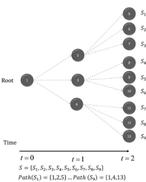
This multistage formulation (shown in Figure 1) is a straightforward extension of the two-stage scenario formulation.
Note that t = 1 represents first-stage decisions, t = 2 represents second-stage decisions and t = 3 represents third-stage decisions.
, , , 1, , ,
i t k BF i t k BF
inl ∈ =in − ∈ ∀ ∈ ∀ ∈ ∀ ∈i L t T k BF (10)
, , , 1, , ,
i t k i t k
inl ≥in − ∀ ∈ ∀ ∈ ∀ ∈i L t T k K (11)
{ }
, , 0;1
i k t
in ∈ (12)
{ }
, , 0;1
i k t
inl ∈ (13)
, , ,
i j p t
xpξ ∈R+ (14)
, , ,
i j p t
xsξ ∈R+ (15)
All parameters used are the same as those seen, with the exception of xpξ
i,j,p and xsi,j,pξ , which
now do not need the index t. Instead of t, the scenario tree precedence is established by the parameter PEξ. Table 1 shows the example used
in our computations.
The uncertainty regarding future events in multistage stochastic programming is modeled through scenarios ξ, and decisions, as in real life, are made at certain points in time t, denominated as stages. The first stage consists of finding warehouse locations to be used at t = 1 and t = 2. Thus, decisions such as where warehouses should be located are made at t = 0. Decisions regarding the quantity of
Notations: Sets and indexes
f ∈ F Distance range
i,j,l ∈ L Cities
k ∈ K Facility type
p ∈ P Product
ξ∈ Ω Scenarios
Subsets
BF ⊂ L Cities that can be selected to have a ixed base PC ⊂ L Cities that can be selected to have a procurement point
U ⊂ L City where the power plant is located Parameters
CCi Loading costs (BRL /ton)
CIi,k Installation costs (BRL)
CMAi,k Maximum facility capacity (ton)
COR Correction factor for secondary transport
CTPp Primary transport costs (BRL/ton.km) CTSf,p Secondary transport costs (BRL/ton) DIi,j Cities distance (km)
LD Distance limit (km)
LFf Range limits (km)
PRξ Scenario probability
PEξ Scenario precedence
PROξi,p P roduction (ton)
Variables
xpξ
i,j,p Amount of castor transported by primary transportation
xsi,j,pξ Amount of castor transported by secondary transportation inξ
i,k Assembled/Built facility
inlξ
i,k Auxiliary facility variable
Table 1. Example of precedence for a tree-stage tree.
ξ Precedence
1 0
2 0
3 0
1.1 1
1.2 1
1.3 1
2.1 2
2.2 2
2.3 2
3.1 3
3.2 3
3.3 3
castor seed flow among cities are made in periods t = 1 and t = 2. The calculated flow is affected by the warehouse locations defined at t = 0. Moreover, this model allows some of the decisions made at period t = 0 to be changed. Depending on the performance of the first harvest, which is known after period t = 0, some procurement points can be disassembled.
The variable ini,kξ ∈ PC is used for both t = 0 and t = 1 stages. In this case, the model can choose to review procurement point assembly decisions. Variable inξ
i,k∈ BF is the decision variable, which remains
unchanged from the first stage to the third stage. Variables xpi,j,pξ and xsi,j,p ξ are second- and third-stage variables, respectively. The mathematical model can be stated as follows:
Objective function
Min Z=pin+ptr+pca (16)
(
)
, , , , ,
i k i k i k i k
pin= ξCI inξ∑ inlξ (17)−
, , , , , , , , , , , , , , ,
i j p f i j p i j p i j p f i j f p i j p
ptr= ∑ ξ PR DI CTP xpξ ξ + ∑ ξ PR DI CTSξ xsξ (18)
, , , , , , , , , ,
i j p i i j p i j p i i j p
pca∑ = ξPR CC xpξ ξ +COR∑ ξPR CC xsξ ξ (19)
The objective function (16) is compounded by three distinct costs, which are defined by terms (17), (18) and (19). Term (17) shows the warehouse installation cost, term (18) is the transportation costs, and term (19) is the loading/unloading truck operation cost. Installation costs occur at
the first and second stages, whereas transportation and loading/unloading costs occur at the second and third stages. The term inξ
i,k – inl
ξ
i,k, as in the
two-stage model, is created to guarantee that the installation cost occurs only when a facility is installed.
, 1 ,
kini kξ i L ξ
∑ ≤ ∀ ∈ ∀ ∈Ω (20)
, , , , , , ,
PE
j pxsi j p kCMA ini k i k i j L
ξ ξ
∑ ≤ ∑ ∀ ∈ ∀ ξ ∈Ω (21)
(
, , , ,)
,(
, , , ,)
, , , ,i xpi j pξ xsi j pξ PROξj p l xpξj l p xsξj l p i j l L p P
∑ + + ≤ ∑ + ∀ ∈ ∀ ∈ ∀ ξ ∈Ω (22)
(
)
{ }| , , , , , , , , , ( 0 )
i i U∉ PROi pξ i uξ xpi u pξ xsi u pξ p P
∑ ≤ ∑ + ∀ ∈ ∀ ξ ∈ Ω − (23)
, 0, ,
i k PC
inlξ∈ = ∀ ∈ ∀ ξ ∈Ωi L (24)
î
,
, , ,
PE i k BF i k BF
inlξ∈ =in ∈ ∀ ∈ ∀ ξ ∈Ωi L (25)
{ }
, 0;1 , , ,
i k
inξ ∈ ∀ ∈ ∀ ξ ∈Ω ∀ ∈i L k K (26)
{ }
, 0;1 , , ,
i k
inlξ ∈ ∀ ∈ ∀ ξ ∈Ω ∀ ∈i L k K (27)
, , , , , ,
i j p
xpξ ∈R+∀i j∈ ∀ ξ ∈Ω ∀ ∈L p P (28)
, , , , , , , ,
i j p t
Constraint (20) limits to one the number of facilities that can be installed in each city. Constraint (21) defines warehouse storage capacity and ensures that castor seed transportation is executed only if a warehouse has been previously installed. In (22), a flow balance constraint indicates that the total production transported to warehouses must be equal to the total production of the producers. Constraint (23) guarantees that the amounts of castor seeds produced and delivered to a plant are equal (another flow balance constraint). In (24), a constraint sets the value for inlξ
i,k∈ PC. This variable
is set equal to 0 due to procurement costs, which occur at each period. (25) is a nonanticipativity constraint that ensures that any decision made for the fixed bases in period t -1 remains unchanged in period t. When we split the scenarios, we may have lost the nonanticipativity of the decisions because such decisions would now include knowledge of the outcomes up to the end of the horizon. To enforce nonanticipativity, we add constraints explicitly in the formulation (Birge & Louveaux, 1997). These nonanticipativity constraints are the only constraints linking the separate scenarios. Without them, the problem would decompose into a separate problem for each ξ, maintaining the structure of that problem (Birge & Louveaux, 1997). (26)-(29) are similar to the two-stage model.
4. Case study
The case study involves an area located in a poor and semi-arid region in Brazil that is primarily populated by small farmers. Many of these farmers produce castor seeds. The Brazilian government has set this region of the country as one of its priorities to improve the quality of life by promoting prosperity. To achieve these goals, the Brazilian government has focused on including diligently these small farmers in the Brazilian Biodiesel Program (BBP). According to Leão et al. (2011), the majority of the people who live in this area have poor education levels compared with other areas in Brazil. This population also has low income, lacks a basic sewer infrastructure, and does not have access to a decent healthcare system. Brazil’s semi-arid region covers eight of the nine states in the Northeast region and includes the
northern Minas Gerais state, representing an area of approximately 1.0 million square kilometers.
Castor seed was selected as one of the main oilseed sources for biodiesel production due to its inherent properties, such as hardiness, capability to survive in severe weather conditions, and good adaptation to intercropping (Leão et al., 2011). Furthermore, the castor seed production techniques are well known and widespread among farmers in the region, which also contributed to castor seed being selected as an important source for the PNPB (Leão et al., 2011). These small farmers live in rural areas, usually far from medium and large cities. Therefore, to sell their castor seed production, the farmers are obligated to transport their production to different locations where a fixed base or procurement point can be found. Thus, the central issue concerns finding suitable locations for these facilities to then ship the whole production to the plant. The challenge involves minimizing both the installation of facilities and the transportation costs.
The production level varies according to the weather conditions, i.e., the amount of rainfall. There is always uncertainty associated with the production. Rainfall may largely affect the whole logistics network efficiency, which may have to be redesigned depending on the production levels. At this point, some important questions emerge, e.g., how will the logistics network be designed/redesigned, considering such uncertainty? The stochastic modeling approach can therefore support the design of the Brazilian biodiesel supply chain.
5. Results and discussion
This section shows the main results found for the two- and multistage models and the scenario generation considerations. All calculations were conducted using a system that generated scenarios via a VBA (Visual Basic for Applications) script. VBA
routines also connected the generated scenarios to a database stored in MS Access. Then, the data were automatically sent to AIMMS for the mathematical
model, and the results were compiled in MS Excel. Figure 2 shows our system.
5.1. Scenario generation
A crucial part of any stochastic program study is generating scenarios that fairly represent uncertainties to obtain accurate results. The importance of this subject has been noted by Date et al. (2008), Falasca & Zobel (2011), and Balibek & Koksalan (2012). The issue of representing uncertainties through quantitative models is complex and well known (Hoyland & Wallace, 2001). One of the main challenges is to collect data from the limited available production data set. The lack of historical production data for each candidate city was an issue. To overcome it, the proposed approach utilized the percentage of national production deviations, which includes outputs for several counties in Brazil (Companhia Nacional de Abastecimento, 2012). The percentage deviations are plotted in Figure 3 (Y-Axis). There are 35 periods (X-Axis). The first period is the difference in crop production between 1976-77 and 1978-79, the second period is the difference between 1980-81 and 1982-83, and so on. Figure 2 shows the percentage deviations.
Given the limited amount of data available with respect to the castor crops, it would be more reliable to use a discretization method that can select three appropriate points to represent the distribution of the percentage deviations. Therefore, the next step is to plot a cumulative distribution histogram, as shown in Figure 4.
According to Hoyland & Wallace (2001), one method of generating scenarios consists of finding
a simple discrete approximation. The approximation works as the initial input to the model. Keefer
& Bodily (1983) proposed an extension of the Swanson-Megill method. The authors suggested an Extended Swanson-Megill, where the 10%, 50% and 90% percentiles are weighted by the probabilities 0.3, 0.4 and 0.3, resulting in corresponding values of -59.38%, -2.78% and 104.39%.
5.2. Two-stage results and discussion
The S2OS model was built on the AIMMS
3.14 platform and has a total of 5,488 constraints and 28,204 variables, with a solution time of approximately 5 seconds using an Intel Core i5 – 421OU CPU 2.4 GHz with 4.0 GB of RAM memory. The solver used was CPLEX 12.5. Thus, this problem is not considered a problem that would generate computational problems, and we can conclude that a real-world two-stage model of such an instance can be quickly solved and provide sufficiently fast solutions for decisions made on a daily basis.
We measure the quality of the stochastic two-stage optimization model (S2SO model) solution using VSS. which consists of the difference between the expected result of using the expected value solution (EEV), which was 9,156,309.01 (BRL), and the Recourse Problem (RP), which was 8,628,002.77 (BRL). Thus, we find a Value of Stochastic Solution: VSS = EEV - RP = 605,547.46. We can affirm that the decision makers would have savings of 605,547.46,
representing 6.61% of EEV, when uncertainty is incorporated into the model. In terms of facilities, it means positioning a facility at t - 1 in the city of Independência (CE), which is responsible for various flow changes in the region. EVPI is calculated using WS (Wait-and-see), which in practice indicates the possibility to calculate the optimization with the absolute certainty of occurrence of a specific production scenario. The value found for WS was 8,550,761.55; thus, |WS - RP | = 77,241.22, being 0.90% of RP. This low value means that for this specific scenario tree, there is not much financial gain in using perfect information.
5.3 Multistage results and discussion
This section presents the main findings based on the proposed multistage model for small farmers. The three-stage model was built on the AIMMS 3.14 platform. It has 4,529 constraints and a total of 19,246 variables. The computation time required to solve the case study on a typical desktop computer was less than 10 seconds using the CPLEX 12.5 solver, using an Intel Core i5 – 421OU CPU 2.4 GHz with 4.0 GB of RAM memory. The solver used was CPLEX 12.5. As for the two-stage model, this problem also cannot be considered a great instance problem
that could generate computational problems, and we can conclude that a real-world three-stage model of such an instance can also be quickly solved and provide sufficiently fast solutions for the decisions made on a daily basis.
The results obtained using the Stochastic 3 Stage Optimization (S3SO) model are compared with those of the S2SO approach. The optimal cost obtained by S3SO was 7,700,019 (BRL). The optimal cost obtained by S2SO was 8,628,002 (BRL), resulting in a savings of 927,983 (BRL). Table 2 shows where the procurement points and fixed base facilities should be located and their quantities, as calculated using S3SO and S2SO.
A gain of 10.75% is obtained when S3SO is applied to the Brazilian biodiesel supply chain design. This gain is obtained due to the flexibility in S3SO. It represents a huge impact on the rural area in Brazil, where a reduction in costs can benefit several small farmers and the whole Brazilian biodiesel supply chain program (Programa Nacional de Produção de Biodiesel, 2013). Table 2 summarizes the main results.
Table 3 shows the summary of the main indicators: using the S3SO model, at t = 1, the facility in
Juru (PB) was disassembled. S2SO does not have this capability; therefore, Juru (PB) continued to have an unnecessary facility at t = 1. Nagar & Jain (2008) used a measure of performance called Gain of Added Flexibility (GAF), which was applied in this work to measure the difference between the S2SO and S3SO results. The GAF is simply calculated by using the costs obtained using S2SO and S3SO as follows: GAF = S2SO - S3SO = R$927,983, which is 10.75% of the S2SO solution.
Table 2. Main results.
City Facility
S3SO S2SO
Period and Scenarios Period
t=0 t=1 t=0 t=1
0 1 2 3
Boa Viagem (CE) Procurement Point 1
Caracol (PI) Procurement Point 1 1 1 1 1 1
Catunda (CE) Procurement Point 1 1 1 1 1 1
Independência (CE) Procurement Point 1 1 1 1
Itatira (CE) Procurement Point 1 1 1 1 1 1
Juru (PB) Procurement Point 1 1 1
Matias Cardoso (MG) Fixed Base 1 1 1 1 1 1
Mombaça (CE) Procurement Point 1 1 1
Mossoró (RN) Procurement Point 1
Nova Redenção (BA) Fixed Base 1 1 1 1 1 1
Ouricuri (PE) Procurement Point 1 1 1 1 1 1
Pedra Branca (CE) Procurement Point 1 1 1 1 1 1
Pilão Arcado (BA) Procurement Point 1 1 1
Porteirinha (MG) Procurement Point 1 1 1 1 1 1
Quixadá (CE) Fixed Base 1 1 1 1 1 1
Remígio (PB) Procurement Point 1 1 1 1 1 1
Santa Cruz (RN) Procurement Point 1 1 1 1 1 1
São Francisco (MG) Procurement Point 1 1 1 1
Serra do Ramalho (BA) Fixed Base 1 1 1 1 1 1
Serra Talhada (PE) Procurement Point 1 1 1 1 1 1
Tamboril (CE) Procurement Point 1
Tauá (CE) Fixed Base 1 1 1 1 1 1
Irecê (BA) Fixed Base 1 1 1 1 1 1
S3SO Total Procurement Points 13 9 14 17
Total Fixed Bases 6 6 6 6
S2SO Total Procurement Points 11 12
Total Fixed Bases 6 6
Source: elaborated by the authors (2016).
Table 3. Summary of main indicators.
Model Objective Function Indicator Absolute Value Dif (%) Value
EEV R$ 605,55 VSS R$ 605.547 VSS/EEV 6.61%
WS R$ 8,550,761 EVPI R$ 77.241 EVPI/SO2S 0.90%
SO2S R$ 9,156,309 GAF R$ 927,983 GAF/SO2S 10.75%
SO3S R$ 7,700,019
Companhia Nacional de Abastecimento. (2012). Brasília: CONAB. Retrieved in 23 September 2015, from http:// www.conab.gov.br
Dantzig, G. (1955). Linear programming under uncertainty. Management Science, 50(12), 1764-1769.
Date, P., Mamon, R., & Jalen, L. (2008). A new moment matching algorithm for sampling from partially specified symmetric distributions. Operations Research Letters, 36(6), 669-672. http://dx.doi.org/10.1016/j.orl.2008.07.004.
Demirbas, M., & Balat, M. (2006). Recent advances on the production and utilization trends of bio-fuels: a global perspective. Energy Conversion and Management, 47(15-16), 2371-2381. http://dx.doi.org/10.1016/j.enconman.2005.11.014. Falasca, M., & Zobel, C. W. (2011). A two-stage procurement
model for humanitarian relief supply chains. Journal of Humanitarian Logistics and Supply Chain Management., 1(2), 151-169. http://dx.doi.org/10.1108/20426741111188329. Haas, M. J., Mcaloon, A. J., Yee, W. C., & Foglia, T. A. (2006).
A process model to estimate biodiesel production costs. Bioresource Technology, 97(4), 671-678. http://dx.doi. org/10.1016/j.biortech.2005.03.039. PMid:15935657. Haneveld, W. K. K., & Vlerk, M. H. V. D. (1999). Stochastic
integer programming: general models and algorithms. Annals of Operations Research, 85, 39-57. http://dx.doi. org/10.1023/A:1018930113099.
Hoffman, J., & Schniederjans, M. (1994). A two-stage model for structuring global facility site selection decisions. International Journal of Operations & Production Management, 14(4), 79-96. http://dx.doi.org/10.1108/01443579410056065. Hoyland, K., & Wallace, S. W. (2001). Generating Scenario Trees
for Multistage decision problems. Management Science, 47(2), 295-307. http://dx.doi.org/10.1287/mnsc.47.2.295.9834. Jayaraman, V. (1998). An efcient heuristic procedure for practical-sized capacitated warehouse design and management. Decision Sciences Journal., 29(3), 729-745. http://dx.doi. org/10.1111/j.1540-5915.1998.tb01361.x.
Kaut, M., & Wallace, S. W. (2007). Evaluation of scenario generation methods for stochastic programming. Pacific Journal of Optimization, 3(2), 257-271.
Keefer, D. L., & Bodily, S. E. (1983). Three-point approximations for continuous random variables. Management Science, 29(5), 595-609. http://dx.doi.org/10.1287/mnsc.29.5.595. Leão, R. R. C. C., Hamacher, S., & Oliveira, F. (2011). Optimization
of biodiesel supply chains based on small farmers: a case study in Brazil. Bioresource Technology, 102(19), 8958-8963. http://dx.doi.org/10.1016/j.biortech.2011.07.002. PMid:21816610.
Leduc, S., Natarajan, K., Dotzauer, E., Mccallum, I., & Obersteiner, M. (2009). Optimizing biodiesel production in India. Applied Energy, 86(1), S125-S131. http://dx.doi.org/10.1016/j. apenergy.2009.05.024.
Lee, J. H. (2014). Energy supply planning and supply chain optimization under uncertainty. Journal of Process Control, 24(2), 323-331. http://dx.doi.org/10.1016/j. jprocont.2013.09.025.
Messina, E. & Mitra, G. (1997). Modelling and analysis of multistage stochastic programming problems: a software environment. European Journal of Operations Research, 101, 343-359.
Nagar, L., & Jain, K. (2008). Supply chain planning using multi-stage stochastic programming. Supply Chain Management:
6. Conclusions
This paper addressed a real-life problem that is central to developing a sustainable program for biodiesel use and production in Brazil. Moreover, the Brazilian government seeks to promote prosperity among small farmers by including their production in the biodiesel supply chain. Several models can be found in the literature that minimize the total cost of the supply chain. As found in the work of Nagar
& Jain (2008), the proposed multi-stage model is compared with the standard two-stage model by examining the difference between the objective values of two solutions. Nagar and Jain considered a percentage savings of 5.43% to be good savings; thus, our 10.75% percentage savings can also be considered good savings.
To generate the scenarios, we used the discretization method Extended Swanson-Megill. The performance of the stochastic programming model depends directly on the scenario tree that is generated to represent uncertainty. There were not sufficient data to assess the real probability distribution of castor.
The real world problem had a small instance that considered real-life optimization models. Nevertheless, a natural extension of this paper could consider increasing the instance and applying solution methods such as the L-Shaped Method, which is a stochastic form of Benders Decomposition. Other approaches for uncertainty, such as Fuzzy sets and Robust optimization, could be tested and compared.
References
Ahmed, S., King, A. J., & Parija, G. (2003). A multi-stage stochastic integer programming approach for capacity expansion under uncertainty. Journal of Global Optimization, 26(1), 3-24. http://dx.doi.org/10.1023/A:1023062915106. Balibek, E., & Koksalan, M. (2012). A visual interactive approach
for scenario-based stochastic multi-objective problems and an application. The Journal of the Operational Research Society, 63(12), 1773-1787. http://dx.doi.org/10.1057/ jors.2012.25.
Beraldi, P., Musmanno, R., & Triki, C. (2000). Solving stochastic linear programs with restricted recourse using interior point methods. Computational Optimization and Applications, 15(3), 215-234. http://dx.doi.org/10.1023/A:1008772217145. Birge, J. R., & Louveaux, F. (1997). Introduction to stochastic
programming (Springer Series in Operations Research). New York: Springer-Verlag.
Carraretto, C., Macor, A., Mirandola, A., Stoppato, A., & Tonon, S. (2004). Biodiesel as alternative fuel: experimental analysis and energetic evaluations. Energy, 29(12-15), 2195-2211. http://dx.doi.org/10.1016/j.energy.2004.03.042. Casey, M. S., & Sen, S. (2005). The scenario generation algorithm
Sotoft, L. F., Rong, B., Christensen, K. V., & Norddahl, B. (2010). Process simulation and economical evaluation of enzymatic biodiesel production plant. Bioresource Technology, 101(14), 5266-5274. http://dx.doi.org/10.1016/j. biortech.2010.01.130. PMid:20171880.
Van Dyne, D. L., Weber, J. A., & Braschler, C. H. (1996). Macroeconomic effects of a community-based biodiesel production system. Bioresource Technology, 56(1), 1-6. http://dx.doi.org/10.1016/0960-8524(95)00173-5. Xie, F., Huang, Y., & Eksioglu, S. (2014). Integrating multimodal
transport into cellulosic biofuel supply chain design under feedstock seasonality with a case study based on California. Bioresource Technology, 152, 15-23. http:// dx.doi.org/10.1016/j.biortech.2013.10.074. PMid:24275021. Zhang, M., Huang, J., & Zhu, J. (2012). Reliable facility location
problem considering facility failure scenarios. Kybernetes, 41(10), 1440-1461. http://dx.doi.org/10.1108/03684921211276666. Zhang, Y., Dube, M. A., Mclean, D. D., & Kates, M. (2003). Biodiesel
production from waste cooking oil: 1. Process design and technological assessment. Bioresource Technology, 89(1), 1-16. http://dx.doi.org/10.1016/S0960-8524(03)00040-3. PMid:12676496.
Acknowledgements
The authors would like to thank the two anonymous referees for their valuable comments, which greatly improved the quality of this paper.
An International Journal., 13(3), 251-256. http://dx.doi. org/10.1108/13598540810871299.
Oliveira, F., & Hamacher, S. (2012). A simulation-based approach to the optimization of the petroleum product supply chain under uncertainty: a case study in northern Brazil. Industrial & Engineering Chemistry Research, 51(11), 4279-4287. http://dx.doi.org/10.1021/ie2013339.
Programa Nacional de Produção de Biodiesel. (2013). Retrieved in 23 September 2015, from http://portal.mda.gov.br/ portal/saf/programas/biodiesel/2286217
Ribas, G. P. (2008). Modelo de programação estocástica para o planejamento estratégico da cadeia integrada de petróleo (Dissertação de mestrado). Pontifícia Universidade Católica do Rio de Janeiro, Rio de Janeiro.
Riis, M., & Andersen, K. A. (2005). Applying the minimax criterion in stochastic recourse programs. European Journal of Operational Research, 165(3), 569-584. http://dx.doi. org/10.1016/j.ejor.2003.09.033.
Sahinidis, N. (2004). Optimization under uncertainty: state-of-the-art and opportunities. Computers and Chemical Engineering, 28(6-7), 971-983.
Table 4A. Estimated production.
States Production (μ ton)
BA 748.69
CE 2,235.79
MG 545.65
PB 112.41
PE 796.71
PI 85.91
RN 112.72
Total 4,636.90
Appendix A. Data used in calculations. Table 1A. Model nodes.
Elements Total
Cities 145
Plants 1
Possible Procurement points 26
Possible fixed bases 9
Table 2A. Loading costs: multiplied by κ to preserve confidentiality.
Type of transportation Loading costs (κBRL/ton)
Primary 2
Secondary 1
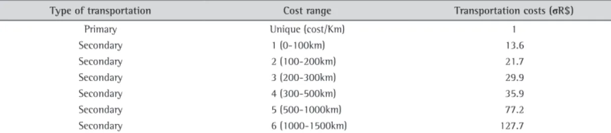
Table 3A. Transportation costs: multiplied by σ to preserve confidentiality.
Type of transportation Cost range Transportation costs (σR$)
Primary Unique (cost/Km) 1
Secondary 1 (0-100km) 13.6
Secondary 2 (100-200km) 21.7
Secondary 3 (200-300km) 29.9
Secondary 4 (300-500km) 35.9
Secondary 5 (500-1000km) 77.2
Secondary 6 (1000-1500km) 127.7
Table 5A. Facility capacity.
Facility Capacity (ton)
Procurement point 4500