A Study of the Protein Folding Dynamic
Omar GACI
∗Abstract—In this paper, we propose two means to study the protein folding dynamic. We rely on the HP model to study the protein folding problem in a con-tinuous graphic environment. The amino acids evolve according to the boid rules, we observe a collective behavior due to the attraction between residues of H type. We propose a first step to simulate a folding process. As well, we present a way to fold a protein when it is represented by an amino acid interaction network. This is a graph whose vertices are the pro-teins amino acids and whose edges are the interactions between them. We propose a genetic algorithm of reconstructing the graph of interactions between sec-ondary structure elements which describe the struc-tural motifs. The performance of our algorithms is validated experimentally.
Keywords: boids, protein folding problem, interaction networks, genetic algorithm
1
Introduction
Proteins are biological macromolecules participating in the large majority of processes which govern organisms. The roles played by proteins are varied and complex. Certain proteins, called enzymes, act as catalysts and increase several orders of magnitude, with a remarkable specificity, the speed of multiple chemical reactions essen-tial to the organism survival. Proteins are also used for storage and transport of small molecules or ions, control the passage of molecules through the cell membranes, etc. Hormones, which transmit information and allow the reg-ulation of complex cellular processes, are also proteins.
Genome sequencing projects generate an ever increasing number of protein sequences. For example, the Human Genome Project has identified over 30,000 genes which may encode about 100,000 proteins. One of the first tasks when annotating a new genome, is to assign functions to the proteins produced by the genes. To fully understand the biological functions of proteins, the knowledge of their structure is essential.
In their natural environment, proteins adopt a native compact three-dimensional form. This process is called folding and is not fully understood. The process is a result of interactions between the protein’s amino acids
∗Le Havre University, LITIS Laboratory - EA 4108, Le Havre
76600 France Fax: +33 232 744 382 Email: [email protected]
which form chemical bonds.
In this study, we propose two means to study the pro-tein folding problem. First, we treat propro-teins as chains where the amino acids are identified by their hydropho-bicity according to the HP model [?]. Then, we consider that a residue is an individual which evolves with a boid behavior. A boid behavior is notably characterized by three rules which ensure that a population of individuals stays grouped when it is in movement. We carry out a study to develop a JAVA application where the confor-mational space is represented by a 3D continuous graph-ical environment. Thus, a protein is a sequence whose amino acids will evolve as boid. The goal is to fold this protein to give a new graphical interpretation of the HP model. Second, we treat proteins as networks of interact-ing amino acid pairs [3]. In particular, we consider the subgraph induced by the set of amino acids participating in the secondary structure also called Secondary Struc-ture Elements (SSE). We call this graph SSE interaction network (SSE-IN). We begin by recapitulating relative works about this kind of study model. Then, we present a genetic algorithm able to reconstruct the graph whose vertices represent the SSE and edges represent spatial in-teractions between them. In other words, this graph is another way to describe the motifs involved in the protein secondary structures.
2
Protein structure
Unlike other biological macromolecules (e.g., DNA), pro-teins have complex, irregular structures. They are built up by amino acids that are linked by peptide bonds to form a polypeptide chain. We distinguish four levels of protein structure:
• The amino acid sequence of a protein’s polypeptide
chain is called its primary or one-dimensional (1D) structure. It can be considered as a word over the 20-letter amino acid alphabet.
• Different elements of the sequence form local regular
secondary (2D) structures, such as α-helices or β -strands.
• The tertiary (3D) structure is formed by packing
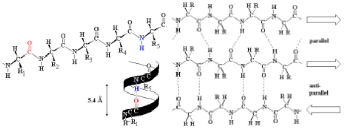
Figure 1: Left: an α-helix illustrated as ribbon diagram, there are 3.6 residues per turn corresponding to 5.4 ˚A. Right: A β-sheet composed by three strands.
• The final protein may contain several polypeptide
chains arranged in a quaternary structure.
By formation of such tertiary and quaternary structure, amino acids far apart in the sequence are brought close together to form functional regions (active sites). The reader can find more on protein structure in [6].
One of the general principles of protein structure is that hydrophobic residues prefer to be inside the protein con-tributing to form a hydrophobic core and a hydrophilic surface. To maintain a high residue density in the hy-drophobic core, proteins adopt regular secondary struc-tures that allow non covalent hydrogen-bond and hold a rigid and stable framework. There are two main classes of secondary structure elements (SSE), α-helices and β -sheets (see Fig. 1).
An α-helix adopts a right-handed helical conformation with 3.6 residues per turn with hydrogen bonds between C’=O group of residuenand NH group of residuen+ 4.
A β-sheet is build up from a combination of several re-gions of the polypeptide chain where hydrogen bonds can form between C’=O groups of oneβ strand and another NH group parallel to the first strand. There are two kinds ofβ-sheet formations, anti-parallelβ-sheets (in which the two strands run in opposite directions) and parallel sheets (in which the two strands run in the same direction).
Based on the local organization of the secondary struc-ture elements (SSE), proteins are divided in the following four classes [17]:
• All α, proteins have only α-helix secondary
struc-ture.
• Allβ, proteins have onlyβ-strand secondary
struc-ture.
• α/β, proteins have mixedα-helix andβ-strand
sec-ondary structure.
• α+β, proteins have separatedα-helix andβ-strand
secondary structure.
From this first division, a more detailed classification can be done. The most frequently used ones are SCOP, Struc-tural Classification Of Proteins [20], and CATH, Class Architecture Topology Homology [21]. They are hierar-chical classifications of proteins’ structural domains. A domain corresponds to a part of a protein which has a hydrophobic core and not much interaction with other parts of the protein.
3
The Protein Folding Problem
Several tens of thousands of protein sequences are en-coded in the human genome. A protein is comparable to an amino acid chain which folds to adopt its tertiary structure. Thus, this 3D structure enables a protein to achieve its biological function. In vivo, each protein must quickly find its native structure, functional, among innu-merable alternative conformations.
The protein 3D structure prediction is one of the most important problems of bioinformatics and remains how-ever still irresolute in the majority of cases. The problem is summarized by the following question: being given a protein defined by its sequence of amino acids, which is its native structure?, i.e., the structure whose amino acids are correctly organized in three dimensions so that pro-teins can achieve correctly their biological functions. As well, the native structure is considered as the most stable with a minimum energy level.
Unfortunately, the exact answer is not always possible that is why the researchers have developed study models to provide a feasible solution for any unknown sequences. However, models to fold proteins bring back to NP-Hard optimization problems [8]. Those kinds of models con-sider a conformational space where the modeled protein tries to reach its minimum energy level which corresponds to its native structure.
Therefore, any algorithm of resolution seems improbable and ineffective, the fact is that in the absolute no study model is yet able to entirely define the general principles of the protein folding.
3.1
The Levinthal Paradox
The first observation of spontaneous and reversible fold-ingin vitro was carried out by Anfinsen [1]. He deduced that the native structure of a protein corresponds to a conformation with a minimal free energy, at least un-der suitable environmental conditions. But if the protein folding is indeed under thermodynamic control, a judi-cious question is to know how a protein can find, in a reasonable time, its structure of lower energy among an astronomical number of possible conformations.
As example, a protein of 100 residues can adopt 2100 (≃
1030
two possibilities are accessible to each residue. If the passage from a conformation to another is carried out in 10−13seconds (which corresponds to time necessary for a
rotation around a connection), this protein would need at least 1017
seconds, i.e. approximately three billion years, ”to test” all possible conformations. The proteins how-ever manage to find their native structures in a lapse of time which is about the millisecond at the second. The apparent incompatibility between these facts, raised ini-tially by Levinthal in [16], was quickly set up in paradox and made run enormously ink since.
Levinthal gives the solution of its paradox: proteins do not explore the totality of their conformational space, and their folding needs to be ”guided”, for example via the fast formation of certain interactions which would be determining for the continuation of the process.
3.2
Motivations
To be able to understand how a protein accomplishes its biological function, and to be able to act on the cellular processes in which the protein intervenes, it is essential to know its structure. Many protein native structures were determined experimentally - primarily by crystallography with Xrays or by Nuclear Magnetic Resonance (NMR) -and indexed in a database accessible to all, Protein Data Bank (PDB) [5].
However, the application of these experimental tech-niques consumes a considerable time [15, 22]. Indeed, the number of protein sequences known [4] is much more important than the number of solved structures [5], this gap continues to grow quickly.
The design of methods making it possible to predict the protein structure from its sequence is a problem whose stakes are major, and which fascinate many of scientists for several decades. Various tracks were followed with an aim of solving this problem, elementary in theory but extremely complex in practice.
4
Simulation Models
In this section we present two simulations model from which we present in the next section an application to fold proteins when we know only their sequences.
4.1
The HP Model
One of the most widespread models for the protein folding study is the HP model, hydrophobic-hydrophilic. The term HP-Model was presented by Dill [?] to indicate a grid model on two dimensions with an energy function which is simplified as much as possible.
Proteins are chains of monomers whose each one is a va-riety of the 20 natural amino acids. In the HP model, only two types of monomers are exploited: those said
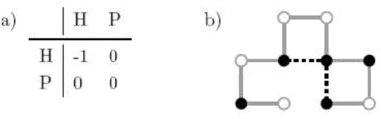
Figure 2: A description of the HP model. (a) Energy matrix, the no covalent interactions between amino acids of H type reduce the current energy level. (b) An example of conformation with the HP model. The black nodes are hydrophobic, they are of H type.
hydrophobic (H), which tend to aggregate each others to prevent from being surrounded by water and those known as polar or hydrophilic (P), which are attracted by wa-ter and are often found in the folding border. Thus, the nodes of the H type are supposed to attract each other while the P nodes are neutral.
The energy function is given by the Fig. 2 and is such as the energy contribution of a no covalent contact between two monomers is -1 if the two residues are of H type, and 0 differently. A no covalent contact between two monomers is definite if their Euclidean distance is worth a unit and if they are not associated by a physical bond. A conformation with a minimal energy corresponds to a folding with a maximum no covalent number of con-tacts between monomers of H type. The native structure prediction problem via the HP model was shown to be NP-Hard problem [8].
A specific conformation of the sequence PHPHPPHHPH with an energy level is -2 is given Fig. 2. The white pearls represent the amino acids of P type and the blacks those of H type. The two contacts indicated in dotted line are no covalent contacts and allow to evaluate the global energy of the system.
4.2
The Amino Acid Interaction Network
The 3D structure of a protein is represented by the coor-dinates of its atoms. This information is available in Pro-tein Data Bank (PDB) [5], which regroups all experimen-tally solved protein structures. Using the coordinates of two atoms, one can compute the distance between them. We define the distance between two amino acids as the distance between their Cα atoms. Considering the Cα atom as a “center” of the amino acid is an approxima-tion, but it works well enough for our purposes. Let us denote by N the number of amino acids in the protein. A contact map matrix is a N×N 0-1 matrix, whose
β-sheets appear as bands parallel or perpendicular to the main diagonal [14]. There are different ways to define the contact between two amino acids. Our notion is based on spacial proximity, so that the contact map can consider non-covalent interactions. We say that two amino acids are in contact if and only if the distance between them is below a given threshold. A commonly used threshold is 7 ˚A [3] and this is the value we use.
Consider a graph with N vertices (each vertex corre-sponds to an amino acid) and the contact map matrix as incidence matrix. It is called contact map graph. The contact map graph is an abstract description of the pro-tein structure taking into account only the interactions between the amino acids.
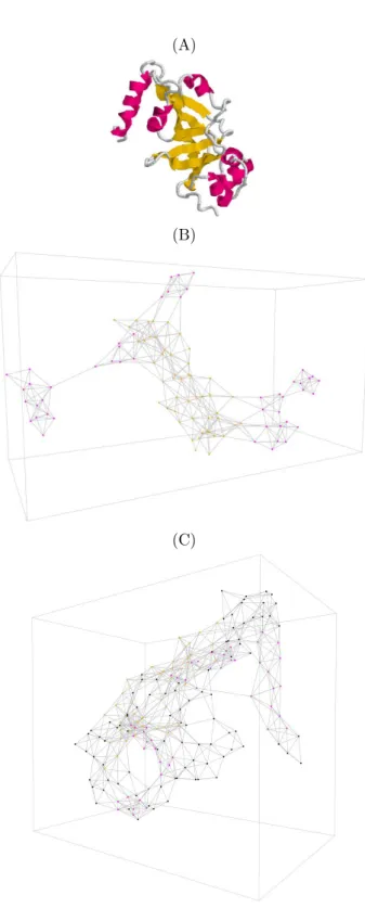
First, we consider the graph induced by the entire set of amino acids participating in folded proteins. We call this graph the three dimensional structure elements interac-tion network (3DSE-IN), see Fig. 3-C.
As well, we consider the subgraph induced by the set of amino acids participating in SSE. We call this graph SSE interaction network (SSE-IN), see Fig. 3-B.
To manipulate a SSE-IN or a 3DSE-IN, we need a PDB file which is transformed by a parser we have developed. This parser generates a new file which is read by the GraphStream library to display the SSE-IN in two or three dimensions.
5
A Simulation Model Based on the
Boids Behavior
Our goal is to exploit the HP model to propose a means to simulate the folding process. Here, the amino acids are boids and evolve as a consequence.
The alphabet of 20 amino acids letters is reduced to two letters, namely H and P. The residues of the H type represent hydrophobic amino acids, whereas those of P type are polar and are the hydrophilic amino acids. In the same way, the energy function checks the illustration given in Fig. 2, the goal being to maximize no covalent contacts of H-H type to minimize the global energy of the modeled protein.
5.1
A Boid Behaviour
The observation of birds clouds, in which one or more thousands of birds fly in a mass which seems compact, becoming deformed, being divided sometimes into sev-eral swarms, then being reformed given birth to some interrogations. The single character of the bird masses is the first character which strikes imagination. We can also be astonished by the significant number of animals within the clouds, and their capacity, however, to avoid each others. Such clouds seem ”directed”, by a collective direction.
(A)
(B)
(C)
Figure 4: The three boid behavioral constraints. A boid has a radius of perception represented as a circle to de-termine its neighborhood. A boid adapts its velocity as a function of its neighbors.
One of the first researchers who studied this subject un-der the angle of the cloud phenomena modeling is Craig Reynolds [23]. The solution suggested is astonishing of simplicity, and gives a particularly faithful model of the bird clouds, fish benches, etc.
The model is based on a personal representation, each in-dividual is modeled explicitly with simple behavior rules. Each boid flies according to a direction vector which indi-cates also its velocity. During its motion, a boid respects three constraints, see Fig. 4, which are the following:
• Separation: boids try to avoid the collisions with
their neighbors.
• Alignment: they tend to align their direction vector
and their velocity with their neighbors.
• Cohesion: they move to the barycenter of their
neighbors.
The neighbors of a boid are defined by a vision radius such as shown by Fig. 4 and which is represented by a circle (the angle is 360 degrees).
These simple behavior rules create a collective behavior which particularly looks like the one of birds clouds or fish benches. Obviously, certain rules can be added so that there are various type of boids.
5.2
Adaptations to Fold Proteins
To exploit a boid behavior to fold a sequence, we need to define the groups of amino acids which evolve as boids. Thus, the residues of H type will evolve as boids with a specific cohesion rule.
To apply the Reynolds rules to the residues, in particu-lar the rule of separation, we must exploit an ”elasticity” on the connections. The variation of the bond lengths makes it possible to highlight the mechanisms of attrac-tion involved between hydrophobic residues. Therefore, the length of connections inter amino acids will evolve between a minimum and a maximum length. Then, the bonds become rubber bands whose length is limited. Let us notice here that the bond minimal length returns to consider a mutual repulsion force between two covalent amino acids which are two close.
5.3
Energy Evaluation
The energy function we exploit corresponds to the one described in Fig. 2. The goal is to maximize the num-ber of non-covalent contact, i.e. without physical bonds, between hydrophobic residues.
We consider that if two amino acids of H type evolve in the graphical space with a distance below a certain threshold then we update the energy function adding−1.
When, the folding process is unable to decrease the en-ergy level, we stop the simulation.
5.4
Simulation of a Boid Dynamic
The programming language we choose is Java3D which allows us to apply an object modeling to develop our sim-ulator. The dataset is composed of 20 chains represented through the HP model.
As we have already exposed, we want to reproduce the folding process considering that amino acids are boids. Then, the amino acids of H type tend to regroup each others to act as boids.
The three Reynolds rules will lead the simulation process. The residues will move in the graphical scene accord-ing to their velocity, direction and neighborhood. Ob-viously, the amino acid type, namely hydrophilic (H) or hydrophobic (P), determines which laws will govern the folding. The two types of amino acids will obey mutually to the rules of separation and alignment while the cohe-sion rule will differ to reproduce the attraction between the hydrophobic amino acids. The general principle of our simulations is given by Algorithm 1.
parame-Algorithm 1:Description of the general principle of our simulations to fold a sequence modeled by the HP model with a boid behavior.
Input:
setBoids: all amino acids setH: amino acids of H type Data:
vision: radius of neighborhood perception position: 3D position of a Boid
begin
energy←−0
while energy is decreasingdo foreach b∈setBoids do
P os3D←−position(b)
V1←−separationRule(vision, P os3D) V2←−alignementRule(vision, P os3D) if b∈setH then
V3←−cohesionRule(vision, P os3D) else
V3←−cohesionRule(P os3D) position(b)←−scale(V1, V2, V3)
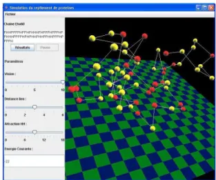
ters. When the native structure is reached, the user will be able to launch the comparison between the folding ob-tained and the one available at the PDB, see Fig. 5.
5.5
Folding Evaluation
Proteins whose native structure is determined are avail-able at PDB. This organization provides files with the three-dimensional coordinates of each protein. Neverthe-less, the coordinates available are expressed in a specific format and it is not possible to compare them to the one obtained from our simulations. Consequently, we apply a transformation to the simulation coordinates to express them in the PDB format. It remains us to draw in the same reference mark, the two structures, see Fig. 6. The score of this superposition is calculated by summing the Euclidean distances between the amino acids of the two structures to obtain a RMSD score.
5.6
Synthesis
The goal of this first application is to propose at the same time a study model for the protein folding and a graphic simulation able to highlight the dynamic of phenomena engaged during the folding process.
The method implemented exploits the hydrophilic and hydrophobic properties of a protein chain modeled ac-cording to the HP model. The motion of elements is governed by the Reynolds laws which make it possible to simulate flocking. Thus, the residues of the H type tend to move so as to approach their neighbors while the residues of the P type will evolve only according to their
Figure 5: Simulator interface, the user chooses a sequence expressed in the HP model and launch the simulation. Three parameters can be updated, the radius of percep-tion, the maximum bond length and the attraction power between H amino acids.
vicinity without particular behavior. The connections in the protein chain will undergo the stretching or the con-tracting according to interaction mechanisms intervening in the protein folding dynamic.
This first approach shows that computational intelligence methods can be applied to study the protein folding prob-lem.
6
Folding a Protein in a Topological
Space by Bio-Inspired Methods
In this section, we treat proteins as amino acid interaction networks, see Fig. 3. We describe a bio-inspired method to fold amino acid interaction networks. In particular, we want to fold a SSE-IN to predict the motifs which describe the secondary structure, see [13]
6.1
Motif Prediction
In previous works [9], we have studied the protein SSE-IN. We have identified notably some of their properties like the degree distribution or also the way in which the amino acids interact. These works have allowed us to determine criteria discriminating the different structural families. We have established a parallel between struc-tural families and topological metrics describing the pro-tein SSE-IN.
Using these results, we have proposed a method to deduce the family of an unclassified protein based on the topolog-ical properties of its SSE-IN, see [11]. Thus, we consider a protein defined by its sequence in which the amino acids participating in the secondary structure are known. This preliminary step is usually ensured by threading methods [?] or also by hidden Markov models [2]. Then, we apply a method able to associate a family from which we rely to predict the fold shape of the protein. This work consists in associating the family which is the most compatible to the unknown sequence. The following step, is to fold the unknown sequence SSE-IN relying on the family topolog-ical properties.
To fold a SSE-IN, we rely on the Levinthal hypothesis also called the kinetic hypothesis. Thus, the folding pro-cess is oriented and the proteins don’t explore their entire conformational space. In this paper, we use the same ap-proach: to fold a SSE-IN we limit the topological space by associating a structural family to a sequence [11]. Since the structural motifs which describe a structural family are limited, we propose a genetic algorithm (GA) to enu-merate all possibilities.
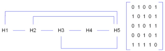
In this section, we present a method based on a GA to predict the graph whose vertices represent the SSE and edges represent spatial interactions between two amino acids involved in two different SSE, further this graph is called Secondary Structure Interaction Network (SS-IN),
Figure 7: 2OUF SS-IN (left) and its associated incidence matrix (right). The vertices represent the different α -helices and an edge exists when two amino acids interact.
see Fig 7.
6.2
Dataset
Thereafter, we use a dataset composed of proteins which have not fold families in the SCOP v1.73 classification and for which we have associated a family in [11].
6.3
Overall description
The GA has to predict the adjacency matrix of an un-known sequence when it is represented by a chromosome. Then, the initial population is composed of proteins of the associated family with the same number of SSEs. During the genetic process, genetic operators are applied to create new individuals with new adjacency matrices. We want to predict the studied protein adjacency matrix when only its chromosome is known.
Here, we represent a protein by an array of alleles. Each allele represents a SSE notably considering its size that is the number of amino acids which compose it. The size is normalized contributing to produce genomes whose alleles describe a value between 0 and 100. Obviously, the position of an allele corresponds to the SSE position it represents in the sequence. In the same time, for each genome we associate its SS-IN incidence matrix.
The fitness function we use to evaluate the performance of a chromosome is theL1distance between this chromo-some and the target sequence.
6.4
Genetic operators
Our GA uses the common genetic operators and also a specific topological operator.
The crossover operator uses two parents to produce two children. It produces two new chromosomes and matri-ces. After generating two random cut positions, (one ap-plied on chromosomes and another on matrices), we swap respectivaly the both chromosome parts and the both ma-trices parts. This operator can produce incidence matri-ces which are not compatible with the structural family, the topological operator solve this problem.
1%) of the generated children. It modifies the chromo-some and the associated matrix. For the chromochromo-somes, we define two operators: the two position swapping and the one position mutation. Concerning the associated matrix, we define four operators: the row translation, the column translation, the two position swapping and the one position mutation.
These common operators may produce matrices which describe incoherent SS-IN compared to the associated se-quence fold family. To eliminate the wrong cases we de-velop a topological operator.
The topological operator is used to exclude the incom-patible children generated by our GA. The principle is the following; we have deduced a fold family for the se-quence from which we extract an initial population of chromosomes. Thus, we compute the diameter, the char-acteristic path length and the mean degree to evaluate the average topological properties of the family for the particular SSE number. Then, after the GA generates a new individual by crossover or mutation, we compare the associated SS-IN matrix with the properties of the initial population by admitting an error rate up to 20%. If the new individual is not compatible, it is rejected.
6.5
Algorithm
Starting from an initial population of chromosomes from the associated family, the population evolves according to the genetic operators. When the global population fitness cannot increase between two generations, the process is stopped, see Algorithm 2.
The genetic process is the following: after the initial pop-ulation is built, we extract a fraction of parents according to their fitness and we reproduce them to produce chil-dren. Then, we select the new generation by including the chromosomes which are not among the parents plus a fraction of parents plus a fraction of children. It remains to compute the new generation fitness.
Algorithm 2:Genetic algorithm for SS-IN adjacency matrix determination.
Data:
pop: Current chromosome population parents: Set of parents
children: Set of children
begin
pop ←−setInitialPopulation()
while fitness(pop) is increasing do parents←−parentExtraction(pop)
children←−parentCrossing(parents)
children←−childrenMutation(children)
children←−exclusionByTopology(children)
pop ←−selection(pop, children)
0 10 20 30
[1-5] [6-10] [11-15] [16-20] [21-[
Error Rate
Initial population All alpha dataset
0 10 20 30
[1-5] [6-10] [11-15] [16-20] [21-[
Error Rate
Initial population All beta dataset
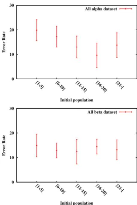
Figure 8: Error rate as a function of the initial population size. When the initial population size is more than 10, the error rate becomes less than 15%.
When the algorithm stops, the final population is com-posed of individuals close to the target protein in terms of SSE length distribution because of the choice of our fitness function. As a side effect, their associated matri-ces are supposed to be close to the adjacency matrix of the studied protein that we want to predict.
In order to test the performance of our GA, we pick ran-domly three chromosomes from the final population and we compare their associated matrices to the sequence SS-IN adjacency matrix. To evaluate the difference between two matrices, we use an error rate defined as the number of wrong elements divided by the size of the matrix. The dataset we use is composed of 698 proteins belonging to theAll alphaclass and 413 proteins belonging to theAll betaclass. A structural family has been associated to this dataset in [11].
Figure 9: SSE-IN of 1DTP protein. The edges we want to predict are green.
7
Conclusions
In this paper, we present two models to study the protein folding problem. The first try to reproduce the boid be-haviors when a protein is represented by the HP model. It implies that the hydrophobic amino acids tend to group to reproduce the general folded protein shape that is the hydrophobic side chains are packed into the interior of the protein creating a hydrophobic core and a hydrophilic surface. Second, we summarize relative works about how to fold an amino acid interaction networks. We need to limit the topological space so that the folding predictions become more accurate. We propose a genetic algorithm trying to construct the interaction network of SSEs (SS-IN). The GA starts with a population of real proteins from the predicted family. To complete the standard crossover and mutation operators, we introduce a topo-logical operator which excludes the individuals incompat-ible with the fold family. The GA produces SS-IN with maximum error rate about 25% in the general case. The performance depends on the number of available sample proteins from the predicted family, when this number is greater than 10, the error rate is below 15%.
The characterization we propose constitutes a new ap-proach to the protein folding problem. Here we propose to fold a protein SSE-IN relying on topological properties. We use these properties to guide a folding simulation in the topological pathway from unfolded to folded state.
7.1
Future Research Direction
After we have predicted the motifs in SSE-INs, we con-tinue our folding process by predicting the interaction involved between amino acid in the folded protein, see Fig. 9.
To do that, we build a probability of node interaction between different SSEs and we use a comparative model to predict the quantity of inter-SSE edges to add. The probability that two amino acids interact as a function of
their physico-chemical properties is computed from the comparative model exploited during the family associa-tion. Finally, we use an ant colony system to predict the nodes involved when two SSEs are in contact. When two SSEs are in interaction, we predict the inter-SSE edges by an ant colony approach and we repeat the same process at the global level. By measuring the resulting SSE-IN, we remark that their topology depends on the local re-search. If, during the local folding, we collect the right edges (more than 75%) then the global score stays close to 76% of the real inter-SSE edges. These approaches and results are exposed in [10].
The researches leaded are now oriented around the global amino acid interaction network, 3DSE-IN. We describe these type of graphs and study their topological behavior [12]. We deduce that the loops fold locally with their neighbors and propose three steps to fold a protein when it is represented by amino acid interaction networks.
References
[1] Anfinsen, C.B., “Principles that govern the folding of protein chains,” Science, V181, N1, pp. 223-230, 1973
[2] Asai, K., Hayamizu, S., Handa, K., “Prediction of protein secondary structure by the hidden markov model,” Bioinformatics, V9, N2, pp. 141-146, 1992
[3] Atilgan, A.R., Akan, P., Baysal, C., “Small-world communication of residues and signicance for protein dynamics,” Biophys J., V86, N(1 Pt 1), pp. 85-91, 2004
[4] Bairoch, A., Apweiler, R., “The swiss-prot protein sequence database and its supplement trembl,” Nu-cleic Acids Res, V28, N1, pp. 45-48, 2000
[5] Berman, H.M., Westbrook, J., Feng, Z., Gilliland, G., Bhat, T.N., Weissig, H., Bourne, P.E., Shindyalov, I.N., “The protein data bank,” Nucleic Acids Research, V28, N1, pp. 235-242, 2000
[6] Branden, C., Tooze, J.,Introduction to protein struc-ture, Garland Publishing, 1999.
[7] Dill, K.A, Bromberg, S., Yue, K.Z., Fiebig, K.M.,Yee, D.P., Thomas, P.D., Chan, H.S., “Prin-ciples of protein folding: A perspective from simple exact models,” Protein Science, V4, N4, pp. 561-602, 1995
[8] Dill, K.A., Chan, H.S., “From levinthal to pathways to funnels,” Nat. Struct. Biol., V4, N1, pp. 10-19, 1997
[10] Gaci, O., Balev, S., “Reconstructing Amino Acid Interaction Networks by an Ant Colony Approach,” J. Comput. Intell. Bioinformatics, V2, N3, pp. 131-146, 2009
[11] Gaci, O., “Building a topological inference exploiting qualitative criteria,” Online Journal of Bioinformat-ics, minor acceptation, 2010
[12] Gaci, O., “Community structure permanence in amino acid interaction networks,” Open Access Bioinformatics, in submission, 2010
[13] Gaci, O., and Balev, S., “Motif prediction in amino acid interaction networks,” Lecture Notes in Engi-neering and Computer Science: Proceedings of The World Congress on Engineering and Computer Sci-ence 2009, WCECS 2009, 20-22 October, 2009, San Francisco, USA pp. 8-13
[14] Ghosh, A., Brinda, K.V., Vishveshwara, S., “Dy-namics of lysozyme structure network: probing the process of unfolding,” Biophys J., V92, N7, pp. 2523-2535, 2007
[15] Kataoka, M., Goto, Y., “X-ray solution scattering studies of protein folding,” Folding Des., V1, N1, pp. 107-114, 1996
[16] Levinthal, C., “Are there pathways for protein fold-ing?,” J. Chim. Phys., V65, N1, pp. 44-45, 1968
[17] Levitt, M., Chothia, C., “Structural patterns in globular proteins,” Nature, V261, N1, pp. 552-558, 1976
[18] Mirny, B., Shakhnovich, L., “Protein structure pre-diction by threading: Why it works and why it does not,” J. Mol. Biol., V283, N2, pp. 507-526, 1998
[19] Muppirala, U.K., Li, Z., “A simple approach for pro-tein structure discrimination based on the network pattern of conserved hydrophobic residues,” Protein Eng. Des. Sel., V19, N6, pp. 265-275, 2006
[20] Murzin, A.G., Brenner, S.E., Hubbard, T., Chothia, C., “SCOP: a structural classification of the protein database for the investigation of sequence and struc-tures,” J. Mol. Biol., V247, N1, pp. 536-540, 1995
[21] Orengo, C.A., Michie, A.D., Jones, S., Jones, D.T., Swindells, M.B., Thornton, J.M., “CATH - a hier-archic classification of protein domain structures,” Structure, V5, N1, pp. 1093-1108, 1997
[22] Plaxco, K.W., Dobson, C.M., “Time-relaxed bio-physical methods in the study of protein folding,” Curr. Opin. Struct. Biol., V6, N1, pp. 630-636, 1996
[23] Reynolds, C., “Flocks, herds and schools: A dis-tributed behavioral model,”14th annual conference on Computer graphics and interactive techniques,