Abstract
A new C1 element is proposed to model Euler-Bernoulli beams in one and two-dimensional problems. The proposed formulation assures C1 continuity requirement without the use of rotational degrees of freedom, used in traditional elements, through the use of an Overhauser interpolation scheme for bending displacements. The principle of virtual displacements is used to determine the equilibrium equations and boundary conditions for one and two-dimensional Euler-Bernoulli beams. The Overhauser interpolation is introduced and the new bending interpolation functions are defined. Finally, beam and frame problems are solved with the new formulation and the results are compared to the traditional Euler-Bernoulli element and exact solutions.
Keywords
Finite Element, interpolation, Overhauser, beam.
A C
1
Beam Element Based on Overhauser Interpolation
1 INTRODUCTION
In the classical Euler-Bernoulli beam theory the main assumption is that the cross sections remain plane and orthogonal to the beam axis after deformation. This makes the beam shear undeformable and the shear stresses remain indeterminate. This theory presents good results for isotropic homo-geneous thin beams.
In order to account for shear, the assumption of orthogonality to the beam axis was removed by the Timoshenko beam theory, but the cross sections remain plane. Then, the beam is made shear deformable, but the predicted shear strain and stress proved to be constant through the beam thickness. Which is in contradiction with the principle that shear stress is zero at the beam surface. Therefore, a shear correction factor was introduced to account the effect of this deficiency of the Timoshenko beam theory.
André Schwanz de Lima a Alfredo Rocha de Faria b
a Instituto Tecnológico de Aeronáutica,
Department of Mechanical Engineering, São José dos Campos – SP, Brasil [email protected]
b Instituto Tecnológico de Aeronáutica,
Department of Mechanical Engineering, São José dos Campos – SP, Brasil [email protected]
http://dx.doi.org/10.1590/1679-78253142
The applications of those two theories in Finite Element Method are already standardized, as in Reddy (1993).
Other beam theories were formulated to include shear effects. Among those theories is the Red-dy third-order theory where the application for beams was developed as a specific case of plates. This theory was used by Heyliger and Reddy (1988) to develop a beam finite element and study bending and vibrations of isotropic beams.
Reddy (1997) later defined locking-free elements based on the simplified third-order theory, hav-ing the Euler-Bernoulli and Timoshenko solution as special cases. Such elements can be used to obtain exact nodal displacements and forces (from the equilibrium equations of the element) in a frame structural analysis using one finite element per structural member. Which is not achieved with the traditional equal interpolation, reduced integration element because the elements exhibit shear locking for thick members unless two or more elements per structural member are used.
Polizotto (2015) presented shear deformable beams of increasing order where a Reddy beam without shear coincides with the Euler-Bernoulli beam, and a Reddy beam shear deformable of infi-nite order can be identified with the Timoshenko beam.
Nevertheless, in all presented theories and their derived elements, rotational degrees of freedom are present in order to guarantee C1 continuity at the expense of increasing the number of degrees of freedom (DOF) necessary to model beams and frames. The objective of this work is to eliminate the rotational degrees of freedom related to bending and yet still satisfy the C1 continuity require-ment necessary for the convergence of the finite elerequire-ment method applied to beams, reducing the computational burden involved in the solution. In order to achieve this goal an Overhauser interpo-lation scheme will be used to generate a cubic interpointerpo-lation functions.
The new formulation proposed in the present work is developed based on the Euler-Bernoulli assumptions, where the rotational degrees of freedom are related to the transverse displacements derivatives only.
Overhauser (1968) proposed an interpolation scheme for curves and surfaces where, for curves, a linear blending of implicit parabolas defines a cubic interpolation between each pair of adjacent points, as an exclusive function of the point’s positions. Applying this concept to finite elements method, the beam and frame elements formulated in the present work possess cubic interpolation functions to represent bending based only in nodal displacements. But as it will be explained fur-ther, the application of the Overhauser interpolation is not straight forward and some solutions were proposed in order to incorporate such interpolation in finite elements formulation.
ap-proximated with Overhauser spline interpolation functions over boundary nodes but the geometry was completely decoupled from the finite element polynomial shape functions.
In the sequence of this work, the finite element formulation based on the classical beam theory for the beams and frames will be constructed using the principle of virtual displacements (PVD). The Euler-Bernoulli beam and frame interpolation functions will be briefly introduced. Then, Over-hauser interpolation will be presented and the new bending interpolation functions using Overhau-ser scheme will be developed and applied to one and two-dimensional formulations. Typical beam and frame problems will be solved using the new elements and results will be compared to the ana-lytical solution, for the one dimensional problems, and to the classical Euler-Bernoulli beam solution obtained using an academic license of the commercial Finite Element Analysis (FEA) software ABAQUS from Dassault Systèmes.
2 THE EULER-BERNOULLI BEAM FORMULATION
The governing equations of a three-dimensional beam can be obtained applying the Principle of Virtual Displacements (PVD). Then, one-dimensional and two-dimensional equations can be gener-ated with the correct simplifications.
The displacement field for a three-dimensional beam is represented by:
) ( ) ( ) ( ) ( ) ( ) ( ) ( x y x w w x z x v v x z x y x u u x x y z
(1)The strain-displacement relations are:
x x x y xz x x yz x x x z xy zz yy x y x z x xx
y
w
dx
w
d
dz
u
d
dy
w
d
dz
v
d
z
v
dx
v
d
dy
u
d
dz
w
d
dy
v
d
z
y
u
dx
u
d
, , , , , , ,0
0
0
(2)In the Euler-Bernoulli (classical) beam theory, it is assumed that the plane cross sections per-pendicular to the axis of the beam remain plane and perper-pendicular to the beam axis after defor-mation. Therefore z = v,x, y = -w,x and as a result the terms of the virtual work related to shear
vanish. Then, the strain-displacement relations become:
Another assumption of this theory is that no normal stresses are present in the y and z direc-tions. Along with the non-deformation of the cross-section, we can verify that yy = zz = yz = 0.
The principle of virtual displacement states: 0
i e
W W
(4)Where δWi is the virtual work of the internal strains and δWe is the external efforts virtual work.
The first term is defined as:
V T
i e dV
W { } {}
(5)
Where { } is a column matrix in the Voigt notation of the Cauchy tensor components and {δe} is a column matrix in the Voigt notation of the tensor [δe], this tensor is a quadratic function of the displacement gradients in Lagrangian coordinates.
Assuming the displacement gradients are small in modulus, compared to the unity, it is valid to approximate the displacement gradient with the components of the Green Strain Tensor. Then, the virtual work of the internal stresses can be written as
V T
i dV
W {
} {
}
(6)Applying the assumptions of the classical beam theory for an isotropic material δWi reduces to:
l x x y xx xx z xx xx xx xx
i EAu u EI w w EIv v GJ dx
W
0
, , ,
, ,
, ,
, )
(
(7)The virtual work of external loads for a three dimensional case considering distributed loads, concentrated forces and moments is written as:
0
, , , ,
(0) (0) (0) ( ) ( )
( ) (0) ( ) (0) (0) ( ) ( )
L
e x y z x y z x y
z x x x x y x z x y x z x
W q u q v q w dx Q u Q v Q w Q u L Q v L
Q w L T T L M w M v M w L M v L
(8)
As the main objective is to propose a formulation without rotational degrees of freedom for bending we can conclude that this formulation does not support, at first, prescribed moments as boundary conditions. But later, we will see that this is not entirely true. Also, three-dimensional applications, where torsion is involved, are impractical. Because in three-dimensional problems bending couples with torsion at the junctions of structural members with different orientations. Therefore, we cannot eliminate the degrees of freedom only related to bending. Reducing the ap-plicability of a three-dimensional element to structures composed by only one member. Then, no advantage arises from the use of the proposed element compared to the traditional Euler-Bernoulli element in 3D problems.
3 THE OVERHAUSER INTERPOLATION
Overhauser (1968) proposed that for a set of points, implicit parabolas are defined using three con-secutive points in a way that each adjacent pair of points belongs to two different parabolas. Then a linear blend of the two parabolas results in a C1 continuous cubic function.
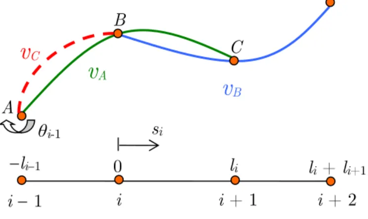
In order to apply this idea in finite element formulation, the points coordinates are replaced by the nodal transverse displacements and the implicit parabolas are converted into parabolic Lagrange interpolations of those displacements, as illustrated in Figure 1.
Figure 1: Overhauser interpolation scheme.
The si independent variable originally related to the arc-length is naturally linked to the length
of the elements. And the two parabolas vA and vB are defined as: 2 2 1 0 2
2 1
0
,
(
)
)
(
i i i B i i iA
s
a
a
s
a
s
v
s
b
b
s
b
s
v
(9)Where coefficients a0, a1, a2, b0, b1, b2 are functions of the nodal displacements vi-1, vi, vi+1 and vi+2.
The linear blending functions A and B are defined by:
i i A B
i i A
l
s
l
s
1
,
1
(10)defined in the interval 0 ≤ si ≤li.
Finally, the Overhauser curve, defined in the same interval is:
)
(
)
(
)
(
)
(
)
(
s
i As
iv
As
i Bs
iv
Bs
iv
(11)Evaluating the properties of such curve we notice that, as A and B are linear functions of si
and vA and vB are quadratic functions of si thus, the interpolation v(si) in Eq. 11 is a cubic function
of si. And if we evaluate the values of v at point i, the independent variable assumes zero value and
vA(si = 0) = vB(si = 0) = v(si = 0) = vi. Also, at point i+1, si = li and vA(si = li) = vB(si = li) =
v(si = li) = vi+1.
v
(
s
i)
l
i1l
il
i+
l
i+1s
ii
1
i
i
+ 1
i
+ 2
0
v
A(
s
i)
v
B(
s
i)
v
i-1v
iv
i+1The first derivative of v(si) is given by.
i B B i A A i B B i A A
i
ds
d
v
ds
d
v
ds
dv
ds
dv
ds
dv
(12)Then the first derivatives of v with respect to si at nodes i and i+1 are
)
(
)
(
,
)
0
(
)
0
(
i ii B i i i i
i A i
i
l
s
ds
dv
l
s
ds
dv
s
ds
dv
s
ds
dv
(13)
Therefore, it is seen that dv/dsi varies continuously in between each pair of adjacent points. So,
the curve v(si), can adequately represent an inflection that should occur within an interval. It
should be apparent that the cubic function defined in the interval between nodes i and i+1 does not pass through points i1 and i+2, this is an important difference in comparison to simple fit by cu-bic polynomials. The manner of construction (as a blend of two parabolas) guarantees that spurious wiggles will not be introduced, as frequently happens when simple cubics are forced to pass through four points of a curve.
However for the extremities, Overhauser (1968) uses the parabolic interpolation and the cubic interpolation derived applies only in the elements that share two parabolas, what we will call cen-tral elements (CE).
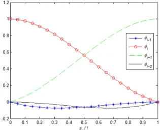
For those elements transverse displacement can be written as:
1 1 1 1 2 2
( )
i i i i i i i i iv s
v
v
v
v
(14)Where ϕi-1, ϕi, ϕi+1, and ϕi+2 are the interpolation functions for the central element (Eq. 28 in
Appendix A).
Those functions are defined in the interval 0≤ si ≤ li. Assuming all elements possess the same
length, li-1 = li = li+1 = l, we can plot the interpolation functions for a better understanding of its
behavior.
In Figure 2, we see clearly a local support character in the interpolation functions, and that the influence of the displacements of the nodes outside the element (i-1 and i+2) is much smaller than the ones of the element nodes (i and i+1).
Now, in order to construct cubic interpolation functions for the elements on the extremities, some considerations must be made. First, their interpolations must satisfy C1 continuity with the Overhauser interpolation already formulated for the central elements. Second, as it was said before, no rotational degrees of freedom are present, as a consequence, no essential nor natural boundary conditions of this character can be applied. Nevertheless, for many beam and frame problems this information is primordial.
Considering those points, a solution proposed is to build an element with a rotational degree of freedom only at the node not connected to central elements (first or last node of the structural member; i.e. node A in Figure 3). And then eliminate this degree of freedom via static condensation already considering the essential boundary condition. This strategy allows applying the different boundary conditions and accounting the effect of those boundary conditions in the element stiffness matrix.
Figure 3: New interpolation for left corner element.
For the left corner element, the new curve vC is a cubic defined in the interval li-1 ≤ si ≤ 0 by
the following equation.
3 3 2 2 1
0 i i i
C
c
c
s
c
s
c
s
v
(15)where coefficients c0, c1, c2 and c3 are obtained imposing the conditions,
1 1 1 2 1 3 1 2 1 0 3 1 3 2 1 2 1 1 0 1 1 ) 0 ( ) 0 ( ) ( 3 ) ( 2 ) ( ) 0 ( ) ( ) ( ) ( ) ( a s ds dv c s ds dv l c l c c l s ds dv c v s v l c l c l c c v l s v i i A i i C i i i i i i C i i C i i i i i i C (16)
A
B
C
l
i1l
il
i+
l
i+1s
ii
1
i
i
+ 1
i
+ 2
0
v
Av
Bv
Cwith a1 as the same coefficient from the parabola vA used in the blending of the central element to
obtain a cubic for the interval from i to i+1, and i-1 is the rotation in the point i-1.
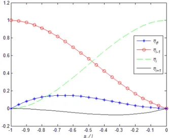
Then the curve vC can be written as a function of the nodal displacements and the rotation i-1
as:
1 1 1 1 1
C i i i i i i i
v
v
v
v
(17)Where θ, i-1, i, and i+1 are the interpolation functions for the left corner element (Eq. 29 in
Ap-pendix A). Again assuming all elements possess the same length, li-1 = li= li+1 = l, we can plot the
interpolation functions to understand its behavior.
Figure 4: Interpolation functions for the left corner elements assuming all elements possess the same length.
Again a local support character is observed in Figure 4, and we see that rotation influence is small, as also the displacement of the node outside the element (node C in Figure 3). But, as stated earlier, the main propose of this work is to eliminate the dependency of the rotational degrees of freedom. This can be accomplished by performing a static condensation of the degree of freedom i -1. The bending problem for the element can be written as:
1
11 12 13 14 1
1
21 22 23 24 2
31 32 33 34 3
1
41 42 43 44 4
[ ] { } { }
e eLCE LCE
e e e e e
i
e e e e e
i
e e e e e
i
e e e e e
LCE i LCE
K
v
f
K
K
K
K
f
v
K
K
K
K
f
v
K
K
K
K
f
v
K
K
K
K
f
(18)
Where [Ke]LCE is the stiffness matrix of the left corner element (LCE) and {f e}LCE is the respective
Considering the essential boundary condition of the node that possesses i-1, there are two
pos-sibilities that imply two different stiffness matrices and load vectors. If the node is clamped i-1 = 0,
then we just need to eliminate the first row and the first column of the matrix [Ke]LCE and the first
component of load vector {f e}LCE, resulting:
LCE e e e i i i LCE e e e e e e e e e
f
f
f
v
v
v
K
K
K
K
K
K
K
K
K
4 3 2 1 1 44 43 42 34 33 32 24 23 22 (19)But if this node is simply supported or free i-1 is unknown, then we have to isolate i-1 in the
first equation of the system presented in Eq. 18.
e i e i e i e e i
K
v
K
v
K
v
K
f
11 1 14 13 1 12 11
(
)
(20)Therefore, it is also possible to apply a concentrated moment at the degree of freedom i-1 when
we have this type of essential boundary condition. Then, the stiffness and load components related to i-1 are redistributed in an equivalent problem.
The elimination procedure in element level is only possible because the rotational degree of freedom is not shared with other elements. And as a result, the essential boundary condition is al-ready considered in the element level, being simply assembled in the global problem.
Figure 5: New interpolation for the right corner element.
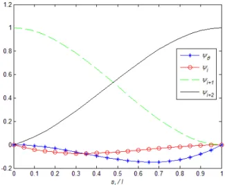
For the right corner element an analogous procedure is adopted to develop cubic curve vD and
the interpolation functions are defined in the interval 0 ≤x≤li+1 as presented in Figure 5, resulting:
2 2
2 1
1
i i i i i i iD
v
v
v
v
(21)The interpolation functions ψ , ψi, ψi+1, and ψi+2 presented in Eq. 30 of Appendix A and plotted
in Figure 6 (considering equal length for all elements) also guarantee C1 continuity with the central
E
F
G
l
il
i+1s
ii
1
i
i
+ 1
i
+ 2
0
v
A*v
B*v
D
l
i1
l
ielements and originate a stiffness matrix and load vector that consider the essential boundary con-dition at the unshared node.
Figure 6: Interpolation functions for the right corner elements assuming all elements possess the same length.
4 PLANE FRAME FORMULATION
For one-dimensional problems, the developed functions can be directly applied. But for two-dimensional analyses, some considerations must be made.
First, the axial displacements interpolation functions are the same linear interpolation functions used in traditional Euler-Bernoulli elements.
1
1
)
(
ii i i i i
i
u
l
s
u
l
s
s
u
(22)Consequently, as in traditional elements, only the degrees of freedom that belong to the element are taken in consideration. Contrary to the new bending formulation that uses information of nodes outside the element.
Second, the different orientations of the elements must be accounted and coherent transfor-mation matrices must be elaborated in order to correctly transform the stiffness and load compo-nents to the global coordinate system. As they were formulated the Overhauser interpolation func-tions for bending assume the same orientation for all nodes present in the cubic formulation.
Therefore, the transformation matrices must act also on the components related to the nodes external to the elements for the bending effects.
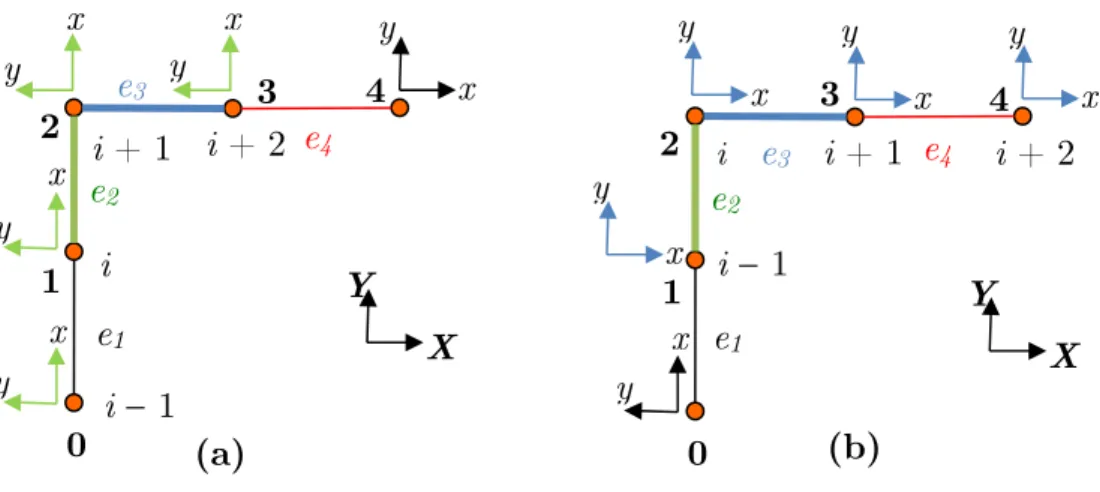
Figure 7: Nodes orientation for different elements.
Then, in element e2 (Figure 7.a), for node 3 a stiffness related to the transverse displacement y on the element (local) coordinate system would be transformed into a axial stiffness in the global coordi-nate system (GCS). This is not physically coherent nor numerically, inducing bad results. Because as stated before, axial behavior is not affected by nodes outside the element.
In the light of the above we propose that, when we have elements with different orientations sharing a node (i.e.: elements e2 an e3 sharing node 2 in Figure 7) we will treat each element that shares this node as left corner elements (LCE). With all matrices being generated including the rotational degree of freedom. Then, they will be transformed to the GCS and assembled in a super-element. Finally, the rotational degree of freedom can be eliminated by a static condensation proce-dure in element level analogous to the one presented before.
This solution numerically assures C1 continuity, avoids incoherent coupling of stiffness and al-lows representing structures such as the one presented in Figure 8, where elements e1, e3 and e5 share node 0. And e3 and e5 are rotated of α2 and α3 respectively, in relation to the GCS (element e1
LCS coincides with the GCS).
Figure 8: Example of elements with different orientations sharing the same node.
i
1
y
i
+ 1
i
+ 2
e
2x
y
x
y
x
i
x
y
2
0
1
3
4
X
Y
e
3e
4y
x
e
1(a)
i
1
i
+ 2
i
+ 1
e
2x
y
x
y
x
y
2
0
1
3
4
X
Y
e
3e
4x
y
x
y
e
1(b)
i
α
2e
2α
3e
1e
3e
5Y
X
0
1
2
3
4
e
4e
65
Once the stiffness matrices and load vectors of these three elements have been transformed to the GCS they can be assembled as presented in Figure 9.
Figure 9: Assembly of the stiffness matrices and load vectors of e1, e3 and e5.
Then, the elimination of the rotational degree of freedom 0 can be performed with a static con-densation, resulting the final stiffness matrices and load vector of the superelement, which can final-ly be assembled in the global stiffness matrix and load vector of the problem.
It is important to remark that the transformations to the global coordinates system should have been applied before the elimination and the assembly, if not, the stiffness related to the 0 will be
redistributed in a wrong way.
5 NUMERICAL RESULTS
Here we study the behavior of the Overhauser elements discussed on this paper. First, five one-dimensional analyses of different load conditions and essential boundary conditions are tested and compared to the exact solution according Euler-Bernoulli beam theory. Then, two frame problems are solved. For the convergence analysis, we adopted the criterion of 1% error in the displacements of specific points (not the whole structure) compared to the exact solutions for the beam problems, and compared to the Euler-Bernoulli solutions using ABAQUS for the frame problems.
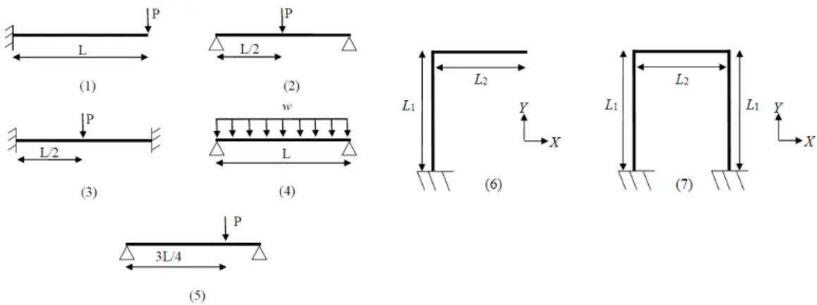
The beam and frame configurations tested are presented in Figure 10.
For all problems a linear elastic behavior was assumed and the following properties were adopt-ed: E = 210.0 GPa, = 0.3, L = L1= L2= 1 m. The cross section is circular (solid) of radius r = 0.0254 m and all elements possess equal length.
5.1 Beam Problems
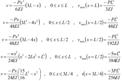
For the beam problems, the exact solutions using the classical beam theory according to Hibbler (2011) are:
EI PL L x v L x x L EI Px v 3 , 0 , 3 6 3 max 2 (23)
EI PL L x v L x x L EI Px v 48 2 / , 2 / 0 , 4 3 48 3 max 22
(24)
EI PL L x v L x x L EI Px v 192 2 / , 2 / 0 , 4 3 48 3 max 2 (25)
EI wL L x v L x L Lx x EI wx v 3845 2 / , 0 , 2 24 4 max 3 2 3 2 (26)
EI PL L x v L x x L EI Px v 2563 4 / 3 , 4 / 3 0 , 16 15 24 3 22
(27)
Where v is the transverse displacement, L is the beam length and x is the independent variable related to the length. And P represents the concentrated force, where in all cases a force P = 1000 N was applied, except for the distributed load case where a value of w = 1600 N/m was chosen in order to result the same maximum displacement of the force P. The maximum displacements were analyzed for the convergence tests, except for problem 5 where the displacement at x = 3L/4 was monitored.
Numerical Results
Problem 1 2 3 4 5
Elements to Convergence 9 18 40 16 20
vmax Exact (10-3 m) -4.8555 -0.3035 -0.0759 -0.3035 -0.1707*
vmax Overhauser (10-3 m) -4.8071 -0.3004 -0.0752 -0.3005 -0.1690*
Error (%) 0.9970 0.9970 0.9134 0.9794 0.9876*
* The values for problem 5 relates to the v(x = 3L/4).
Table 1: Numerical results of beam problems.
It is also noted that the essential boundary conditions influence the convergence rate. Compar-ing problems 2 and 3, where the natural boundary conditions are the same, but in 2 the extremities are simply supported and in 3 they are clamped, we see that the convergence rate reduces by half for problem 3, even with both solutions being cubic. This behavior is not observed with traditional Euler-Bernoulli elements for this situation. But if we compare problems 2, 4 and 5 with the same essential boundary conditions we see that the convergence rates are similar.
For problem 4, where not only the stiffness is integrated using the interpolation functions, but also the load, we see that results are coherent, indicating good behavior of the interpolation func-tions in this aspect.
Finally, post-processing was performed in order to extract information about nodal rotation v’(x) and maximum bending stress max(x) (at the nodes and element centroid) for all
one-dimensional problems.
C1 continuity was attested, confirming the mathematical formulation and also good behavior was attested concerning the critical points that were correctly captured. But as the displacement presented errors to the exact solution, those errors were passed to v’(x) and max(x) as consequence.
The errors to the exact solution as function of the beam length for v(x), v’(x) and max(x) are
presented in Figure 11 to Figure 13 respectively, on the domains where the exact solutions are de-fined (Eqs. 23 to 27).
Figure 11
Figure 13
In Figure 12 and Figure 13 the arrows indicate that the errors extrapolate. And for this reason, we preferred to indicate its tendency.
It is interesting to note that the essential boundary conditions interfere not only in the conver-gence rate but at the errors magnitude. As it was briefly explained before, the clamped and simply-supported/free elements have different stiffness matrices. Also, we see that for clamped situations, the errors are bigger at the corner elements decreasing in the other elements. While for the cases where simply-supported condition exists, the errors are bigger next to the points were v’ = 0 (criti-cal points). Where, for all problems in which a criti(criti-cal point occurs in central elements, the error in displacement tends to 1%, as presented in Figure 11.
The same tendency is observed in the nodal rotation errors presented in Figure 12. And in problem 5 the error in v’(x) next to the critical point rises until 23% closer to where the first deriva-tive changes sign. But as it was said before, the critical points are correctly captured.
Finally, concerning stresses, the corner elements are again the ones with the bigger errors, being the simply-supported / free corner elements the ones that exhibit the biggest errors, in the order of 73% for the problems 1, 2 and 5 where we have a concentrated force and 62% for problem 4 where we have a distributed load.
Therefore, we can conclude that both central and corner elements present errors, but it is clear that the proposed solution for the corner elements is more critical, especially when it comes to the second derivative of the interpolation functions.
5.2 Plane Frame Problems
For the frame problems the global coordinate system XY was defined in Figure 10 and the struc-tural members with length L1 are vertical (parallel to Y) and the ones with length L2 are horizontal (parallel to X).
The L-frame of problem 6 and the U-frame of problem number 7 both have clamped bases and elements with equal length were used.
such loading, only axial deformation of the vertical segments and simple translation of the horizon-tal segments should occur. What indeed happened, validating not only the solution, but the imple-mentation of the axial behavior as well, obtaining the same results of Euler-Bernoulli traditional elements within ABAQUS.
The same does not happen when we use central elements to model the edge. And a transverse deflection appears in both segments.
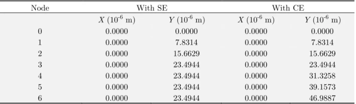
As an example, the displacements of L-frame structure with the force F1 = 104 N at the junc-tion of the structural members (see Figure 14) are presented in Table 2. The structure was modeled with six elements (three per structural member) using the superelement (SE) solution and also us-ing central elements (CE) at the junction.
Figure 14: L-frame with force F1 at the junction.
As stated before, modeling the junctions using central elements induces coupling between axial and transverse behavior that is not in accordance with the classical beam theory. This can be seen in the different nodal displacements on Y direction of the nodes of the horizontal member. But the superelement solution proved to be consistent with the problem physics.
Node With SE With CE
X (10-6 m) Y (10-6 m) X (10-6 m) Y (10-6 m)
0 0.0000 0.0000 0.0000 0.0000
1 0.0000 7.8314 0.0000 7.8314
2 0.0000 15.6629 0.0000 15.6629
3 0.0000 23.4944 0.0000 23.4944
4 0.0000 23.4944 0.0000 31.3258
5 0.0000 23.4944 0.0000 39.1573
6 0.0000 23.4944 0.0000 46.9887
Table 2: Nodal Displacements for L-frame with force F1 at the junction.
5 6
Y
X
F
11 2
3 4
0
L
1For the L-frame other two loading situations were tested, as shown in Figure 15.
Figure 15: Other load cases for L-frame.
The convergence criterion was 1% error in both X and Y displacements of the free end.
First a force F2 = 1000 N was applied. This problem resembles the cantilever beam problem analyzed before. Convergence was indeed achieved using the same nine elements in the vertical segment (18 elements for the whole structure, see Figure 17) as in the cantilever beam and no axial displacement was exhibited by the nodes in the vertical member, as the classical theory dictates. Also, the displacements in the nodes of the horizontal member (nodes 9 to 18 for the converged solution) in the X direction increase linearly, as shown in Figure 16. Also in accordance with the classical beam theory.
Figure 16: Nodal X-Displacements in the horizontal member.
Figure 17: Mesh convergence test for L-frame with load F2 at the free end.
Y
X L1
L2
F2
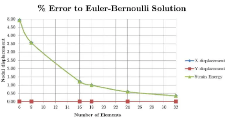
Second, the horizontal force F2 was replaced by a vertical force F3 = 100 N at the same point. Inducing bending in both members and axial deformation in the vertical member. The mesh con-vergence test in Figure 18 shows that the solution achieved the concon-vergence criterion with already eight elements (four per structural member). Also it reveals that the X-displacement of the end-node is the same that the one obtained using Euler-Bernoulli traditional elements even with six elements.
Figure 18: Mesh convergence test for L-frame with load F3 at the free end.
Comparing the two load cases and their respective convergence analyses (Figure 17 and Figure 18), we see that, curiously, the displacements in the direction of the concentrated force are the ones that present error. And strain energy percent error of the structure coincides with the percent error in the displacement in that direction. This indicates that bending is the dominant phenomena in terms of energy.
Also, the differences in the convergence rates indicate that, the solution is somehow sensible to the direction of the force and the presence of bending in one or more members.
Finally, the U-frame under multiple forces according to Figure 19 was analyzed, where F1 = -500 N and F2 = 1000 N are in the Y direction and F3 = 1000 N is in the X direction. In this case, all members are under bending and axial solicitations.
Figure 19: U-frame multiple load test.
L
1L2
F
2F
1Y
X
L
1The convergence criterion adopted was 1% error to the Euler-Bernoulli traditional element in both X and Y displacements of the junction where F2 and F3 were applied.
Solution converged using 60 Overhauser elements (20 per structural member), as illustrated in Figure 20, much more than both situations of the L-frame.
Figure 20: Mesh convergence test for U-frame with multiple loads.
Also, we can note that the error associated to the X-displacement is bigger, and this is the di-rection where bending displacements are more expressive, as it happened in the L-frame tests. Con-cerning the strain energy, again we attest that bending is the dominant phenomena, therefore the percent error in energy coincides the percent error in X-displacement (principal bending direction).
Finally, for all frame tests that involved bending, the same behavior of bigger errors in the nod-al transverse displacements closer to the clamped edges is exhibited, as it happened in the clamped beam problems. Revealing that despite the cubic interpolation functions, the Overhauser solution is less accurate, especially for the clamped corner elements.
6 CONCLUSIONS
In this paper, we formulated C1 beam finite element based on Overhauser interpolation and the Euler-Bernoulli beam theory that goes without the use of rotational degrees of freedom to represent bending.
Also we have seen that solution is much more influenced by the essential and natural boundary conditions compared to the traditional Euler-Bernoulli elements, especially the corner elements. It is not a trivial question to be answered why this influence of the boundary condition occurs and why the cubic interpolation does not represent the solution as well as the Hermite cubics. But the article brings this important breakthrough in understanding such interpolation as this is still a difficulty to be overcome by the proposed interpolation class. A future work suggestion is to investigate the use of different element sizes for the extremities, to evaluate the influence of such elements in the be-havior of the whole structure.
Finally, the application of such formulation is restricted to one and two-dimensional problems because torsion cannot be represented in the classical beam theory, without the use of a rotational degree of freedom, that in complex frame structures, couples with bending rotations.
References
Archer, R. (2006). Continuous solutions from the Green element method using Overhauser elements. Applied Numer-ical Mathematics 56:222-229.
Hadavinia, H., Travis, R.P., Fenner, R.T. (2000). C1-continuous generalised parabolic blending elements in the Boundary Element Method. Mathematical and Computer Modelling 31:17-34.
Hall, W.S. and Hibbs, T.T. (1987). The treatment of singularities and the application of Overhauser quadrilateral boundary element to three-dimensional elastostatics, In IVTAM Sympo. on Advance BEM, San Antonio, TX. Hall, W.S. and Hibbs, T.T. (1988). C1 continuous quadrilateral boundary elements applied to three dimensional problems in potential theory, In Boundary Element X (Edited by C.A. Brebbia) 1:181-192.
Heyliger P.R. and Reddy, J.N. (1988). A higher-order beam finite element for bending and vibration problems. Jour-nal of Sound and Vibration 126(2):309-326.
Hibbler, R. C. (2011). Mechanics of Materials, 8th edition, Pearson Prentice Hall, NJ.
Overhauser, A.W. (1968). Analytical definition of curves and surfaces by parabolic blending (Technical Report No: SL68-40), Ford Motor Company (Dearborn, Michigan).
Polizzotto, C. (2015). From the Euler–Bernoulli beam to the Timoshenko one through a sequence of Reddy-type shear deformable beam models of increasing order. European Journal of Mechanics - A/Solids 53:62-74.
Reddy, J.N. (1993). An Introduction to the Finite Element Method, 2nd edition, McGraw-Hill, New York.
Reddy, J.N. (1997). On locking-free shear deformable beam finite elements. Computer Methods in Applied Mechan-ics and Engineering 149: 113-132.
Taigbenu, A.E. (1998). Numerical stability characteristics of a Hermitian Green element model for the transport equation. Engrg. Anal. Boundary Elements 22:161–165.
Ulaga, S., Ulbin, M., Flašker , J. (1999). Contact problems of gears using Overhauser splines. International Journal of Mechanical Sciences 41:385-395.
APPENDIX A
Interpolation functions for the central elements:
1 1 1 1 2 2
2
2 3
1
1 1 1 1 1 1
2 2 2 2 2
1 1 1
1 1 1 1 1 1
( )
2 1
( ) 1 ( )
1
i i i i i i i i i
i i
i i i i
i i i i i i i i i i i i
i i i i i i i i i
i i
i i i i i i i i i i i i i
v s v v v v
l l
s s s
l l l l l l l l l l l l
l l l l l l l l l s
l l l l l l l l l l l l l
2 2 1 1 1 3 1 11 1 1 1
2 2 2
1 1 1 1
1
1 1 1 1 1 1 1 1
( ) 1
( ) 1
i i i i i
i i i
i i i i i i i i i i
i i i i i
i i
i i i i i i i i i i i i i i i i
s l l l l
l l l
s l l l l l l l l l
l l l l l
s
l l l l l l l l l l l l l l l l
2 3 1 11 1 1 1
2 3
2
1 1 1 1
( ) 1
1
i i
i i i
i i i i i i i i i i
i
i i i
i i i i i i i i
s l l l l
s l l l l l l l l l
l
s s
l l l l l l l l
(28)
Interpolation functions for the left corner elements:
1 1 1 1 1
2 3
2
1 1
2
1 2 1 3
1 2 3
1 1 1 1 1 1
( )
1 1
3 2
( ) ( ) ( )
C i i i i i i i i
i i
i i
i i i i i i
i
i i i i
i i i i i i i i i i i i
v s v v v
s s l l
l l l l l l l
s s s
l l l l l l l l l l l l
22 2 2 2
1
2 3
1 1 1
2 3
1 1 1 1 1 1
2
2
1 1
1
1 1 1 1 1 1
3 2 1 ( ) ( ) ( ) 2 1 ( ) ( ) ( ) i i
i i i i i i
i i i i
i i i i i i i i i i i i
i i
i i i
i i i i i i i i i i i i
l l l l l l l l
s s s
l l l l l l l l l l l l
l l
s s
l l l l l l l l l l l l
3 i s (29)
Interpolation functions for the right corner element:
1 1 2 2 2
2 3 2 1 1 2 2 3 1 1
1 1 1 1 1 1
2 2 2
1 1 1
1 1 1 ( ) 1 1 2 1 ( ) ( ) ( ) 2 3 1 ( )
D i i i i i i i i
i i
i i
i i
i i i i
i i i i i i i i i i i i
i i i i
i i
i i i i
v s v v v
s s
l l
l l
s s s
l l l l l l l l l l l l
l l l l
s l l l l
2 2 1 2 3 2 3
1 1 1 1
2
1 2 1 3
2 2 3
1 1 1 1 1 1
3 2
( )
i i i i
i i
i i i i i i i i
i i i i i i
i
i i i i
i i i i i i i i i i i i
l l l l
s s
l l l l l l l l
l l l l l l
l
s s s
l l l l l l l l l l l l