www.adv-radio-sci.net/9/309/2011/ doi:10.5194/ars-9-309-2011
© Author(s) 2011. CC Attribution 3.0 License.
Radio Science
A low-noise high dynamic-range time-domain EMI measurement
system for CISPR Band E
C. Hoffmann1and P. Russer2
1Technische Universität München, Lehrstuhl für Hochfrequenztechnik, Munich, Germany 2Technische Universität München, Lehrstuhl für Nanoelektronik, Munich, Germany
Abstract. In this paper, a broadband time-domain EMI measurement system for measurements from 9 kHz to 18 GHz is presented that allows for compliant EMI mea-surements in CISPR Band E. Combining ultra-fast analog-to-digital-conversion and real-time digital signal process-ing on a field-programmable-gate-array (FPGA) with ultra-broadband multi-stage down-conversion, scan times can be reduced by several orders of magnitude in comparison to a traditional heterodyne EMI-receiver. The ultra-low system noise floor of 6–8 dB and the real-time spectrogram allow for the characterisation of the time-behaviour of EMI near the noise floor. EMI measurements of electronic consumer devices and electric household appliances are presented.
1 Introduction
Electromagnetic interference (EMI) and electromagnetic compatibility (EMC) are traditionally measured on hetero-dyne EMI-receivers (Hagenhaus, 1942). The sequential mea-surement of typically several thousand frequencies yields long scan times on the order of hours or even days. Time-domain measurement systems can reduce scan times by sev-eral orders of magnitude. After broadband sampling of the EMI signal, the spectrum is calculated via the Fast-Fourier-Transform (FFT) and detectors are applied digitally. With the presented system, an EMI measurement over the complete band from 9 kHz to 18 GHz with an IF-bandwidth of 9 kHz takes less than 3 min. Using a traditional EMI-receiver with a dwell-time of 100 ms, the measurement of roughly 2×10⁶ frequency points would take over 55 h.
The standardization and development of new communi-cation technologies like WIMAX is attended by an
increas-Correspondence to:C. Hoffmann
ing usage of higher frequency bands in the high microwave range. This development implies the need for fast and com-prehensive EMI measurements in the frequency range above 1 GHz.
The presented time-domain EMI measurement system allows for the CISPR-compliant measurement of EMI in CISPR Band E up to 18 GHz. The real-time capability permits the characterisation of the time-behaviour of a de-vice’s emission. Spectrogram measurements of the data transmission between two modern smartphones and the non-stationary radiated emission of a microwave oven are shown.
2 Time-Domain EMI measurement system
The block diagram of the presented time-domain EMI mea-surement system is shown in Fig. 1. The EMI-signal is re-ceived by a broadband antenna for radiated emission or a line impedance stabilization network (LISN) for conducted emission. For measurements from 9 kHz to 1.1 GHz, the in-put signal is filtered by a lowpass filter to prevent spectral overlap due to a violation of Shannon’s theorem. The fil-tered signal is sampled by the floating-point analog-to-digital converter (Braun and Russer, 2005) with a sampling rate of around 2.6 Gs/s. An FPGA computes the signal spectrum via the FFT and weights the spectrum. The amplitude spectrum is displayed.
2.1 Fast-Fourier-Transform
To compute the EMI signal spectrum, the digitized EMI-signal is transformed by FFT. The FFT is an efficient algo-rithm for the computation of the Digital-Fourier-Transform (DFT). The FFT exploits symmetry and repetition properties and is defined as (Oppenheim and Schafer, 2009)
X[k] =
N−X1
n=0
LP
Floating Point ADC
Amplitude Spectrum
1.1 – 18 GHz 9 kHz – 1.1 GHz
Multi-Stage Broadband Down-Converter
Time-Domain Measurement System
LISN
FPGA FFT DDC Detectors
Fig. 1.Time-domain EMI measurement system.
8
8
t fD
2 cos
t
fD
2 sin
]
[t
x
]} [ Im{ut
]} [ Re{ut
Fig. 2.Digital down-conversion, taken from Braun et al. (2009).
whereX[k]is the discrete amplitude spectrum of the discrete time signalx[n].
2.2 Short-Time-Fast-Fourier-Transform
The Short-Time-Fast-Fourier-Transform (STFFT) is defined as an FFT over a limited time-interval. A Gaussian window functionw[n]is applied, corresponding to the IF-filter of a conventional measurement receiver. By application of the STFFT, a spectrogram is calculated. The spectrogram is a FFT taken over a time-interval of the sampled time-domain signal. It depends on the discrete time coordinateτ of the window and the discrete frequencyk. The STFFT is calcu-lated by (Oppenheim and Schafer, 2009)
X[τ,k] =
N−X1
n=0
x[n+τ]w[n]e−j2π knN . (2)
2.3 Digital Down-Conversion (DDC)
In order to avoid data overflow in the signal processor and to enable real-time processing of the signal, the frequency range from DC to 1.1 GHz is subdivided into eight subbands with a bandwidth of 162.5 MHz each. For the in-phase and quadra-ture channel, a polyphase decimation filter reduces the sam-pling frequency in order to fulfill the Nyquist criterion. Ev-ery subband is digitally down-converted to the baseband and the subbands are processed sequentially (Braun and Russer, 2005). The output sampling frequency is 325 MHz, while the bandwidth is 162.5 MHz. The block diagram is shown in Fig. 2.
BP 1 BP 2
PLL 1 PLL 2
IF 1 IF 2
LNA
Fig. 3.1.1–6 GHz down-converter.
3 Multi-stage broadband down-converter
To overcome the limitations imposed by available analog-to-digital converters, an ultra-broadband multi-stage down-converter is used to extend the frequency range up to 18 GHz. The upper frequency limit of the time-domain measurement system was increased to 3 GHz (Braun et al., 2009), 6 GHz (Braun et al., 2010) and 18 GHz (Hoffmann et al., 2010) by the addition of the multi-stage broadband down-converter. The EMI signal from 1.1–6 GHz is down-converted to the frequency range below 1.1 GHz by the 1.1–6 GHz down-converter. The down-converted signal is sampled and the spectrum is calculated. The frequency band from 6–18 GHz is in a first step down-converted to the input range of the 1.1–6 GHz converter. In a second step, it is down-converted to the range below 1.1 GHz and sampled.
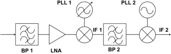
3.1 1.1–6 GHz down-converter
The block diagram of the 1.1–6 GHz down-converter is shown in Fig. 3. The EMI signal from 1.1–6 GHz is down-converted by two mixer stages. The input band is divided into 16 subbands with a bandwidth of 325 MHz each. The inher-ent overlap of the subbands is used to eliminate unwanted mixer spurious from the intermediate frequency band by a slight frequency shift of the subbands. The subbands are sequentially up-converted to a first intermediate frequency band IF 1 above the input band using a broadband mixer. The intermediate frequency band is filtered by the narrowband bandpass filter BP 2 and down-converted to the frequency range below 1.1 GHz by the second mixer. The local oscilla-tor frequencies are generated by low-noise PLL-synthesizers. Because of the nonlinear characteristics of the mixer, a large number of mixing products are generated at its out-put. These frequenciesfIF are determined by (Vendelin et al., 2005)
fIFm,±n= |m·fLO±n·fRF|, m,n∈N, (3)
wherefRF is the RF input frequency and fLO is the local
oscillator frequency.
If only the fundamental frequencies of fLO andfRF are
taken into consideration, i.e. m,n=1, we obtain two fre-quency components fRF 1,2 according to Eq. (3) (Maas,
Input-Band RF1
Mirror-band
RF2
IF1 LO-Band
Frequency f
Amp
li
tu
d
e
A
Band-Pass Filter
Fig. 4.Up-conversion frequency bands.
fRF 1,2= |fLO±fIF|. (4)
The frequency conversion yields two sidebands. The image-frequency signal is converted to the same intermediate fre-quency as the desired signal. Because the input band and the image band are not overlapping spectrally, the image band is sufficiently suppressed by the preselection bandpass filter BP 1 in this two-stage mixing scheme as illustrated in Fig. 4. The preselection band-pass filter also increases the spurious-free dynamic range of the system by suppressing low-frequency out-of-band EMI signal components. A high-gain, low-noise InGaP/GaAs MMIC preamplifier increases system sensitivity.
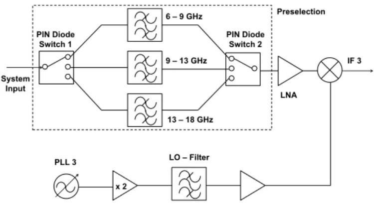
3.2 6–18 GHz down-converter
The block diagram of the 6–18 GHz down-converter is shown in Fig. 5. The input band is divided into 3 ultra-wide subbands: band 1 from 6–9 GHz, band 2 from 9–13 GHz and band 3 from 13–18 GHz. Broadband, low-insertion loss, single-input, triple-output (SP3T) PIN-diode switches are used to switch between the bands. Preselection filters increase system dynamic range. The EMI-signal is ampli-fied by a low-noise amplifier and down-converted to the fre-quency band from 1.1–6 GHz via a broadband mixer with low conversion loss. The local oscillator frequencies are gen-erated by a low-noise PLL-Synthesizer and an active multi-plier. Because the local oscillators fundamental is not suffi-ciently attenuated by the mixer’s LO-IF isolation, a fifth or-der planar bandpass filter is used to suppress the fundamental by over 75 dB.
3.3 Noise behaviour
With the signal-to-noise-ratios SNRin at the input and and
SNRoutat the output of a system, the system’s noise figureF
is given by (Davenport and Root, 1987)
F=SNRout
SNRin
. (5)
6 – 9 GHz
PLL 3
9 – 13 GHz
13 – 18 GHz
x 2
LO – Filter PIN Diode
Switch 1 PIN DiodeSwitch 2
IF 3 System
Input
LNA Preselection
Fig. 5.6–18 GHz GHz down-converter.
The available noise powerPNat the output of a system with
a noise figureF and unity gain is defined by
PN=kT0BENB, (6)
wherekis the Boltzmann constant,T0is the ambient temper-ature andBENBis the equivalent noise bandwidth. The noise power at the output of a system, that exhibits the noise figure
F can be calculated by
PN=F kT0BENB. (7)
For the calculation of the system noise figure above 1 GHz, the noise figures of the multi-stage broadband down-converter components up to the first mixer have been con-sidered. The noise figureF of a cascaded system with N
stages is determined by
F=1+F1+F2−1
G1
+F3−1
G1G2
+...+FN−1
N−Q1
k=1 Gk
, (8)
whereGi is the available power gain of stage i andFi is
the noise figure of stagei. With Eq. (8), the system’s noise figure was calculated to be less than 6 dB in the range from 1–6 GHz and less than 8 dB from 6–18 GHz.
The theoretical average system noise floor can be calcu-lated using Eq. (7). The equivalent noise bandwidthBENBof
the IF-filters with Gaussian characteristic is obtained with
BENB=
∞
Z
−∞
|H (f )|2df, (9)
using the filter’s transfer functions H (f ). This yields an equivalent noise bandwidth BENB,9 kHz of 6.8 kHz for the
Fig. 6.SP3T PIN-diode switch.
3.4 Dynamic range
EMI measurement systems have to exhibit a sufficient dy-namic range to be able to display transient emissions cor-rectly. The dynamic range of a system is limited by the sys-tem noise floor on the lower end and the maximum input level without distortion of the input signal on the upper end. For spectrum analyzers, the maximum level is typically the 1 dB compression point (P1dB) of the system. Heterodyne
EMI-receivers add a preselection to increase the dynamic range by suppressing out-of-band broadband or narrowband signals and Gaussian noise.
The preselection filter with the equivalent impulse band-widthBimp,preincreases the dynamic range for pulse signals
by
1Dpulse=20log10
Bimp,sys
Bimp,pre, (10)
with the equivalent impulse bandwidth of the measurement receiverBimp,sys.
For Gaussian noise, the dynamic range is increased by
1Dnoise=10log10
Bnoise,sys
Bnoise,pre, (11)
whereBnoise,sysandBnoise,pre are the equivalent noise
band-widths of the measurements receiver and preselection filter. Out-of-band narrowband signals with the frequency fn
are attenuated by the preselection filter’s transfer function
Hpre(f ). This yields an increase of dynamic range according
to
1Dn=20log10Hpre(fn). (12)
Pulse-modulated signals are used to determine the IF dynamic range of EMI measurement systems above 1 GHz. CISPR 16-1-1 (CISPR 16-1-1 Ed. 3.1 Am. 1, 2010) demands an IF dynamic range of at least 40 dB for EMI mea-surements above 1 GHz.
6 8 10 12 14 16 18
1 1.2 1.4 1.6 1.8 2 2.2 2.4 2.6 2.8 3
Frequency / GHz
Insertion Loss / dB
Insertion Loss Path 1 Insertion Loss Path 2 Insertion Loss Path 3
30 32 34 36 38 40 42 44 46 48 50
Isolation / dB
Isolation Path 2 (Path 1 ON) Isolation Path 3 (Path 1 ON)
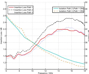
Fig. 7.Measurement of the SP3T PIN-diode switch.
4 Hardware implementation
As explained in Sect. 3.3, a low-noise figure of the first com-ponents in the RF Frontend is vital for maintaining a low system noise figure. PIN-diodes are commonly used in mi-crowave and millimeter wave switches and attenuators.
By variation of the stored chargeQ=IF·τ in the intrinsic
region of a PIN-diode, its series resistanceRScan be changed
by several orders of magnitude (Sze, 1988) according to
RS=
W2
IF·τ (µn+µp)
, (13)
whereWis the width of the intrinsic region,IFis the forward
bias current,τ is the minority carrier lifetime andµnandµp
are the electron and hole mobilities.
PIN-diode switches with single series diodes exhibit low insertion loss in the ON-state, but cannot provide the needed isolation in the OFF-state. To increase isolation, a series-shunt configuration was implemented, where dual series- shunt-diodes short-circuit the paths in the OFF-state in addition to the series diode in reverse polarity. The switches were fabricated on a glass reinforced hydrocarbon/ceramic RF-substrate and are shown in Fig. 6.
The performance characteristics of the switches were mea-sured with a vector network analyzer (VNA). The meamea-sured scattering parameters are shown in Fig. 7. The insertion loss for Path 1 and Path 3 is below 2.2 dB from 6–18 GHz. At 2.5 dB, the insertion loss of the middle path is around 0.3 dB higher, because of coupling to the other two paths. The iso-lation exceeds 30 dB at 18 GHz.
5 Measurement results
17.49810 17.499 17.500 17.501 17.502 20
30 40 50 60 70 80
Frequency / GHz
Magnitude / dBuV
Max Peak, 500 ms, IF 120 kHz, Att 20 dB Avg, 1 s, IF 120 kHz, Att 20 dB
Fig. 8.Measurement of a pulse-modulated signal.
a frequency of 17.5 GHz to the system input. The signal pulse width was set to 1 µs and the pulse period to 40 ms. The spectrum was weighted by peak and average detectors and is shown in Fig. 8. With this pulse period, the average detector already shows the system noise floor. The difference in level between the peak and average detector measurements is defined as the IF dynamic range. The measurements indi-cate an IF dynamic range of over 60 dB for an IF-bandwidth of 1 MHz, exceeding CISPR 16-1-1 requirements by over 20 dB.
Figure 9 shows the ultra-low system noise floor measured from 30 MHz to 6 GHz. The system exhibits a noise floor of below−15 dB µV in this range. To quantify the noise floor above 6 GHz, the noise voltagesVN were measured at
dis-tinct frequencies using the average detector and a matched input and the respective noise powersPN were calculated.
As the bandwidth of the used IF-filter with a Gaussian char-acteristic was 120 kHz, the resulting powers were normalized to an IF-bandwidth of 1 Hz, using
PNF,AV=PN/BENB,IF, (14)
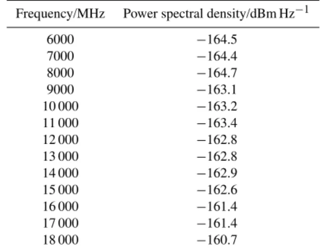
where PNF,AV is the average power of the system’s noise floor, andBENB,IFis the equivalent noise bandwidth of the IF-filter. The results are given in Table 1 and show that the system noise floor power spectral density from 6-18 GHz stays below−160 dBm Hz−1.
Measurements of the radiated emission of electronic con-sumer devices and electric household appliances were per-formed in a full anechoic chamber. A broadband quad-ridged horn antenna with a bandwidth from 1.7–20 GHz was used (Datasheet RF-Spin QRH20, 2010). To compensate for ca-ble losses and to give the electric field strength of the EMI, the corresponding transducer factors and the antenna factor were applied.
Figure 10 shows a spectrogram of the WI-FI data between two modern smartphones. The two phones formed a
wire-Fig. 9.System noise floor from 30 MHz to 6 GHz.
Table 1.System noise floor from 6 GHz to 18 GHz.
Frequency/MHz Power spectral density/dBm Hz−1
6000 −164.5
7000 −164.4
8000 −164.7
9000 −163.1
10 000 −163.2
11 000 −163.4
12 000 −162.8
13 000 −162.8
14 000 −162.9
15 000 −162.6
16 000 −161.4
17 000 −161.4
18 000 −160.7
less network and files were transmitted via the file-transfer-protocol (FTP). The antenna was placed in a distance of 3 m to the test subjects. The real-time spectrogram allows for the examination of the time-behaviour. While the WI-FI network was idle for the most part, the transmission of a file, lasting from 2 s to 6 s, is visible.
For the measurement shown in Fig. 11, a microwave oven was placed in a distance of 3 m to the antenna. The spectrum shows the magnetron’s fundamental at around 2.45 GHz and several higher harmonics up to 18 GHz. The scan time using an IF-filter bandwidth of 9 kHz and a frequency resolution of 50 kHz took around 120 s.
Frequency / MHz
Time / s
2440 2450 2460 2470 2480 2490 2500 2510
1
2
3
4
5
6
7
8
9
10
E−Field Strength / dBuV/m
10 20 30 40 50 60 70 80 90 100
Fig. 10.Spectrogram of WI-FI communication between two mobile phones.
2 4 6 8 10 12 14 16 18
20 30 40 50 60 70 80 90 100
Frequency / GHz
E
−
Field Strength / db
µ
V / m
Peak, 100 ms, IF 9 kHz, Att 10 dB AVG, 100 ms, IF 9 kHz, Att 10 dB
Fig. 11.Emission spectrum of a microwave oven.
of the magnetron’s 6th harmonic over a 20 s time-period. In a medium power setting, the magnetron turns on at around 2 s in time and turns off at 8 s. The change in frequency of the free-running oscillator is visible. The high sensitivity of the system and the real-time operation with an IF-bandwidth of 9 kHz enables the measurement of the 6th harmonic, which is located around 20 dB above the system noise floor.
6 Conclusions
A highly sensitive time-domain EMI measurement system for the frequency range from 9 kHz to 18 GHz was pre-sented. The system provides for EMI measurements in CISPR Band E in accordance to the requirements stated in
Frequency / GHz
Time / s
14.7 14.71 14.72 14.73 14.74 14.75 2
4
6
8
10
12
14
16
18
20
E
−
Field Strength / dBuV/m
45 50 55 60 65 70 75
Fig. 12.Spectrogram of the 6th harmonic of a microwave oven.
CISPR 16-1-1. In comparison to traditional EMI-receivers, scan times can be decreased by several orders of magni-tude. The high sensitivity, due to a low system noise floor of 6–8 dB, allows for the broadband characterisation of nar-rowband interference near the noise floor. Measurements of electric household appliances and consumer electronic de-vices were presented, including measurements of the sub-jects time-behaviour via the spectrogram.
Acknowledgements. The authors would like to thank the Bay-erische Forschungsstiftung and GAUSS Instruments GmbH, Mu-nich, Germany for funding this project and the EMV GmbH, Taufkirchen, Germany for supplying the antenna for the measure-ments. The authors are indebted to Stephan Braun and Arnd Frech from GAUSS Instruments GmbH for numerous helpful discussions.
References
Braun, S. and Russer, P.: A low-noise multiresolution high-dynamic ultra-broad-band time-domain EMI Measurement System, IEEE Transactions on Microwave Theory and Techniques, 53, 3354– 3363, 2005.
Braun, S., Hoffmann, C., and Russer, P.: A Realtime Time-domain EMI Measurement System for Measurements above 1 GHz, IEEE EMC Society Symposium on Electromagnetic Compati-bility, Austin, USA, 2009.
Braun, S., Hoffmann, C., and Russer, P.: Emissionsmessung im Zeitbereich oberhalb 1 GHz, EMV 2010, Düsseldorf, Germany, 2010.
CISPR 16-1-1, Ed. 3.1 Am. 1: Specification for radio disturbance and immunity measuring apparatus and methods Part 1-1: Ra-dio disturbance and immunity measuring apparatus – Measuring apparatus, International Electrotechnical Commission, 2010.
Datasheet RF Spin: Broadband Quad-Ridged Horn Antenna
QRH20, Data Sheet, 2010.
Hagenhaus, K.: Die Messung von Funkstörungen, Elektrotechnis-che Zeitschrift, 63, 182–187, 1942.
Hoffmann, C., Braun, S., and Russer, P.: A Broadband Time-Domain EMI Measurement System for Measurements up to 18 GHz, EMC Europe 2010, Wroclaw, Poland, 34–37, 2010. Maas, S. A.: Microwave Mixers, Artech House, 1993.
Oppenheim, A. V. and Schafer, R. W.: Discrete-Time Signal Pro-cessing, 3rd Edition, Pearson Prentice Hall, 2009.
Sze, S. M.: Modern Semiconductor Device Physics, John Wiley & Sons, 1988.