www.nat-hazards-earth-syst-sci.net/8/323/2008/ © Author(s) 2008. This work is distributed under the Creative Commons Attribution 3.0 License.
and Earth
System Sciences
Characterisation of the surface morphology of an alpine alluvial fan
using airborne LiDAR
M. Cavalli and L. Marchi
CNR-IRPI, Corso Stati Uniti 4 35127 Padova, Italy
Received: 14 September 2007 – Revised: 16 January 2008 – Accepted: 27 March 2008 – Published: 11 April 2008
Abstract. Alluvial fans of alpine torrents are both natural deposition areas for sediment discharged by floods and de-bris flows, and preferred sites for agriculture and settlements. Hazard assessment on alluvial fans depends on proper iden-tification of flow processes and their potential intensity. This study used LiDAR data to examine the morphology of the al-luvial fan of a small alpine stream (Moscardo Torrent, East-ern Italian Alps). A high-resolution DTM from LiDAR data was used to calculate a shaded relief map, plan curvature and an index of topographic roughness based on the standard de-viation of elevation within a moving window. The surface complexity of the alluvial fan, also influenced by human ac-tivities, clearly arose from the analysis. The surface rough-ness, defined here as the local topography variability, is com-pared with a previous classification of the fan surface based on field surveys. The results demonstrate that topographic analysis of ground based LiDAR DTM can be a useful tool to objectively investigate fan morphology and hence alluvial fan hazard assessment.
1 Introduction
Alluvial fans are gently sloping, fan-shaped landforms cre-ated by deposition of sediments often occurring at the base of mountain ranges. In Alpine valleys, alluvial fans have long been the preferred areas for agriculture and settlements. Therefore the deposition of sediment discharged by floods and debris flows, which causes alluvial fan formation and growth, represents a major hazard for human settlements. Debris flows are particularly dangerous because they pose a threat to the destruction of property and loss of lives in mountainous environments. The increasing human pressure
Correspondence to:M. Cavalli ([email protected])
on alluvial fans, which in the Alps is predominantly linked to tourism, requires accurate assessment of the hazard. In this context, the recognition of surface features on alluvial fans is essential for correct classification of torrent-related processes.
The identification of morphological features of alluvial fans, including the recognition of debris-flow deposits, old channels, levees and lobes, is commonly carried out by means of field surveys and interpretation of aerial pho-tographs. But these traditional methods are often problem-atic. Field surveys are time consuming and influenced by subjectivity, whereas the interpretation of aerial photographs is affected by uncertainty in forested areas. The airborne laser altimetry technology (LiDAR, Light Detection And Ranging) provides high-resolution topographical data, which can significantly improve the representation of land surfaces. A valuable characteristic of this technology is the capabil-ity to derive a high-resolution Digital Terrain Model (DTM) from the last pulse LiDAR data by filtering the vegetation points. In the field of geo-hydrological hazards in moun-tainous areas, the analysis of high-resolution DTMs is a promising approach to investigate fine-scale morphology of the landscape.
Fig. 1. Location map of the Moscardo Torrent basin and alluvial fan. The dashed line depicts alluvial fan boundary. Buildings are represented as black polygons. The line A–B indicates the section along which the profile of Fig. 2 was drawn.
Tarolli and Tarboton (2006) used LiDAR-derived DTMs to identify the optimal size of the cells for the assessment of shallow landslides. Staley et al. (2006) used LiDAR-derived topographic attributes (profile curvature and surface gradi-ent) for differentiating deposition zones on debris-flow fans. Frankel and Dolan (2007) combined quantitative measures of surface roughness, obtained from LiDAR data, with clas-sic methods of geomorphology and sedimentology to char-acterise and differentiate alluvial fan surfaces with different relative ages in an arid environment.
The purpose of this study is to test the capability of high-resolution LiDAR data to characterise the topography of an alpine alluvial fan. Particular attention was paid to discrimi-nating areas where debris-flow deposits are present from ar-eas in which these deposits are lacking. When compared to the study of alluvial fans with limited human influence under arid climate, the analysis of the topography of alluvial fans in the European Alps poses some additional problems. The hu-mid climate favours the growth of a dense vegetation cover, which reduces the density of measurements at the ground sur-face. Moreover, roads, buildings, torrent control works and other structures are often present on alluvial fans: this makes it necessary to distinguish the influence of natural features and man-made structures on the surface morphology of
allu-Fig. 2.Topographic profile of the alluvial fan drawn along the line A–B of figure 1.
vial fans.
In this study we use a LiDAR-derived DTM to analyse the surface morphology of an alluvial fan in the Italian Alps. The adopted approach encompasses the interpretation of shaded-relief and plan curvature maps and the comparison of a roughness index with a classification of the fan surface de-veloped on the basis of field surveys.
2 Study area
The study area is the alluvial fan of the Moscardo Torrent, a small stream of the Eastern Italian Alps (Fig. 1). Widespread erosion and instability phenomena in the upper basin slopes and along the main channel result in large amounts of loose debris being available for mobilization as debris flows during intense summer rainstorms; high channel slope produce an efficient delivery of the sediment to the basin outlet.
The Moscardo Torrent basin drains an area of about 4 km2 and ranges from 890 m at the fan apex to 2043 m at the high-est summit; the mean slope of the main channel is 20◦. The rocky substratum of the basin is made of Carboniferous fly-sch, represented by highly fractured and weathered shale, slate, siltstone, sandstone and breccia. Quaternary deposits, mostly consisting of scree and landslide accumulations, are common in the basin.
passes through the southern, no-longer active, portion of the fan (Fig. 1).
The climatic conditions of the Moscardo basin are typi-cal of the easternmost part of the Italian Alps, with abun-dant precipitation throughout the year, cold winters and mild summers. Average annual precipitation amounts to 1660 mm with 113 rainy days per year.
3 Methods
3.1 LiDAR data
The LiDAR data were acquired from an helicopter using an ALTM 3033 OPTECH, at an average altitude of 1000 m above ground level during snow-free conditions in Novem-ber 2003. The flying speed was 80 knots, the scan angle 20 degrees and the scan rate 33 KHz. The survey design point density was specified to be 2.5 points per m2, with first and last return recorded, and a vertical accuracy<15 cm. LiDAR point measurements were filtered into returns from vegeta-tion and bare ground using the TerrascanTMsoftware classi-fication routines and algorithms (Barilotti et al., 2006). The dataset covers most of the alluvial fan surface with the exclu-sion of a small area in the southern distal part. A 2 m grid size DTM from ground surface elevation points was generated by using Inverse Distance Weighted interpolation with a power of 2, a variable search radius with maximum distance of 3 m, and 3 as the number of nearest points to be used to perform the interpolation. The DTM grid spacing of 2 m was cho-sen as a compromise between the need for a fine-resolution DTM and the decrease of point density under canopy cover (about 0.25 points per m2)in the right side of the channel. The DTM from ground points was used to calculate a shaded relief map, a plan curvature map and an index of topographic roughness.
3.2 Shaded relief map
The shaded relief map was created with the Hillshade tool available in ArcGis 9.0 (ESRI, 2004), simulating illumina-tion from the northwest with an altitude angle of the illu-mination source of 45◦ above the surface. Hillshading en-hances the visualization of objects perpendicular to the az-imuth of the illumination; the planar and altitude angles of the illumination source were selected taking into account that important morphological features on the alluvial fan of the Moscardo Torrent, such as most old channels and gullies have prevailing E-W or NE-SW direction. Differently from more complex landforms (e.g. drainage basins with rugged relief), which would require different illumination points, a single view appears to be adequate for the alluvial fan under study.
3.3 Plan curvature map
The plan curvature map was created with LandSerf 2.2, a freely available software for digital terrain analysis (Wood, 1996; www.landserf.org). Plan curvature, which describes the rate of change of aspect, provides a measure of conver-gence and diverconver-gence of flow (Wilson and Gallant, 2000) and is often used for the identification of ridges and channels on digital terrain models (Rana, 2006; Haneberg et al., 2005). LandSerf 2.2, which calculates plan curvature on a cell-by-cell basis, utilises a quadratic function fitted to the surface using a moving window.
In this study we used an 11-cell moving window to de-rive the plan curvature map in order to smooth out features smaller than approximately 22 m wide. In the plan curvature map, a positive value indicates the surface is upwardly con-vex at that cell, whereas a negative value indicates the surface is upwardly concave at that cell, and a zero value corresponds to a flat surface.
3.4 Roughness index
The calculation of a roughness index is intended to measure the variability of elevations in local patches of the alluvial fan at a scale of a few meters.
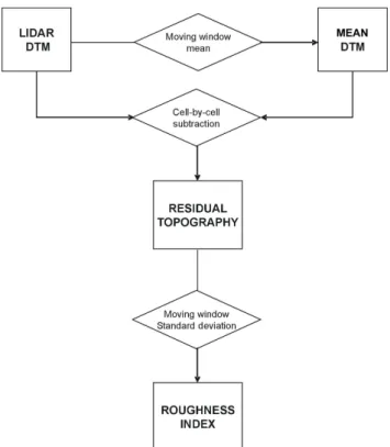
Several methods have been proposed to measure the sur-face roughness by LiDAR data (e.g. McKean and Roering, 2004; Haneberg et al., 2005; Glenn et al., 2006, Frankel and Dolan, 2007). In this work we define the surface roughness as the standard deviation of a residual topography (Cavalli et al., in press). A neighbourhood analysis was used to derive the roughness index of the Moscardo alluvial fan. Figure 3 shows the flow chart of the calculation of the roughness in-dex. A smoothed version of the LiDAR DTM (mean DTM in Fig. 3) was created by averaging elevation values within a 5-cell moving window. Each 5-cell of the mean DTM has a value corresponding to the mean of the 25 neighbourhood cells val-ues of the LiDAR DTM. The grid of residual topography was then calculated as the cell-by-cell difference between the Li-DAR DTM and the mean DTM. Finally, the standard devia-tions of residual topography values are computed in a 5-cell moving window over the residual topography grid. We de-fine the roughness index as:
σ = v u u u t 25 P
i=1
(xi−xm)2
25 (1)
whereσ is the roughness index or the standard deviation of residual topography, 25 is the number of the processing cells within the 5-cell moving window,xiis the value of one spe-cific cell of the residual topography within the moving win-dow, andxmis the mean of the 25 cells values.
Fig. 3.Flow chart of the roughness index calculation.
surface roughness by means of the residual topography grid provides a measure of this index independent from the effect of slope along the surface.
The benefit of the roughness index map analysis is in relat-ing values of surface roughness to different alluvial fan areas affected in the past by different flow processes: higher rough-ness values can be associated with debris-flow evidence on the alluvial fan surface and lower roughness values can be ascribable to smoother areas characterized by waterlaid de-position or artificially smoothed for agricultural expansion.
A map of the normalized distances from the fan apex was calculated in a similar manner to that of Staley et al. (2006), to analyse the spatial location and patterns of roughness in-dex values. The map of the normalized downfan distance calculated for each cell is given by the equation:
Dn= Da Dmax
(2) where Dn is the normalized downfan distance, Da is the planimetric distance of the cell from the fan apex, andDmax
is the maximum planimetric distance across the entire fan surface.
The planimetric distance map (Da) has been derived using the ArcGIS Distance tool, which allows calculation of the Euclidean distance of each cell from a source, represented in this case by the fan apex. To obtain the normalized downfan distance map (Dn) the values of each cell in the planimetric distance map has been then divided for the maximum value
of the map (Dmax)using the ArcGIS raster calculator (Eq. 2).
The values ofDnrange from 0, at the fan apex, to 1, at the farthest cell on the fan surface.
3.5 Field survey
The local topographic variability, represented by the rough-ness index, is compared with a previous classification of the fan surface, which was undertaken using field surveys com-plemented by interpretation of aerial photographs (Marchi and Cavalli, 2005). This field classification of the alluvial fan surface aimed to distinguish areas with evidence of de-bris flow from areas where sedimentary processes have lower solid concentration. Field observations led to identification of three classes:
– Class 1: areas where debris-flow deposits (lateral levees and terminal lobes) can be clearly recognized;
– Class 2: areas with remnants of past occurrence of de-bris flows (irregular fan surface and presence of large lone boulders);
– Class 3: no evidence of debris flow.
The absence of debris-flow deposits in Class 3 could in-dicate the dominance of bedload deposition (likely to have derived from the reworking of debris-flow deposits accumu-lated in the upstream parts of the alluvial fan). It is also possi-ble that deposits typical of debris flows have been obliterated by agricultural practices actively implemented on part of the alluvial fan until a few decades ago. This latter interpreta-tion hints at the low frequency of debris flows in these areas, as only areas rarely hit by debris flows were used for agri-culture. The classification of the alluvial fan surface into the three classes is presented in Fig. 4. We observe that the class with debris-flow evidences (Class 1) covers the active chan-nel and a limited area mostly located on its right side. Class 3 (no trace of debris flow) covers a wider area reaching the northern and southern boundaries of the alluvial fan, while the intermediate class (Class 2, with remnants of debris flow activity) has a limited extent and is situated between the other two classes.
3.6 Comparison of roughness index and field classification Statistical procedures were used to verify the consistency be-tween the values from the roughness index and the field clas-sification of the alluvial fan into three distinct classes. Both non-parametric and parametric tests were used for this com-parison.
Fig. 4.Terrain classification through field surveys: Class 1 indicates areas where debris-flow deposits (lateral levees and terminal lobes) can be clearly recognised; Class 2 are areas in which there is some evidence of a previous debris-flow occurrence; and Class 3 has no evidence of debris flows.
same population. This test compares one group to another group, therefore, in order to analyse the three classes, each class was compared to the other two.
The F-test is an overall test of the null hypothesis that group means on the dependent variable do not differ. A sig-nificant value ofF indicates that there are differences be-tween the means but does not indicate where these differ-ences are. Once a significant F-value was obtained in the analysis of variance, the Tukey’s Honestly Significant Differ-ence for unequal sample size post hoc test (Tukey HSD test) was performed to identify significant differences between in-dividual classes. This test compares the difference between each pair of means. These tests require normal distribution of the variables under study. In order to obtain normal distribu-tion of surface roughness data, a logarithmic transformadistribu-tion was applied.
The software Statistica for Windows (Statsoft, 2001) was used for this analysis.
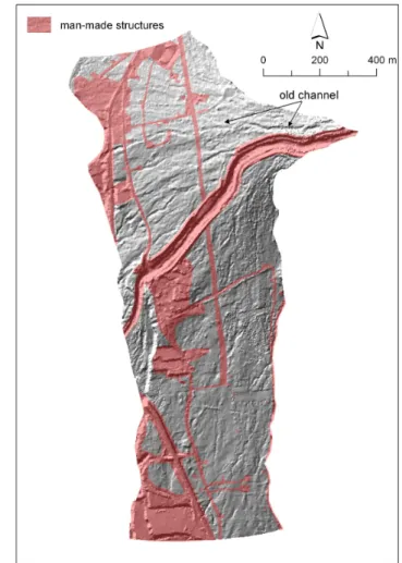
Fig. 5.Shaded relief map of the Moscardo Torrent alluvial fan. This representation enhances the visualization of objects perpendicular to the northwestern direction of the illumination. The man-made structures are outlined in red.
4 Results
The shaded relief map of the Moscardo alluvial fan is pre-sented in Fig. 5. The ability of laser shots to penetrate the vegetation canopy is highlighted in the shaded relief map, which reveals several subtle geomorphic features that are not visible in aerial photographs and in digital models of the ground surface derived from topographic maps. One such ex-ample is the track of an old channel of the Moscardo Torrent, partially covered by coniferous forest, located in the north-ern part of the fan that is obvious in Fig. 5. Even artificial structures (indicated by red areas in Fig. 5) are easily rec-ognizable. Buildings have been removed during the filtering process of LiDAR data but terrain embankments related to their presence are still identifiable.
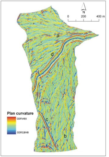
Fig. 6. Plan curvature map:(a)old channels, sometimes bordered by debris-flow levees,(b)flow directions of old channels and rills,
(c)national road,(d)Moscardo Torrent dikes.
with the flow directions of old channels and rills (prevailingly North to South) also outlined in the southern sector of the al-luvial fan (b in Fig. 6). Artificial structures shown clearly in the plan curvature map are the national road in the south-western sector of the alluvial fan and the dikes built along the Moscardo Torrent (c and d respectively in Fig. 6).
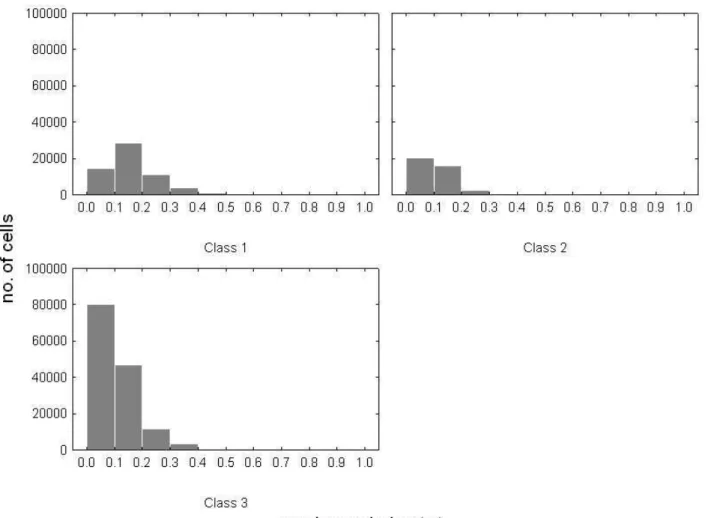
The roughness index map (Fig. 7) contributes to the recog-nition of morphological features by emphasizing local eleva-tion variability that may not be apparent on the shaded re-lief image. The surface roughness values for this alluvial fan ranged from 0 to approximately 1 m, although most of the values are <0.5 m (Fig. 8). Higher values of surface roughness can be found near the fan apex and along the main channel where debris-flow levees and lobes are present (a in Figs. 7 and 8). The distal areas of the fan are characterised by low values of roughness (c in Figs. 7 and 8), except where man-made structures, such as road embankments, increase local topographic variability.
As mentioned previously, the recognition of man-made structures is needed to avoid misinterpretation with natural
Fig. 7.Roughness index map:(a)area with high values of rugged-ness (debris-flow levees and lobes), (b) low values of roughness index along a pipeline,(c)distal areas of the fan with low values of the index,(d)high values of roughness emphasize the quarry de-posit,(e)isolated area with high values of roughness. See Figs. 8 and 12a for representative pictures. White continuous lines indicate the normalised downfan distance (cf. Fig. 10).
features. In Fig. 7a long strip with low values of roughness crossing the fan in the north-south direction can be recog-nized, which corresponds to a flat area alongside a pipeline (b in Figs. 7 and 8). More flat areas with low roughness val-ues are associated with the presence of buildings, which have been removed during the LiDAR data filtering process. An-other human-modified area corresponds to the quarry deposit to the left of the main channel and is characterized by high values of surface roughness (d in Fig. 7). An isolated, spa-tially limited area with relatively high roughness values can be distinguished in proximity of the eastern boundary of the fan (e in Fig. 7).
Table 1.Basic statistics for the surface roughness index (total study area).
Class no of DTM cells min max mean median std. dev. 1 60002 0.034 0.772 0.168 0.140 0.092 2 38918 0.023 0.540 0.112 0.098 0.056 3 143021 0.004 0.968 0.114 0.092 0.072
Table 2.Basic statistics for the surface roughness index (after the removal of man-modified areas).
Class no of DTM cells min max mean median std. dev. 1 45679 0.033 0.784 0.144 0.123 0.073 2 33934 0.024 0.489 0.107 0.097 0.046 3 86592 0.023 0.568 0.097 0.085 0.045
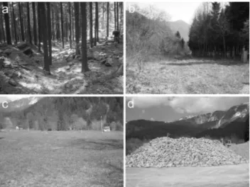
Fig. 8. Photographs of landforms related to the roughness index map (Fig. 7):(a)debris-flow deposits and levees,(b)a pipeline,(c)
distal fan area with a smoothed surface,(d)quarry deposit.
lower values are observed in the other classes, for both the whole fan area and also after the removal of man-modified areas (Tables 1 and 2). The artificially-lined channel of the Moscardo Torrent and its banks were included in man-modified areas (Fig. 5) because they are not representative of natural depositional processes on the alluvial fan.
As mentioned previously, both parametric (F-test and Tukey HSD test) and non-parametric statistical analyses (Mann-WhitneyUtest) were carried out to compare the val-ues of surface roughness in the three classes mapped from field surveys. The Mann-Whitney U test rejects the null hypothesis for all the comparisons (Class 1 vs. Class 2, p<0.001; Class 1 vs. Class 3,p<0.001; Class 2 vs. Class 3, p<0.001) both on the whole data set and after remov-ing human-altered areas. Therefore, the non-parametric test shows that individual classes are statistically different from
each other in term of surface roughness at the 99% con-fidence (α=0.01). The result of the F-test on the surface roughness values of the three Classes allows us to reject the null hypothesis (F=13773,p<0.001). The results indicate differences in the group means for each pair at the 99% con-fidence (α=0.01). These results are consistent with those obtained from the application of the non-parametric Mann-WhitneyUtest.
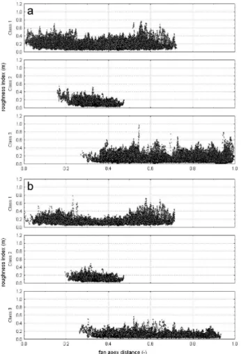
The scatterplot of the surface roughness versus the dis-tance from the fan apex for the three mapped classes makes it possible to analyze the pattern of roughness along the al-luvial fan. In Fig. 10a the entire data set is plotted: several peaks are present throughout the length in the scattergram both in Class 1 and Class 3. The peaks in Class 1 are located where debris-flow deposits and old levees are present, and also on the artificial banks of the main channel. The high-est values of roughness in Class 3 are found at a distance of 0.5–0.7 from the fan apex, which corresponds to the spatial location of the majority of artificial structures in the alluvial fan. Class 2 is characterized by a more regular pattern and the natural fan surface is accurately depicted due to the lack of human-modified areas.
In Fig. 10b the data without the man-altered areas are plot-ted. For ease of comparison, the values of the downfan distance in Fig. 10b were computed using the same value of Dmax as in Fig. 10a. Because of the removal of
Fig. 9.Histograms of roughness index values for the three classes mapped from field surveys.
5 Discussion
The results of the statistical tests indicate that the quanti-tative assessment of the surface roughness agrees with the visual interpretation of the morphology of the alluvial fan, from which the three classes of the fan surface were mapped, shown in Fig. 4. The consistency of the results of the non-parametric Mann-WhitneyUtest with the parametric analy-sis of log-transformed roughness data, confirms the stability of the results obtained. In this paper, the statistical analy-sis was aimed at comparing topographic roughness derived from a LiDAR DTM with a previous field classification of the fan surface. The use of spatial statistics for the auto-mated recognition of topographic features and classification of morphological units could represent an important step to-wards an enhanced use of data derived from aerial LiDAR in alluvial fan studies.
In addition to the quantitative analysis performed on roughness index values, the visual inspection of the maps of LiDAR-derived indicators can also contribute to the in-terpretation of the morphological features of the fan surface. In the previous section, the correspondence between values
of the roughness index and features observed in the field has been reported. Here we extend the discussion on this topic by comparing the capabilities of plan curvature and rough-ness index, and showing the potential of the roughrough-ness index in identifying areas with particular topographic features on the fan surface.
A valuable characteristic of plan curvature is that through the enhancing of concavities and convexities it is possible to identify linear features even in areas of low roughness, as is shown in the distal part of the alluvial fan in the Figs. 6 and 7. In contrast, linear features not marked by convex-ities and concavconvex-ities, such as the pipeline that crosses the alluvial fan of the Moscardo Torrent, are not clearly recog-nised in the plan curvature map. As previously reported, the flat strip alongside the pipeline is easily identifiable on the roughness index map (b in Fig. 7). A combined use of differ-ent indicators is thus advised for a reliable iddiffer-entification of natural and man-altered features.
Fig. 10.Scatterplot of roughness values versus normalized distance from the fan apex:(a)whole data set,(b)after removing man-made structures.
in Fig. 7, was not recognised by the field surveys and aerial photograph interpretation, which led to the classification of the alluvial fan proposed in Fig. 4. An East – West topo-graphic profile surveyed in the middle part of this area using a theodolite shows a close agreement with the LiDAR-derived DTM (Fig. 11), thus confirming that LiDAR elevation data represents the actual topography and are not affected by arti-facts induced by data filtering. The visual inspection of this area confirms the presence of a rugged surface with scattered large boulders (Fig. 12a), which contrasts with the smooth surface of neighbouring areas (Fig. 12b). The widespread presence of large boulders, which makes agricultural activity difficult, may have caused this area to undergo lesser topo-graphic alterations than other parts of the fan.
The Moscardo Torrent fan is characterized, like many al-luvial fans in alpine valleys, by the presence of forest cover and artificial structures. Forest cover poses major problems in the recognition of the features of alluvial fan surface by means of aerial photo interpretation. LiDAR data can help overcoming these problems, provided that adequate attention
Fig. 11. Topographic profile along the area indicated as “e” in Fig. 7.
Fig. 12. Photographs taken in: (a)the rugged-surface area (e in Fig. 7), and(b)in a neighbouring smooth area.
is paid in the creation of the DTM and deriving geomorphic attributes. Since the spatial variability of DTM roughness is strongly influenced by LiDAR points density, care has to be taken where the different land use leads to different spatial density of ground LiDAR points. In correspondence to dense vegetation cover, as with coniferous forest on the right side of the channel in the Moscardo alluvial fans, the density of ground points recorded in LiDAR surveys is markedly lower than in open areas (2.5 and 0.25 points per m2respectively). To correctly select the DTM grid spacing in an area with dif-ferent land uses, the spatial density of LiDAR points in the sector with the densest vegetation has to be taken into ac-count. In the present study, a grid spacing smaller than 2 m could have given rise to misinterpretation of topography un-der forest cover with respect to open areas. When planning aerial LiDAR surveys, a high sampling point is then recom-mended, as it can provide higher density even under forest canopy, thus allowing a smaller grid spacing of the DTM.
In Fig. 10b, which presents the relationship between sur-face roughness (ascribed only to natural features) and the dis-tance from the fan apex, no decrease of the roughness for increasing distance can be observed within each class. In particular, Class 1, which represents the most recent sedi-mentary processes, shows high values of the roughness in-dex in its distal part. This can be related to the efficient de-livery of debris-flows to the lower part of the alluvial fan of the Moscardo Torrent. The deposition of debris flows close to the active channel results in a rugged fan surface even at long distances from the fan apex.
Staley et al. (2006) used morphometric indexes from a LiDAR-derived DTM to identify three zones with different depositional features in 19 debris-flow fans in the Death Val-ley. They observed high values of profile curvature at the proximal locations of the fan surface and correlated them to deposits with high internal shear strength. Moderate values of profile curvature correspond to deposits with lower shear strength, whereas the lowest values of profile curvature oc-curred in run-out zones in the mid-fan section. Both the pro-file curvature used by Staley et al. (2006) and the roughness index proposed in this study are indicators of topographic variability correlated to the typology of alluvial fan deposits. Staley and colleagues state that their findings are not applica-ble at the scale of individual fans. However, it is interesting to note (Fig. 10b) that, similar to the profile curvature in the debris-flow fans studied by Staley et al. (2006), the rough-ness index in Class 1 of the Moscardo alluvial fan shows the lowest values in the intermediate part of the profile (i.e. the run-out area). This pattern is not recognisable in Classes 2 and 3, which are influenced by fluvial reworking of debris-flow deposits, bedload deposition and artificial smoothing of the surface for agricultural exploitation.
6 Conclusions
This paper has shown the potential of LiDAR-derived topo-graphic indexes in the analysis of the topotopo-graphic variations within an alpine alluvial fan, where both natural landforms due to debris-flow deposition and man-made structures are present. Different tools (shaded relief and plan curvature, roughness index) were used in the detection of topographic features of alluvial fan surface.
The statistical comparison of the values of the topographic index was contrasted with a previous visual classification of the alluvial fan according to the presence of debris-flow de-posits, and it was shown that there was consistency between the two approaches.
Man-made structures are often present on the alluvial fans of the European Alps and have a major influence on their surface topography. The analysis presented in this paper has shown that the presence of artificial structures on the allu-vial fan of the Moscardo Torrent, although not preventing the quantitative description of natural morphology, had a
non-negligible impact on the values of the roughness index (Ta-bles 1 and 2, and Fig. 10). Careful identification of artificial structures is thus recommended to avoid misinterpretation of LiDAR-derived topographic indexes. Digital photographs, commonly taken during aerial LiDAR surveys, are a good ba-sis for the identification of human-related entities, although field checks are also recommended for further verification.
The analysis presented in this paper would not have been possible using digital models of the ground surface derived from traditional topographic maps, not only because of the lower resolution obtainable, but, and probably more impor-tantly, also because of the lack of detail on local topography, especially under forest cover. Digital photogrammetry ap-plied to large-scale aerial photographs makes it possible to obtain high-resolution DTMs (Lin and Oguchi, 2004), but detailed recognition of fine topographic features is possible with this method only in unvegetated areas or those with sparse vegetation.
The GIS tools presented in this paper can contribute to the characterization, both qualitative and quantitative, of the surface morphology of alpine alluvial fans and are suitable for a combined use with traditional techniques, such as field surveys and aerial photo interpretation.
Acknowledgements. The LiDAR data used in this study are available thanks to the University of Udine (European Project INTERREG IIIA Phare CBC Italy-Slovenia, Action 3.2.4). We are grateful to M. Derron and M. Jaboyedoff for their valuable comments on the manuscript, and to L. Clarke for revising the English text.
Edited by: T. Glade
Reviewed by: M.-H. Derron and M. Jaboyedoff
References
Ardizzone, F., Cardinali, M., Galli, M., Guzzetti, F., and Reichen-bach, P.: Identification and mapping of recent rainfall-induced landslides using elevation data collected by airborne Lidar, Nat. Hazards Earth Syst. Sci., 7(6), 637–650, 2007.
Barilotti, A., Beinat, A., Fico, B., and Sossai, E.: Produzione e ver-ifica di DTM da rilievi LiDAR aerei su aree montane ricoperte da foresta, in: Convegno Nazionale SIFET 2006 Le nuove fron-tiere della rappresentazione 3D, Castellaneta Marina, Italy, 14– 16 June 2006, on DVD (in Italian), 2006.
Carter, W., Shrestha, R., Tuell, G., Bloomquist, D., and Sartori, M.: Airborne laser swath mapping shines new light on Earth’s topography, EOS, Transactions, American Geophysical Union, 82(46), 549–555, 2001.
Cavalli, M., Tarolli, P., Marchi, L., and Dalla Fontana, G.: The ef-fectiveness of airborne LiDAR data in the recognition of channel-bed morphology, Catena, available online, 26 December 2007, doi:10.1016/j.catena.2007.11.001, in press, 2008.
ESRI: ArcGIS 9.0 User’s Guide, Redlands, CA, 2004.
topographic data, J. Geophys. Res. – Earth Surface, 112, F02025, doi:10.1029/2006JF000644, 2007.
Glenn, N. F., Streutker, D. R., Chadwick, D. J., Thackray, G. D., and Dorsch, S. J.: Analysis of LiDAR-derived topographic informa-tion for characterizing and differentiating landslide morphology and activity, Geomorphology, 73, 131–148, 2006.
Haneberg, W. C., Creighton, A. L., Medley, E. W., and Jonas, D.: Use of LiDAR to assess slope hazards at the Lihir gold mine, Papua New Guinea, in: Proceedings, International Conference on Landslide Risk Management, Vancouver, British Columbia, May–June 2005, Supplementary CD, 2005.
Haugerud, R., Harding, D., Johnson, S., Harless, J., and Weaver, C.: High-resolution Lidar topography of the Puget Lowland, Wash-ington – A Bonanza for Earth Science, GSA Today, 4–10, 2003. Lin, Z. and Oguchi, T.: Drainage density, slope angle, and rela-tive basin position in Japanese bare lands from high-resolution DEMs, Geomorphology, 63, 159–173, 2004.
Marchi, L. and Cavalli, M.: Riconoscimento dei processi torrentizi in area di conoide e scenari di intensit`a, in: La prevenzione del rischio idrogeologico nei piccoli bacini montani della regione: esperienze e conoscenze acquisite con il progetto CATCHRISK, Regione Autonoma Friuli Venezia Giulia, Direzione centrale risorse agricole, naturali, forestali e montagna, Servizio territorio montano e manutenzioni, 113–143 (in Italian), 2005.
McKean, J. and Roering, J.: Objective landslide detection and sur-face morphology mapping using high-resolution airborne laser altimetry, Geomorphology, 57, 331–351, 2004.
Rana, S.: Use of Plan Curvature Variations for the Identification of Ridges and Channels on DEM, in: Progress in Spatial Data Han-dling, edited by: A. Riedl, W. Kainz, and G. Elmes, Springer-Verlag, Heidelberg, Germany, 789–804, 2006.
Schulz, W. H.: Landslides mapped using LIDAR imagery, US Ge-ological Survey, Seattle, Washington, Open File Report 2004– 1396, 11 pp., 2004.
Staley, D. M., Wasklewicz, T. A., and Blaszczynski, J. S.: Surfi-cial patterns of debris flow deposition on alluvial fans in Death Valley, CA using airborne laser swath mapping, Geomorphology, 74, 152–163, 2006.
Statsoft: STATISTICA System Reference, Statsoft, Inc., 2300 East 14th Street, Tulsa, Oklahoma, USA, 1098 pp., 2001.
Tarolli, P. and Tarboton, D. G.: A new method for determination of most likely landslide initiation points and the evaluation of digital terrain model scale in terrain stability mapping, Hydrol. Earth Syst. Sci., 10, 663–677, 2006,
http://www.hydrol-earth-syst-sci.net/10/663/2006/.
Wilson J. P. and Gallant J. C.: Digital Terrain Analysis, in: Terrain Analysis: Principles And Applications, edited by: J. P. Wilson and J. C. Gallant, John Wiley & Sons, New York, USA, 1–27, 2000.