GEOSTATISTICAL ANALYSIS (
)
EVA VIDAL VÁZQUEZ, (2*); ILDEGARDIS BERTOL (3); GLÉCIO MACHADO SIQUEIRA (4*); JORGE PAZ-FERREIRO (2); JORGE DAFONTE DAFONTE (4)
ABSTRACT
The objective of this work was to investigate the decay of initial surface roughness induced by simulated rainfall under different soil residue cover and to compare classical statistical indices with geostatistical parameters. A
conventionally tilled loamy soil with low structure stability, thus prone to crusting was placed at 1 m2 microplots. Each
microplot received three successive rainfall events which bring about cumulative 25 mm, 50 mm and 75 mm at 65 mm
h-1 intensity. Five treatments without replication were tested with different corn straw quantities (0, 1, 2, 3 and 4 Mg
ha−1). Soil surface microrelief was measured at the initial stage and after each simulated rainfall event. Five treatments
and four surface stages were monitored, resulting in 20 data sets. Point elevation data were taken at 0.03 m intervals using a pinmeter. Digital elevation models were generated and analysed using semivariograms. All data sets showed
spatial dependence and spherical models were fitted to experimental semivariograms. A very significant relationship was found between the random roughness index, RR, and the sill of the semivariogram (C0+C1). All the treatments
showed a clear trend to sill value reduction with increasing precipitation. However, roughness decay was lower in
treatments with higher straw cover (3 and 4 Mg ha-1). Therefore, residue cover limited soil surface roughness decline.
The control treatment, without straw, showed the lowest nugget effect (C0), which means the lowest spatial discontinuity
of all treatments in this study. The range of spatial dependence (a) also showed a trend to decrease with increased
cumulative rain, which was most apparent in treatments without or with relatively low straw cover (0, 1 and 2 Mg ha-1).
The suitability of using sill variance and range for describing patterns of soil surface microrelief decline is discussed.
Key words: soil tillage, roughness index, surface microrelief, simulated rain.
RESUMO
ESTUDO DA EVOLUÇÃO DA RUGOSIDADE DO SOLO UTILIZANDO FERRAMENTAS DE GEOESTATÍSTICA
O objetivo deste trabalho foi avaliar a rugosidade superficial do solo com diferentes porcentagens de resíduos vegetais após a aplicação de chuva simulada e comparar o desempenho de índices estatísticos e geoestatísticos. O experimento foi desenvolvido em um solo franco com baixa estabilidade estrutural sob preparo convencional, onde foram
instaladas microparcelas de 1 m2. As microparcelas foram submetidas a três sucessivas chuvas simuladas com 65 mm h-1
de intensidade, resultando em chuvas acumulativas de 25 mm, 50 mm e 75 mm. Cinco tratamentos sem repetição foram
avaliados com diferentes quantidades de palha de milho (0, 1, 2, 3 e 4 Mg ha−1). O microrrelevo da superfície do solo foi
medido antes da primeira chuva e depois da aplicação das três chuvas simuladas (cinco tratamentos e quatro superfícies), sendo adquiridos 20 conjuntos de dados. A rugosidade do solo foi medida com rugosímetro de agulhas a cada 0,03 m. Tendo como base as medições de rugosidade do solo foram gerados modelos de elevação digitais da superfície e,
posteriormente analisados usando semivariogramas. Todos os dados tiveram dependência espacial e se ajustaram ao
modelo esférico. Foi constatada uma relação significativa entre o índice de rugosidade aleatória (RR) e o patamar (C0+C1).
Todos os tratamentos houve clara tendência de redução dos valores de patamar com o aumento da precipitação pluvial.
A diminuição da rugosidade foi menor nos tratamentos com maior cobertura do solo (3 e 4 Mg ha-1). Desta maneira,
verifica-se que os resíduos vegetais atuam limitando o declínio da rugosidade superficial. No tratamento-controle, sem
palha, ocorreram os menores valores de efeito pepita (C0), ou seja, a menor descontinuidade espacial entre os tratamentos
em estudo. O alcance (a) da dependência espacial revelou tendência de diminuir com o aumento da chuva acumulada,
sendo mais evidente nos tratamentos com menor cobertura com palha (0, 1 e 2 Mg ha-1). A utilização do patamar e do
alcance da variabilidade espacial para descrever a diminuição do microrrelevo superficial do solo é discutida. Palavras-chave: manejo do solo, índices de rugosidade, microrrelevo superficial, chuva simulada.
(1) Received for publication in September 10, 2008 and accepted in June 11, 2010.
(2) Universidade da Coruña (UDC), A Zapateira 15071, A Coruña, Spain. E-mail: [email protected] (*) Corresponding author.
(3) Universidade do Estado de Santa Catarina (UDESC), 88520-000 Lages (SC), Brazil. E-mail: [email protected]
1. INTRODUCTION
Soil surface roughness describes the micro variation in the surface elevation across a plot or a field (AllmArAs et al., 1966; HuAng, 1998) and affects
many processes such as depression storage, infiltration, sediment transport and runoff routing (KAmpHorst et al., 2000; pAz gonzález et al. 1998; CAstro et al., 2006).
A rough soil surface has many depressions and barriers that can store excess rainfall and this will enable a longer time for infiltration (HuAng, 1998). Depression storage can be quite important on freshly ploughed plots (> 20 mm) but values for seedbeds are much lower (< 3 mm) (KAmpHorst et al., 2000). In addition, runoff
will start well before all depressions are filled. Water and sediments storage in depressions during rain causes that rough surfaces erode at slower rates than smooth surfaces under similar conditions (eltz and norton, 1997; BertolAni et al., 2000; Bertol et al., 2006; CAstro et al., 2006).
Surface roughness depends mainly on soil tillage and also on soil type and quantity and kind of plant residue (KAmpHorst et al., 2000). In general conventional tillage increases soil surface roughness, whereas no tillage can increase or maintain it (Bertol et al., 2006). Furthermore soil tillage increases initially the infiltration rate due to the formation of microdepressions and microelevations that favour the temporal retention of water (BertolAni et al., 2000;
VidAlVázquez et al., 2007).
Soil surface roughness decay is influenced by height and intensity of rain, runoff, stability of aggregates, soil density and soil porosity (eltz and norton, 1997;
pAzgonzález et al., 1998; BertolAni et al., 2000; Bertol et al., 2006; CAstro et al., 2006). Moreover, knowledge of soil surface roughness provides information on soil structural quality, because of its influence on the speed and degree of degradation of the upper most soil surface layer (Bertol et al., 2006).
Random roughness (RR) is the most commonly used index to assess the soil surface roughness (AllmArAs et al., 1966). However, as pointed out by HuAng and
BrAdford (1992) and Bertol et al. (2006) RR describes only the vertical component of roughness, namely the distribution of height of clods and depressions, without taking into account the spatial component, or the location of clods and depressions. Soil surface roughness is usually evaluated using a pinmeter, at the centimeter scale, or by laser-scanner, at the millimeter scale (eltz and norton, 1997; BertolAni et al., 2000; dArBoux et al., 2002; Bertol et al., 2007; VidAlVázquez et al., 2007), which provides measurements of microdepressions and microelevations present in the soil surface.
Studies relating soil erosion to spatial variability can help to understand the response of crop production to soil attributes, which may be useful to increase yield and conservation of the environment and human development. As stated before, soil surface roughness influence soil erosion. Soil microrelief is constituted by oriented and random roughness. Random roughness is obtained after slope and tillage marks removal so that it portraits the random spatial distribution of clods and aggregates.
Research on spatial variability of soil microtopography may help in the knowledge of parameters before ignored in soil microrelief studies. BertolAni et al. (2000) studied the spatial variability of soil roughness and emphasized the importance of geostatistical parameters for a better understanding of mathematical models of soil roughness. Moreover, geostatistics is useful for analyzing the evolution of surface water retention during rainfall events.
Geostatistics is based on a semivariogram model that describes the spatial dependence of data. This model can be used on the interpolation process by the kriging method. The kriging predictor allows description of the behavior of an attribute within the studied area and allows detailed and qualified mapping. Therefore, kriging can be used to generate a continuous surface area of soil roughness, expressed through maps of spatial variability (VieirA, 2000).
The objectives of this study were to evaluate the spatial variability of soil surface roughness under different quantities of crop residue before and after simulated rainfall and to compare the performance of classical statistical and geostatistical indexes to assess soil microtopography.
2. MATERIAL AND METHODS
The experimental area was sited in the Pazo de Lóngora experimental field, in the Province of A Coruña, in Galicia, Spain, between March and August 2005. The soil of the area is classified as Cambisol (FAO, 1994).
Three tests of simulated rain were applied, so that the cumulative amounts of simulated rainfall were 25 mm, 50 mm, and 75 mm. The rain simulator used was similar to that described in nAVAs et al. (1990). The
artificial rain was produced by a single type of sprinkler Fulljet 1/8 GG6SQ, fixed, with approximately square jet, which covered a wetted area of 1.96 m2. The sprinkler was located at 2.30 m above the soil surface. The time interval, between the tests of simulated rain, ranged from five to ten days, so the rainfall was applied on dry soil surfaces.
The soil surface roughness was evaluated immediately after the soil preparation (T0-0, T1-0, T2-0, T3-0 and T4-0) and immediately after the first (T0-25, T1-25, 25, T3-25 and T4-25), second (T0-50, T1-50, T2-50, 50 and T4-50) and third (T0-75, T1-75, T2-75, T3-74 and T4-75) test of rain.
Soil surface roughness was measured using a pinmeter consisting of 20 rods of aluminum, with 0.6 m long and 0.008 m in diameter each; separation among rods was 0.03 m. This measure device was attached to a digital camera located at a distance of 1.80 m from the rods. The set of rods was moved on the support of pinmeter on 20 positions perpendicular to the direction of the slope, in distances of 0.03 m from each other, for taking 20 photos in each plot. Therefore a total of 400 elevation data were sampled on an area of 0.32 m2 (0.57 x 0.57 m), located in the centre of the 1m2 experimental plot.
Height readings were corrected for slope and tillage tool marks using the method described by CurrenCe and loVely (1970). By this method each height reading is corrected for row and column effects.
Soil surface roughness was calculated using random roughness index (RR) according to methodology proposed by KAmpHorst et al. (2000). This index is calculated as the standard deviation of heights, using the height data from the soil surface without log transformation and without removing the extreme values (Equation 1).
2
(1)
where: RR – random roughness index (mm); Zi
- the height at each point (mm); Z - the average height (mm) and n – is the total number of data points.
The software GEOSTAT developed by VieirA et al. (2002) was used to calculate the main statistical moments and assess the spatial dependence of surface roughness, through modeling of experimental semivariogram (Equation 2).
(2)
where: γ*(h) is estimated semivariance, N(h) is the number of pairs of points separated by h, Z(x
i), Z(xi +
h) values of parameter separated by a vector (h). In the geostatistics, Z(xi) is described as a regionalized variable (VieirA, 2000).
Thus, it was possible to determine the parameters of the model fitted to the semivariogram. The nugget effect (C0) represents a discontinuity between samples, or the variability not detected during sampling, the variance structure (C1) describes the extent to which
there is correction between the samples and the range (a) represents the maximum distance of spatial dependence. Scaled semivariograms were calculated according to VieirA et al. (1997), in order to compare the spatial variability of soil roughness after the application of different simulated rain volumes.
The spatial dependence (SD, Equation 3) between samples was determined using the method described by CAmBArdellA et al. (1994), where: 0-25% is high, 25-75% is medium and 75-100% is low spatial dependence between samples.
(3)
where: SD - is the ratio of spatial dependence; C0 - is the nugget effect and C1 - the structural variance.
The software SURFER 7.0 (golden softwAre, 1999) was used to mapping the height of soil surface roughness before and after each rainfall test, using ordinary kriging.
3. RESULTS AND DISCUSSION
the treatments with crop residues showed a lower roughness decay; the maintenance of the soil surface roughness was clearly related to the applied straw. However, increasing simulated rain lead to increased values of CV in these treatments.
The values of asymmetry and kurtosis coefficients and Kolmogorov-Smirnov test (d) show that only T0-25, T1-50, T2-25, T3, T3-25, T3-50, T4, 25, 50 and T4-75 have normal distribution; the other treatments have lognormal frequency distribution.
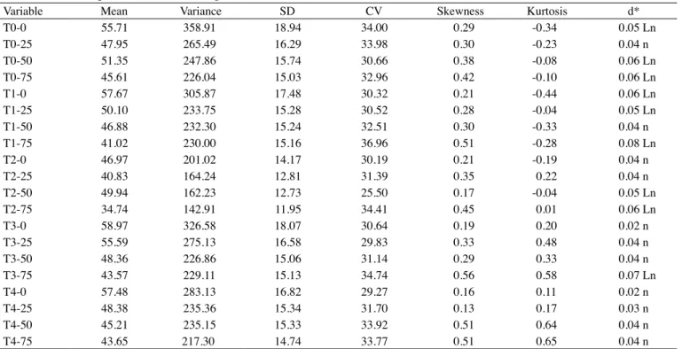
Table 1. Statistical parameters of soil roughness data (mm)
Variable Mean Variance SD CV Skewness Kurtosis d*
T0-0 55.71 358.91 18.94 34.00 0.29 -0.34 0.05 Ln
T0-25 47.95 265.49 16.29 33.98 0.30 -0.23 0.04 n
T0-50 51.35 247.86 15.74 30.66 0.38 -0.08 0.06 Ln
T0-75 45.61 226.04 15.03 32.96 0.42 -0.10 0.06 Ln
T1-0 57.67 305.87 17.48 30.32 0.21 -0.44 0.06 Ln
T1-25 50.10 233.75 15.28 30.52 0.28 -0.04 0.05 Ln
T1-50 46.88 232.30 15.24 32.51 0.30 -0.33 0.04 n
T1-75 41.02 230.00 15.16 36.96 0.51 -0.28 0.08 Ln
T2-0 46.97 201.02 14.17 30.19 0.21 -0.19 0.04 n
T2-25 40.83 164.24 12.81 31.39 0.35 0.22 0.04 n
T2-50 49.94 162.23 12.73 25.50 0.17 -0.04 0.05 Ln
T2-75 34.74 142.91 11.95 34.41 0.45 0.01 0.06 Ln
T3-0 58.97 326.58 18.07 30.64 0.19 0.20 0.02 n
T3-25 55.59 275.13 16.58 29.83 0.33 0.48 0.04 n
T3-50 48.36 226.86 15.06 31.14 0.29 0.33 0.04 n
T3-75 43.57 229.11 15.13 34.74 0.56 0.58 0.07 Ln
T4-0 57.48 283.13 16.82 29.27 0.16 0.11 0.02 n
T4-25 48.38 235.36 15.34 31.70 0.13 0.17 0.03 n
T4-50 45.21 235.15 15.33 33.92 0.51 0.64 0.04 n
T4-75 43.65 217.30 14.74 33.77 0.51 0.65 0.04 n
SD: standard deviation; CV: coefficient of variation; d: normality of the date for test of Kolmogorov-Smirnov (* P < 0.05); Ln:
Log-normal; n: normal.
Table 2. Geostatistical parameters
Variable Model C0 C0+C1 a SD RR
T0-0 Spherical 0.00 375.20 65.33 0.00 189.22
T0-25 Spherical 0.00 282.28 66.29 0.00 162.74
T0-50 Spherical 0.00 263.30 68.77 0.00 157.24
T0-75 Spherical 0.00 238.97 62.93 0.00 150.16
T1-0 Spherical 71.00 314.00 61.00 22.61 174.67
T1-25 Spherical 117.00 246.00 68.00 47.56 152.70
T1-50 Spherical 54.00 250.00 71.00 21.60 152.22
T1-75 Spherical 2.29 240.71 60.66 0.95 151.47
T2-0 Spherical 48.02 208.85 66.39 22.99 141.61
T2-25 Spherical 43.53 176.30 65.15 24.69 128.00
T2-50 Spherical 2.43 172.21 63.76 1.41 127.21
T2-75 Spherical 23.74 144.26 61.52 16.45 119.40
T3-0 Spherical 32.08 328.04 64.85 9.78 180.49
T3-25 Spherical 0.00 262.00 62.00 0.00 165.66
T3-50 Spherical 41.19 228.36 75.11 18.04 150.43
T3-75 Spherical 38.85 219.44 75.39 17.70 151.17
T4-0 Spherical 17.82 258.62 65.12 6.89 168.05
T4-25 Spherical 35.82 227.63 78.58 15.74 153.22
T4-50 Spherical 20.47 222.06 70.78 9.22 153.16
T4-75 Spherical 32.54 206.24 75.71 15.78 147.23
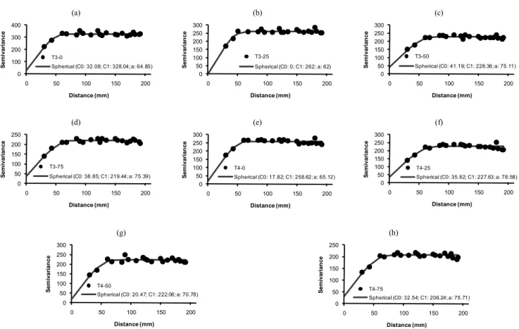
The parameters of the models fitted to the semivariograms are shown in table 2. All semivariograms were fitted to spherical model, confirming this model as the one of the useful for parameters of soil and plant (CAmBArdellA et al., 1994; souzA et al., 2001; siqueirA et al., 2008). The fact that in this study all the data have been fitted to spherical model, confirms that although there have been changes in soil surface roughness caused by the different amounts of simulated rain, it was not detected changes in spatial variability pattern, according to pAzgonzález et al. (1998) and BertolAni et al. (2000).
The treatment without crop residue (T0-0) showed the lowest values of nugget effect (C0, Table 2), while in other treatments the values of C0 vary when the residue amount and rain volume is increased. Values
of nugget effect (C0) near to 0 indicate that the spatial variability at short distance has been detected; therefore it is an indicator of the experiment accuracy as reported by VieirA (2000) and siqueirA et al. (2008). All treatments
showed well defined sill values (C0 + C1, Table 2 and Figure 1 and 2). The analysis of Figure 1 and 2 confirms the hypothesis that the spatial variability pattern has not changed even after the application of simulated rainfall.
The analysis of the semivariograms (Figure 1 and 2) and scaled semivariograms (Figure 3) allows that even occurring specific changes between the values of C0 and C0 + C1 the distribution of semivariance pairs after each of the rain events remains unchanged, the largest differences are caused by soil surface sealing
Figure 1. Experimental semivariograms along with the corresponding fitted models for the studied variables: a) T0-0, b) T0-25,
c) T0-50, d) T0-75, e) T1-0, f) T1-25, g) T1-50, h) T1-75, i) T2-0, j) T2-25, k) T2-50, l) T2-75; T0 - without crop residue; T1 and
T2 = 1 Mg ha-1 and 2 Mg ha-1 with incorporation of maize crop residue; and test of simulated rain (0 mm, 25 mm, 50 mm and
75 mm). Figures are presented for the adjustment of the semivariogram model and their respective values of nugget effect (C0),
structural variance (C1) and range (a).
(a) 0 100 200 300 400 500
0 50 100 150 200
S e m iv a ri a n c e Distance (mm) T0-0
Spherical (C0: 0; C1: 375.20; a: 65.33)
(b) 0 50 100 150 200 250 300 350
0 50 100 150 200
S e m iv a ri a n c e Distance (mm) T0-25
Spherical (C0: 0; C1: 282.28; a: 66.29)
(c) 0 50 100 150 200 250 300
0 50 100 150 200
S e m iv a ri a n c e Distance (mm) T0-50
Spherical (C0: 0; C1: 263.30; a: 68.77)
(d) 0 50 100 150 200 250 300
0 50 100 150 200
S e m iv a ri a n c e Distance (mm) T0-75
Spherical (C0: 0; C1: 238.97; a: 62.93)
(e) 0 100 200 300 400
0 50 100 150 200
S e m iv a ri a n c e Distance (mm) T1-0
Spherical (C0: 71; C1: 314; a: 61)
(f) 0 50 100 150 200 250 300
0 50 100 150 200
S e m iv a ri a n c e Distance (mm) T1-25
Spherical (C0: 117; C1: 246; a: 68)
(g) 0 50 100 150 200 250 300
0 50 100 150 200
S e m iv a ri a n c e Distance (mm) T1-50
Spherical (C0: 54; C1: 250; a: 71)
(h) 0 50 100 150 200 250 300
0 50 100 150 200
s e m iv a ri a n c e Distance (mm) T1-75
Spherical (C0: 2.29; C1: 240.71; a: 60.66)
(i) 0 50 100 150 200 250
0 50 100 150 200
S e m iv a ri a n c e Distance (mm) T2-0
Spherical (C0: 48.02; C1: 208.85; a: 66.39)
(j) 0 50 100 150 200 250
0 50 100 150 200
S e m iv a ri a n c e Distance (mm) T2-25
Spherical (C0: 43-53; C1: 176.30; a: 65.15)
(k) 0 50 100 150 200
0 50 100 150 200
S e m iv a ri a n c e Distance (mm) T2-50
Spherical (C0: 2.43; C1: 172.21; a: 63.76)
(l) 0 40 80 120 160 200
0 50 100 150 200
S e m iv a ri a n c e Distance (mm) T2-75
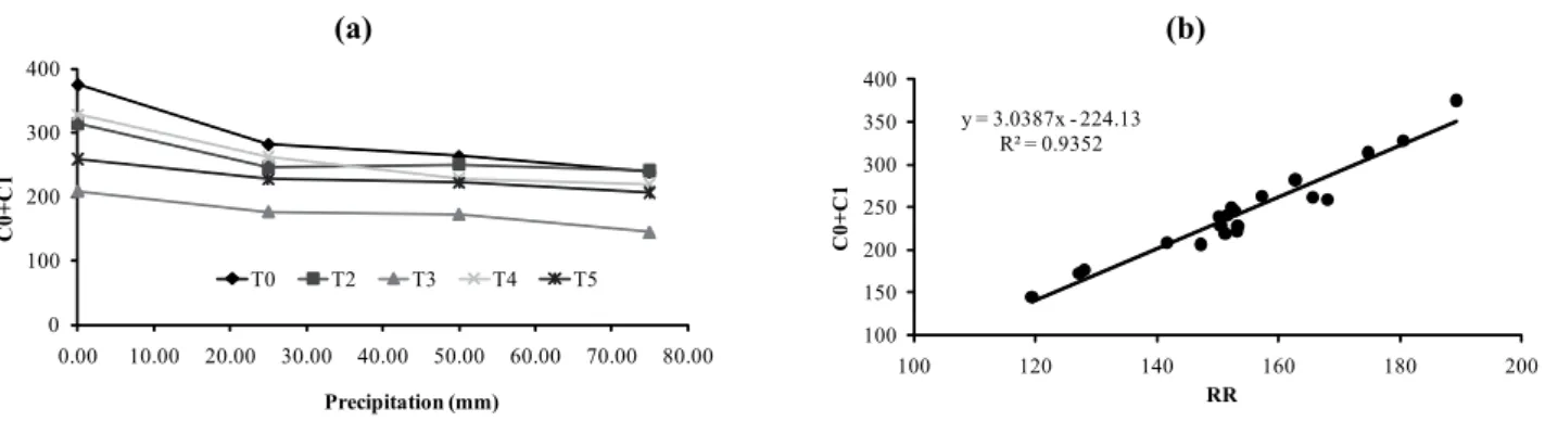
and rill formation during the water erosion process as described by dArBoux et al. (2002) and VidAl Vázquez et al. (2007). This fact can be observed in Figure 4a, which shows a value reduction of sill (C0 + C1) when the rainfall height (mm) increases. The largest variation between the values of C0 + C1 and rainfall (mm) occurs in the treatment without residue (T0) where the reduction of sill with simulated rain is around 36.30%. In other treatments the reduction was 33.10% (T3), 30.92% (T2), 23.34% (T1) and 20.25% (T4).
The values of the range (a) show that in all treatments, the radius of the spatial variability is around 67 mm, indicating that the spacing between measures could be expanded until distances smaller than the radius of spatial variability, without problems for the adequate description of data spatial variability (VieirA, 2000; souzA et al., 2001; siqueirA et al., 2008). On the other hand, we can say that the greatest differences between the values of range (Table 2 and Figure 1 and 2) for the studied treatments are derived from the distribution and sizes of soil aggregates, and the crop residue amount in the case if the crop residue is used, as reported by pAz
gonzález et al. (1998).
The spatial dependence (SD, Table 2) is strong for all treatments except for T1-25 that shows moderate spatial dependence between samples. The scaled semivariogram according to VieirA et al. (1997) allows comparisons of the attributes of different magnitudes. Thus, it is possible to examine the influence of the crop residue and separate rain on the spatial variability of each of the treatments. Analyzing the scaled semivariogram (Figure 3) it appears that the semivariogram for T1-25 shows a different behavior when compared to the others, thus explaining the presence of moderate spatial dependence for this attribute. This fact could be caused by reorganization of aggregates of soil after the first application of simulated rain (25 mm h-1), contributing to have a difference in spatial variability mainly in short distance.
The index of random roughness (RR, Table 2) is considered high for all treatments and areas according to the scale of values of roughness proposed by renArd et al. (1997) for RUSLE (Revised Universal Soil Loss Equation). Bertol et al. (2007) studying the surface roughness of a Cambisol in La Coruña with crop residue amounts up to 8 Mg ha-1 found medium values of random roughness. The presence of high value for (a) 0 100 200 300 400
0 50 100 150 200
S e m iv a ri a n c e Distance (mm) T3-0
Spherical (C0: 32.08; C1: 328.04; a: 64.85)
(b) 0 50 100 150 200 250 300
0 50 100 150 200
S e m iv a ri a n c e Distance (mm) T3-25
Spherical (C0: 0; C1: 262; a: 62)
(c) 0 50 100 150 200 250 300
0 50 100 150 200
S e m iv a ri a n c e Distance (mm) T3-50
Spherical (C0: 41.19; C1: 228.36; a: 75.11)
(d) 0 50 100 150 200 250
0 50 100 150 200
S e m iv a ri a n c e Distance (mm) T3-75
Spherical (C0: 38.85; C1: 219.44; a: 75.39)
(e) 0 50 100 150 200 250 300
0 50 100 150 200
S e m iv a ri a n c e Distance (mm) T4-0
Spherical (C0: 17.82; C1: 258.62; a: 65.12)
(f) 0 50 100 150 200 250 300
0 50 100 150 200
S e m iv a ri a n c e Distance (mm) T4-25
Spherical (C0: 35.82; C1: 227.63; a: 78.58)
(g) 0 50 100 150 200 250 300
0 50 100 150 200
S e m iv a ri a n c e Distance (mm) T4-50
Spherical (C0: 20.47; C1: 222.06; a: 70.78)
(h) 0 50 100 150 200 250
0 50 100 150 200
S e m iv a ri a n c e Distance (mm) T4-75
Spherical (C0: 32.54; C1: 206.24; a: 75.71)
Figure 2. Experimental semivariograms along with the corresponding fitted models for the studied variables: a) T3-0, b) T3-25, c)
T3-50, d) T3-75, e) T4-0, f) T4-25, g) T4-50 and h) T4-75. T3 and T4 = 3 Mg ha-1 and 4 Mg ha-1 with incorporation of maize crop
residue respectively and test of simulated rain (0 mm, 25 mm, 50 mm and 75 mm). Figures are presented for the adjustment of
Figure 3. Scaled semivariograms for the soil surface roughness evaluated: T0 (in a) - without crop residue; T1 (in b), T2 (in c), T3 (in
d) and T4 (in e) - 1 Mg ha-1, 2 Mg ha-1, 3 Mg ha-1 and 4 Mg ha-1 with incorporation of maize crop residue; and test of simulated
rain (0 mm, 25 mm, 50 mm and 75 mm).
(a)
0 0.2 0.4 0.6 0.8 1 1.2 1.4
0 50 100 150 200
S
em
iv
a
ri
a
n
ce
Distance (m)
T0 T0-25 T0-50 T0-75
(b)
0 0.2 0.4 0.6 0.8 1 1.2 1.4
0 50 100 150 200
S
em
iv
a
ri
a
n
ce
Distance (m)
T1 T1-25 T1-50 T1-75
(c)
0 0.2 0.4 0.6 0.8 1 1.2 1.4
0 50 100 150 200
S
em
iv
a
ri
a
n
ce
Distance (m)
T2 T2-25 T2-50 T2-75
(d)
0 0.2 0.4 0.6 0.8 1 1.2
0 50 100 150 200
S
em
iv
a
ri
a
n
ce
Distance (m)
T3 T3-25 T3-50 T3-75
(e)
0 0.2 0.4 0.6 0.8 1 1.2
0 50 100 150 200
S
em
iv
a
ri
a
n
ce
Distance (m)
T4 T4-25 T4-50 T4-75
Figure 4. Variation of sill with rainfall (a) and relationship between random roughness index RR and sill (b) for the surface
roughness of the soil evaluated: T0 - without crop residue; T1, T2, T3 and T4 - 1 Mg ha-1, 2 Mg ha-1, 3 Mg ha-1 and 4 Mg ha-1 with
incorporation of maize crop residue; and test of simulated rain (0 mm, 25 mm, 50 mm and 75 mm).
(a)
0 100 200 300 400
0.00 10.00 20.00 30.00 40.00 50.00 60.00 70.00 80.00
C
0
+
C
1
Precipitation (mm)
T0 T2 T3 T4 T5
(b)
y = 3.0387x - 224.13 R² = 0.9352
100 150 200 250 300 350 400
100 120 140 160 180 200
C
0
+
C
1
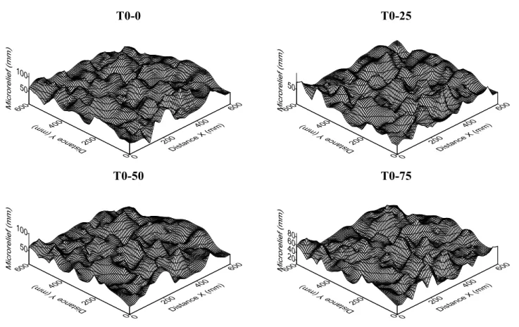
Figure 5. Three-dimensional maps of the surface roughness for the treatments without crop residue (T0) and with successive rainfall events which bring about cumulative 0 mm (T0-0), 25 mm (T0-25), 50 mm (T0-50) and 75 mm (T0-75).
T0-0
T0-25
T0-50
T0-75
Figure 6. Three-dimensional maps of the surface roughness for the treatment 1 Mg ha-1 crop residue (T1) and with successive
rainfall events which bring about cumulative 0 mm (T1-0), 25 mm (T1-25), 50 mm (T1-50) and 75 mm (T1-75).
T1-0
T1-25
T2-0
T2-25
T2-50
T2-75
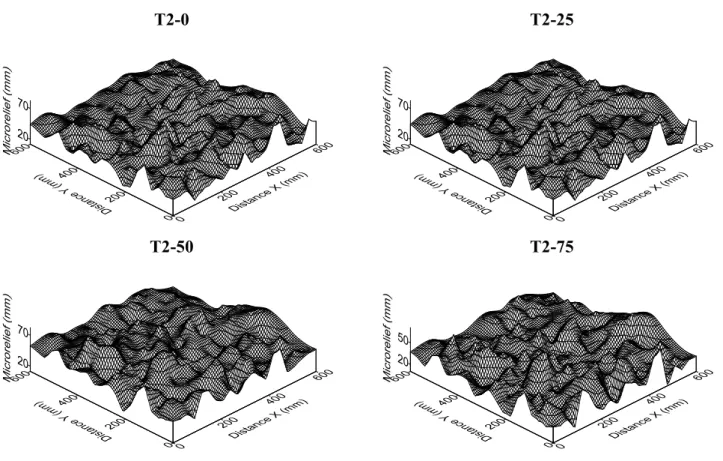
Figure 7. Three-dimensional maps of the surface roughness for the treatment 2 Mg ha-1 crop residue (T2) and with successive
rainfall events which bring about cumulative 0 mm (T2-0), 25 mm (T2-25), 50 mm (T2-50) and 75 mm (T2-75).
Figure 8. Three-dimensional maps of the surface roughness for the treatment 3 Mg ha-1 crop residue (T3) and with successive
rainfall events which bring about cumulative 0 mm (T3-0), 25 mm (T3-25), 50 mm (T3-50) and 75 mm (T3-75).
T3-0 T3-25
RR is justified because the soil preparation generated micro depressions of large dimensions.
The highest value of random roughness (RR) before the first rain test has been found for treatment without crop residue (T0, 189.216 mm), followed by T3 (180.492 mm), T1 (174.674 mm), T4 (168.055 mm) and T2 (141.606 mm). In all treatments after the first rain test there was a reduction in values of RR, according to the results found by other researchers (CAstro et al., 2006; Bertol et al., 2007; VidAlVázquez et al., 2007). For the treatment without crop residue (T0) there was a decrease in roughness of around 40 mm during the process of surface evolution after simulated rain test. In other treatments there was a minor reduction of the soil roughness (from 20 mm to 30 mm), influenced by the action of crop residues that favour the conservation of surface microrelief, during the water erosion process (KAmpHorst et al., 2000; dArBoux et al., 2002; CAstro et al., 2006). The treatment with the highest amount of crop residue (T4) showed the smallest reduction in random roughness index after the simulated rain test, demonstrating the efficiency of crop residues to conservation of soil roughness (Bertol et al., 2007).
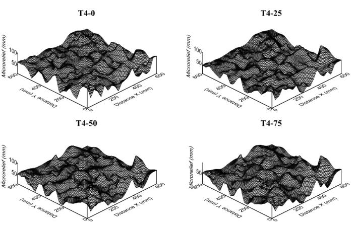
Figure 9. Three-dimensional maps of the surface roughness for treatment 4 Mg ha-1 crop residue (T4) and with successive rainfall
events which bring about cumulative 0 mm (T4-0), 25 mm (T4-25), 50 mm (T4-50) and 75 mm (T4-75).
T4-0 T4-25
T4-50 T4-75
The Figure 4b shows the correlation between the values of the random roughness index (RR) and sill values (C0 + C1). There is a high linear correlation between RR and sill with a R2 = 0.935. However, we must be careful with the interpretation of this correlation, since it is valid for semivariograms with well defined sill, where the values of semivariance increase when the distance of separation between pairs of semivariance increases, stabilizing near the data variance value (VieirA, 2000). There are situations where the semivariance value increases without limits, without a well defined sill, indicating the presence of trends and lack of stationarity (trAngmAr et al., 1987; VieirA et al., 2002).
The presence of stationary data allows an experiment to be repeated, because in this case all samples belong to the same population (VieirA, 2000;
4. CONCLUSIONS
1. The reduction of random roughness (RR), after the events of simulated rain is influenced by the amount of crop residue used in the soil preparation, since residue cover maintains the soil structure.
2. The control treatment, T0 (without crop residue), showed the lowest values of nugget effect (C0), which means the smallest space discontinuity for the used treatments.
3. All the experimental semivariograms were fitted to spherical models before and after simulated rain, indicating that changes in surface roughness had no bearing in the spatial variability pattern.
4. The range (a) of spatial dependence showed a tendency to decrease with the increase of accumulated rain water which was more evident in treatments with less residue cover (0, 1 and 2 Mg ha-1).
ACKNOWLEDGEMENTS
The authors are grateful to the Ministerio de Asuntos Exteriores y de Cooperación (MAEC-AECID) from Spain by the granting of scholarships for PhD studies. This work has been funded by Ministerio de Educación y Ciencia, within the framework of research project CGL2005-08219-HID, co-funded by the Galician government Xunta de Galicia, within the framework of research project PGIDIT06PXIC291062PN and by the European Regional Development Fund (ERDF).
REFERENCES
ALLMARAS, R.R.; BURWELL, R.E.; LARSON, W.E.; HOLT,
R.F. Total porosity and randon roughness of the interrow zone
as influenced by tillage. USA, Conservation Research Report, v.7, p.1-14, 1966.
BERTOL, I.; AMARAL, A.J.; VIDAL VÁZQUEZ, E.; PAZ GONZÁLEZ, A.; BARBOSA, F.T.; BRIGNONI, L.F. Relações
da rugosidade superficial do solo com o volume de chuva e
com a estabilidade de agregados em água. Revista Brasileira
de Ciência do Solo, v.30, p.543-553, 2006.
BERTOL, I.; PAZ GONZÁLEZ, A.; VIDAL VÁZQUEZ, E.
Rugosidade superficial do solo sob diferentes doses de resíduo
de milho submetido à chuva simulada. Pesquisa Agropecuária
Brasileira, v.42, p.103-110, 2007.
BERTOLANI, F.C.; PAZ GONZÁLEZ, A.; LADO LIÑARES, M.; VIDAL VÁZQUEZ, E.; MIRANDA, J.G.V. Variabilidade espacial
da rugosidade superficial do solo medida com rugosímetros de
agulhas e laser. Bragantia, v.59, p.227-234, 2000.
CAMBARDELLA, C.A.; MOORMAN, T.B.; NOVAK, J.M. Field-scale variability of soil properties in central Iowa soils.
Soil Science Society of America Journal, v.58, p.1501-1511, 1994.
CASTRO, L.G.; COGO, N.P.; VOLK, L.B.S. Alterações na
rugosidade superficial do solo pelo preparo e pela chuva e sua relação com a erosão hídrica. Revista Brasileira de Ciência do
Solo, v.30, p.339-352, 2006.
CURRENCE, H.D.; LOVELY, W.G. The analysis of soil surface
roughness. Transactions of the ASAE v.13, p.710-714, 1970.
DARBOUX, F.; GASCUEL-ODOUX, C.; DAVY, P. Effects of
surface water storage by soil roughness on overland-flow
generation. Earth Surface Processes and Landforms, v.27,
p.223-233, 2002.
ELTZ, F.L.; NORTON, L.D. Surface roughness changes as affected by rainfall erosivity, tillage, and canopy cover. Soil Science Society of America Journal, v.61, p.1746-1755, 1997.
FAO. Soil map of the World. Revised Legend. Rome: FAO,
1994.
GOLDEN SOFTWARE. Surfer for windows. Realese 7.0. Contouring and 3D surface mapping for scientist’s engineers: User’s guide. New York: Golden Software, 1999. 619p.
HUANG, C. Quantification of soil microtopography and
surface roughness. In: BAVEYE, P.; PARLANGE, J.Y.;
STEWART, B.A. (Ed.) Fractals in Soil Science. New York: CRC Press, 1998. P.153-168.
HUANG, C.; BRADFORD, J.M. Application of a laser scanner
to quality soil microtopography. Soil Science Society of
America Journal, v.56, p.14-21, 1992.
KAMPHORST, E.C.; JETTEN, V.; GUÉRIF, J.; PITKÄNEN, J.; IVERSEN, B.V.; DOUGLAS, J.T.; PAZ, A. Predicting
depressional storage from soil surface roughness. Soil Science
Society of AmericaJournal, v.64, p.1749-1758, 2000.
NAVAS, A.; ALBERTO, F.; MACHIN, J.; GALAN, A. Design and operation of rainfall simulator for studies of runoff and
soil erosion. Soil Technology, v.3, p.385-397, 1990.
PAZ GONZÁLEZ, A.; MIRANDA, J.G.V.; BERTOLANI, F.C.
Caracterización geoestadística del microrrelieve del suelo a partir de datos obtenidos con rugosímetro láser. In: COLEGIO
OFICIAL DE FÍSICOS (Ed.). Agua. Madrid: Espacios naturales
y Biodiversidad, 1998. p.143-158.
RENARD, K.G.; FOSTER, G.R.; WEESIES, G.A.; McCOOL,
D.K.; YODER, D.C. Predicting soil erosion by water: a
guide to conservation planning with the revised universal
soil loss equation (RUSLE). Washington: U.S. Department of
Agriculture, 1997. 384p. (Agriculture handbook, 703)
SIQUEIRA, G.M.; VIEIRA, S.R.; CEDDIA, M.B. Variabilidade
espacial de atributos físicos do solo determinados por métodos
SOUZA, Z.M.; SILVA, M.L.S.; GUIMARÃES, G.L.; CAMPOS, D.T.S.; CARVALHO, M.P.; PEREIRA, G.T. Variabilidade
espacial de atributos físicos em um Latossolo Vermelho Distroférrico sob semeadura direta em Selvíria (MS). Revista Brasileira de Ciência do Solo, v.25, p.699-707, 2001.
TRANGMAR, B.B.; YOST, R.S.; WADE, M.K.; UEHARA, G.;
SUDJADI, M. Spatial variation of soil properties and yield
on recently cleared land. Soil Science Society of America
Journal, v.51, p.668-674, 1987.
VIDAL VÁZQUEZ, E.; MIRANDA, J.G.V.; PAZ GONZÁLEZ, A. Describing soil surface microrelief by crossover length and
fractal dimension. Nonlinear Processes in Geophysics, v.14,
p.223-235, 2007.
VIEIRA, S.R. Geoestatística em estudos de variabilidade
espacial do solo. In: NOVAIS, R.F.; ÁLVAREZ, V.H.;
SCHAEFER, G.R. (Ed.). Tópicos em Ciência do Solo. Viçosa:
Sociedade Brasileira de Ciência do Solo, 2000. v.1, p. 1-54.
VIEIRA, S.R.; MILLETE, J.; TOPP, G.C.; REYNOLDS, W.D.
Handbook for geoestatistical analysis of variability in soil and climate data. In: ALVAREZ, V.V.H.; SCHAEFER, C.E.G.R.;
BARROS, N.F.; MELLO, J.W.V.; COSTA, J.M. Tópicos em Ciência do Solo. Viçosa: Sociedade Brasileira de Ciência do Solo, 2002. v.2, p.1-45.
VIEIRA, S.R.; TILLOTSON, P.M.; BIGGAR, J.W.; NIELSEN,
D.R. Scaling of semivariograms and the kriging estimation of
field-measured properties. Revista Brasileira de Ciência do