MULTIPARAMETER CORRECTION INTENSITY OF TERRESTRIAL LASER
SCANNING DATA AS AN INPUT FOR ROCK SURFACE MODELLING
V. Paleček* a, P. Kubíček b,
Laboratory on Geoinformatics and Cartography, Masaryk University, Kotlářská 2, 61137 Brno, Czech Republic a([email protected]) b([email protected])
Commission III, WG III/2
KEY WORDS: Terrestrial laser scanning, Rock formations, Filtration, Spectral information, Correction, Intensity
ABSTRACT:
A large increase in the creation of 3D models of objects all around us can be observed in the last few years; thanks to the help of the rapid development of new advanced technologies for spatial data collection and robust software tools. A new commercially available airborne laser scanning data in Czech Republic, provided in the form of the Digital terrain model of the fifth generation as irregularly spaced points, enable locating the majority of rock formations. However, the positional and height accuracy of this type of landforms can reach huge errors in some cases. Therefore, it is necessary to start mapping using terrestrial laser scanning with the possibility of adding a point cloud data derived from ground or aerial photogrammetry. Intensity correction and noise removal is usually based on the distance between measured objects and the laser scanner, the incidence angle of the beam or on the radiometric and topographic characteristics of measured objects. This contribution represents the major undesirable effects that affect the quality of acquisition and processing of laser scanning data. Likewise there is introduced solutions to some of these problems.
1. INTRODUCTION
Nowadays, we can observe in the field of acquiring topographical data wide variety of possible systems and methods of their use. Except for traditional tachymetry we can meet with classical terrestrial and aerial photogrammetry, processing systems, image by image correlation method Structure from Motion (SFM) and various laser scanning systems (Gross and Pfister, 2007). These systems differ in the way of collecting spatial data, processing or time component acquisition. This is a selective and non-contact collecting of information which is often connected with technological properties of devices. In the present, the basic processing output is known as a point cloud formed by the plurality of points defined by the triplets X, Y and Z coordinates. Often these points carry further information measured by the sensor, such as a combination of RGB values, the intensity of the reflection beam and others. It is also necessary to realize that each point cloud has a timestamp at the time of the acquisition, which allows to study the temporal changes in the landscape (Shan and Toth, 2008), and therefore in this context we can speak about 4D space. Based on this information entering data goes into other processing techniques which are aimed often to create accurate 3D models of objects. Especially in the inventory in construction are therefore often required only geometric information captured scene and vice versa modelling is using spectral information about the objects and also it is only used for mapping of damage stability or quality of materials (Mills and Fotopoulos, 2015). The situation is different in the current natural environment which often occurs greater heterogeneity of objects whose geometry almost disrespect the various geometric primitives which are being used in architecture or engineering. In such situations, it is necessary to distinguish between different objects by using appropriate set of procedures which are exploiting the higher rate of spectral information objects (Kashani et al., 2015) which were measured before.
* Corresponding author
In the field of terrestrial laser scanning which is performed with help of a static location scanner you can meet smaller space missions that correct/refill information such as mobile scanning devices. Often it is a qualitatively less powerful devices in comparison with airborne scanners which are used primarily indoors or outdoors on a short distance of a few tens of meters and also often for registering particularly single reflection (Shan and Toth, 2008). But there are exceptions of the possibility of measuring several hundred meters and simultaneously it depends on ideal reflective properties of the measured objects (Kashani et al., 2015).
As an example of mapping and modelling the rocky object in 3D we can mention the use of terrestrial laser scanner for refining the position and altitude information, as the representative of relatively complicated natural structure, in which you can not only use the geometry of the object, unless you want to lose part of the recorded information.
The main aim of this article is in particular:
- Presentation of the known parameters and processes of correction signals, which are used in ideal situations
- Performance issues at the stage of data collection and processing, to which everyone faces
- Demonstration of solutions to some problems of laser processing data on the selected point cloud
2. PARAMETERS AND PROCESSES OF CORRECTION SIGNALS
The principle of measuring distances using a laser beam is generally known. The rectified laser beam after its reflection
from the object is recorded on the detector and the measured time and the return intensity. Except of not so far often used records of return full waveform in ground missions where are widely used primarily pulse and the phase method of measurement (Shan and Toth, 2008).
Rectified beam loses its original intensity immediately after leaving the facility, but there are many other influences that weaken the beam. Some of them can be measured and corrected. Some can be measured only indicative and approximate. Last group is performed by others which are random in nature and can be removed very difficultly. All of these effects could be divided into four groups according to their origin (Kaasalainen et al., 2011):
1) Parameters of the scanner (range of measured values, weak signal amplification, noise reduction ...)
2) Atmospheric effects (scattered, absorbed, reflected radiation depending on temperature and air pressure, humidity, quantity of aerosols ...)
3) Properties of the measured objects (geometric properties, chemical and physical properties)
4) Acquisition geometry (object distance, the angle of dispatch and incidence of the laser beam)
During normal terrestrial scanning we can work practically only with the properties of measurement objects and acquisition geometry, while the parameters of the scanner are determined by calibration of the device by its manufacturer. Atmospheric effects can be only approximated on the basis of several measurements indicative nearby scanning. For calculating the actual value of the reflected energy was introduced a general relationship (Höfle and Pfeifer, 2007)
= ρcos � � �
(1)
where: = the received laser power
= the function of the transmitted power = the receiver aperture diameter ρ= the target reflectance
= the incidence angle
�= the system transmission factor
� �= the atmospheric transmission factor
As the conditions of scanner settings during the mission does not change, it is possible to consider this folder as a constant. In the case that the scanning takes place in the outdoor dynamically changing conditions where the request is not the highest quality and the range scan then it is possible to consider an atmospheric effects as constant (Tan et al., 2016). However, if the high spatial resolution of the scanning, accuracy and range of spherical is required, the entire scanning process may take a long time and in order to it is also necessary to consider these influences. Most often it is carried out with the correction of the angle of incidence, distance, and reflectivity of the subject, which is given by the sum of geometric, physical and chemical properties. To these just mentioned parameters will be dedicated the following chapters.
2.1 Acquisition geometry
Correction of the length and the angle of incidence in this group result from the relative position and orientation of the scanning unit and the measuring object.
Linear factor plays attenuating part because of the transmitted beam is facing in its passage through the atmosphere absorption, reflection and diffraction, which is caused by air molecules and the various aerosols contained inside. At the same time beam must face all of these effects twice, because of travelling signals to and than back into the detection device in scanner from the object. The theoretical model attenuation dispatched beam to two different reflective objects can be observed in Fig. 1a.
The incidence angle is partially object properties because the defining of local plane is based on the surface structure. There is also very important the direction of transmission beam, which determines together with the local plane an incident angle θ. The size of this angle is calculated based on the normal vector which is derived thanks to interlay several neighbouring points of the plane and the vector obtained by coordinate difference between the measured point and the origin of the coordinate system represented by placing the scanner. The power of intensity attenuation on incidence of Lambert surface equals to cos (Kaasalainen et al., 2009). The theoretical model based on the attenuation of incident angle for two different reflective objects is depicted in Fig. 1b.
Figure 1. Theoretical model of beam attenuation by the distance (a) and the angle of incidence (b) for two diffusely reflecting surfaces (� = 0, �) (Kashani et. Al, 2015).
2.2 Properties of the measured objects
Reflectance ratio determines the amount of reflected and incident radiation from the surface of an object of a certain wavelength which may vary in time. It is also a decisive parameter, which allows to distinguish between different types of objects (Shan and Toth, 2008). The reflectance of the object is determined primarily by its chemical composition, but its amount varies depending on the dynamic physical influences such as moisture or body temperature. For example, using the short infrared radiation, a high humidity causes, that much of the energy of the laser beam will be absorbed and detecting device of scanner will not reach a
sufficiently large amount of radiation to be given pulse measured (Kashani et al., 2015). On the contrary, a higher temperature of the object may cause increase of intensity of the reflected signal, which in turn distorts the true spectral characteristics of the object (Penghe, 2011). The spectral behavior of different types of objects can be measured by a spectrometer or can be found in spectral libraries resulting efforts USGS (United States Geological Survey) or as output from ASTER (Advanced Spaceborne Thermal Emission and Reflection Radiometer), which includes data from the libraries of the Johns Hopkins University (JHU) Spectral Library, the Jet Propulsion Laboratory (JPL) Spectral Library and the United States Geological Survey (USGS - Reston) Spectral Library.
An important property of objects is their surface roughness. This is always expressed as the ratio of the average size of the individual grains of the material from which the object is composed and the size of the orthogonal projection of the laser beam spot on the surface of the subject (Pesci and Teza, 2008). From this perspective, we distinguish two types of surfaces. The surface in which is average size of unevenness in comparison with the width of the laser spot very small, becomes absolutely rough and is called as Lambertian surface. From this surface the incident beam is reflected at reduced intensity in all directions (diffuse reflection). The opposite is absolutely smooth surface that reflects the beam in the same plane and at the same angle at which a beam reaches it (mirror reflection). While in the urban environment we can meet mirror reflection quite often, the common ones in the nature are diffuse reflectors despite the fact that their surface is not absolutely rough (Pesci and Teza, 2008). The size of the laser spot depends on the divergence of the beam and the distance of the object. The greater the divergence or distance, the wider will be the projection of the laser beam. Therefore an identical object from two different measured distances may seem like a relatively smooth one, and in the second case as a relatively rough.
3. PERFORMANCE ISSUES AT THE STAGE OF DATA COLLECTION AND PROCESSING
As it was already indicated in the introductory chapter, some effects could be modelled using various corrections and some only guess with higher or lower degree of reliability. The requirement for each processing of point clouds is the highest possible degree of automation, speed and of course accuracy. Unfortunately, various theoretical models of the effects may not be valid unconditionally and they are often compared with the empirical observation that contains from theoretical model of a certain degree of distortion. Examples of comparison of some theoretical models and empirical observations can be found in Kashani et al., 2015. This chapter presents some problems of theoretical modelling of the above factors and examples of their solutions based on the acquired point clouds. This cloud was produced by terrestrial laser scanner Faro Focus3D 120 and created by combining nine separate scans to map the perimeter walls of the selected rock formation, the preview can be seen in Fig. 2.
Figure 2. A preview from the source point clouds.
3.1 Distance effects correction
If beam intensity attenuation due to distance can be expected as a function shown in Fig. 1a, various studies (Blaskow and Schneider, 2014 or Tan et al., 2016) however, showed that this function is modified by some manufacturers of the scanners due to the automatic disproportionate amplification of weak signals from distant or low reflective objects. Diffuse solar radiation or multipath, which increase the proportion of noise may be the true reason for this amplification. At the same time you can meet with the partial attenuation of high intensity, which is caused by the saturation of detecting device by reflected beams from the nearby and very reflective objects, so instead of a relatively simple theoretical model we meet with polynomial functions of higher orders, which at first glance contradicts the laws of physics (Tan et al., 2016). This function � ) can be rarely reached from manufacturers of these laser scanners, and therefore for our own correction data must be calculated based on the revised formula (1), which presented Tan et al., 2016.
� = ρcos ∑( � �)
�
�=
= �/ ∑( � �) �
�=
(2)
where: � = the distance corrected intensity
= the constant parameter ( = � / ) = the degree of the polynomial
�= polynomial coefficients
�= the distance between scanning aperture and
measured points �= the measured intensity
In equation (2) it is assumed that for a given position from which scanning takes place, the elements related to the internal adjustment device are constant, and therefore can be described as constant (but unknown) value C. Further, the parameter , which at greater distances ceases to be relevant for the calculation of the intensity (Kashani et al., 2015), is replaced by a polynomial function of the appropriate order. The measured intensity can be further normalised by the assistance of determination reference distance by � = ∑ (��= � �). Determination of a suitable polynomial plane based on the measurements of the reference object positioned at a known distance is obtained based on the calculation of least-squares adjustment. The exact method of calculation is given in (Tan et al., 2016).
This method requires that before the own missions there should be carried out own measuring the reflectance of a reference objects placed at a known distance and ideally oriented in the direction perpendicular to the incident beam in order to eliminate the influence of weakness defined by angle of incidence. This time-consuming preparation is not ideal, but it is possible to avoid such a process during the processing stage. The solution
may be to provide appropriate function based on the selection of reference points in the captured point cloud. The reference points are those points that belong to the same type of object in the cloud, located on several different places from position of the scanner. These objects must satisfy a presumption of the same physical and chemical properties which guarantee a certain spectral behavior. The last requirement is that the transmitted laser beam would keep a zero angle of incidence that the most of the energy reflects back straight into device detectors. If these reference points are plotted and at the same time uniformly cover a range of distances in which we apply a correction of length, this can interspaced by suitable polynomial function, ideally accompanied by confidence intervals.
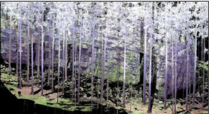
In Fig. 3 can be seen an example of selection of reference points based on scans of tree trunks around the selected rock formation. Here it can be assumed that the reflection conditions are at a given time for one kind of tree constant. Selection of reference points is ensured by establishing points of the same height level as the location of the transmitting laser beam optics, and selecting points for which the condition of zero angle of incidence is the most likely fulfilled. For these reference points may be found suitable polynomial fit, which defines a function for correcting the length. (Fig. 4). Due to this function, it is roughly estimated internal setup and operation of the amplifier on the reflected signal and correct the originally different values of one type of object to values very close despite the fact that different types of objects will likely have a different average value of intensity and different dispersion values.
Figure 3. Sample of selection of reference points.
Figure 4. Polynomial interleaving of reference points and derived equation.
3.2 Angle of incidence correction
Presuming attenuation measured intensity defined functions of the angle of incidence as shown in Fig. 1b. The greater the incident angle, the lower the intensity appears at the detector device. According to some studies (Kaasalainen et al., 2009) this relationship is determined by the values cos , when = 0 °→ cos =1 and for = 90 °→cos =0. Derivation of corrected intensity � of the angle of incidence is then � = �ρ cos . Determination of the angle of incidence can be derived based on knowledge of the normal vector at a given point, and also a knowledge of the size of the vector between the beginning of the scanning system and the observed point. Schematic drawing, which provides Tan and Cheng, 2016 is shown in Fig. 5. According to this scheme, you can calculate the magnitude of and cos using the following formulas (Tan and Cheng, 2016):
= √ − + − + − (3)
cos = | ∗ |�||∗ � (4)
where: , , = coordinates of the point of interest , , = coordinates of the scanner center
= the partial vectors − , − , − �= the normal vector
Figure 5. Schematic drawing of a system for calculating incident angle according to Tan and Cheng, 2016.
While the magnitude of the vector between the beginning of the system and a given point can be detected at the registered point cloud by simple subtraction of X, Y and Z coordinates, the
determination of the normal vector in this regard is more complex. An essential step is to create a local plane, which requires the calculation of at least two other close neighboring points. When objects can have different structures and shapes, it is not appropriate to use this low number of points. While the calculation of directive plane is not too complicated by using the least-squares adjustment, especially important is the selection of an appropriate number of neighboring points, from which the directive counts. In principle it is possible to collect points to define a local plane in three ways. The first way is to define a certain number of nearest points. This can be very misleading, if the points are too far from others. The second method is based on the defining the size around points. This size works for example as a radius of the sphere generated around a given point and all points that are located inside this sphere are then included in the calculation of the local plane. The last method is based on determining the octree level, which is used by those closest neighbors who fall into the relevant cube belonging to selected points (Gross and Pfister, 2007).
When we determine the number of nearest neighbors, we meet at least two kinds of problems, which are the variations in density point field and also in the wrong direction of normal vectors. Fluctuations point density can be observed in Fig. 3. Here is visible a high density of points placed on tree trunks and on the earth's surface in their neighborhood, while the far rock walls show a much lower density. This is given by different shutters for objects that occur too close to device during scanning, and also the actual scanning method which is determined in most devices by the certain angle sweep of the beam to the surroundings. This angle causes that with increasing distance the point spacing increases and thus their density decreases. Thanks to this fact it is very difficult to adjust the size of the neighborhood and the number of nearest neighbors, so that degree of simplification for the calculation of the local plane was in whole point cloud constant. When establishing a small neighborhood of a point, than can happen that for more distant objects will not be found a minimum number of points to calculate a local plane and thus there will not be possible to determine the normals. If we would like to establish a sufficiently large neighborhood to these distant objects, it would mean that on nearby objects a large amount of points for the calculation of local planes entered. This will result in a greater degree of deviation from the actual local surface and also increase the requirements for computational power. A possible solution is the interpolation of original point clouds into a new regular grid, but at the cost of losing the original geometry of objects and thus part of the measured information. The second problem, which in conjunction with the normal vector computation occurs, is the incorrect orientation. For example, for aerial laser scanning is the default direction of the vector surface normal direction determined by used ellipsoid. Terrestrial laser scanning is much more likely to encounter various shapes of objects showing the different orientation of their parts. If we scan for example in the areas of the rock overhangs and thanks for that also a strong decline in the density of points, the software tools detects surfaces badly as a new part from the original surface, so determine the direction of the normal vector in the opposite direction is performed. Disordered structures such as branches and treetops face a similar problem when determining the orientation of the normal vector is almost impossible. In that case, when we can observe a different shadows in point clouds, it is possible to create separate zones where points are in contiguous clusters. For each such surface can be determined normal vectors independently of the other separate clusters, and if necessary turn these vectors in right direction. This approach can also be used in removing problematic clusters for which the determination of the direction of the normal vector
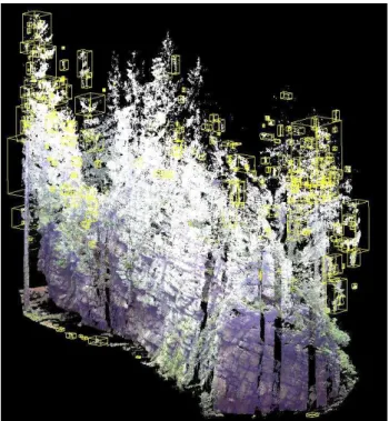
is problematic. Sample applications for the selection of tree crowns in CloudCompare software ver. 2.6.3 depicted in Fig. 6.
Figure 6. Selection of clusters of points belonging to a separate part of the branches and treetops executed in the program CloudCompare ver. 2.6.3.
3.3 Other corrections
Other influences that can be partially solved by corrections are atmospheric influences. These are usually at the aerial laser scanning solved by various atmospheric models for simulating the adjustment of key parameters power beam attenuation. The loss of energy at terrestrial scanning is in most cases negligible, and therefore it is more important the effect of divergence of the beam, which has a particular influence on the geometrical information of modelled objects. With increasing distance from the laser source device, the beam gradually expands and increases diameter, so it would met more likely during his flight some of its fragments number of objects when these objects are too close to the beam direction of flight. The results are a multipath, the reduction ratio of the captured signal to noise, reduction in the density measurements in remote locations and the apparent expansion of remote objects (Vosselman and Maas, 2010). Unfortunately, this problem can not be detected from the captured data, but only by own measurements on real objects.
4. CONCLUSIONS
In this paper we presented major shortcomings and problems in the collection and processing of accurate data acquired by terrestrial laser scanner with a focus on natural objects and also to distortion of the measured intensity of the return beam. Overall there were introduced four groups of causes, which differ in weight and processing capabilities of distorted signal. The effects belonging to the Acquisition geometry have been described by theoretical models and they were compared with observations and processing procedures. While distance correction was observed to modify the signal using a polynomial function, the angle of incidence depends on more parameters. The fundamental problem is to determine the correct approach to determine the size and orientation of the local normal plane of
the object surface. Open question remains in the dealing with divergence of the beam, when some of its consequences can not be captured from measured data and thus can not be correct. In the case of solving all of the significant influences that could be corrected, we should receive corresponding spectral behavior of objects, which could be used for automatic segmentation of different types of objects assuming the use of this information in the existing models of working only with geometric information of point clouds.
REFERENCES
Blaskow, R., and Schneider, D., 2014. Analysis and correction of the dependency between laser scanner intensity values and range. The International Archives of Photogrammetry, Remote Sensing
and Spatial Information Sciences, 40(5), 107-112.
Gross, M. and Pfister, H., 2007. Point-Based Graphics. Morgan Kaufmann Publishers Inc., San Francisco, CA, USA. pp 552.
Höfle, B. and Pfeifer, N., 2007. Correction of laser scanning intensity data: Data and model-driven approaches. ISPRS
Journal of Photogrammetry & Remote Sensing (62), 415-433.
Kaasalainen, S., Jaakkola, A., Kaasalainen, M., Krooks, A. and Kukko, A., 2011. Analysis of Incidence Angle and Distance Effects on Terrestrial Laser Scanner Intensity: Search for Correction Methods. Remote Sensing (3), 2207-2221.
Kaasalainen, S., Vain, A., Krooks, A. and Kukko A., 2009. Topographic and distance effects in laser scanner intensity correction. International Archives of the Photogrammetry,
Remote Sensing and Spatial Information Sciences (38), 219–222.
Kashani, A. G., Olsen, M. J., Parrish, C. E. and Wilson, N., 2015. A Review of LIDAR Radiometric Processing: From Ad Hoc Intensity Correction to Rigorous Radiometric Calibration.
Sensors, 15(11), 28099-28128.
Mills, G. and Fotopoulos, G., 2015. Rock Surface Classification in a Mine Drift Using Multiscale Geometric Features. IEEE
Geoscience and Remote Sensing Letters. 12(6), 1322-1326.
Penghe, Z., 2011. New Applications For Laser Scanning. Infrastructure and Geomatics Research Division, The University of Nottingham, UK
https://www.nottingham.ac.uk/engineering/studentlife/summerr esearchprogramme/documents/posters2011/zhangpenghe.pdf (27. 4. 2016).
Pesci, A. and Teza, G., 2008. Effects of surface irregularities on intensity data from laser scanning: an experimental approach.
Annals of Geophysics (51), 839-848.
Shan, J. and Toth, C. K., 2008. Topographic Laser Ranging and Scanning: Principles and Processing. CRC Press, Boca Raton, FL, USA. pp 590.
Tan, K. and Cheng X., 2016. Correction of Incidence Angle and Distance Effects on TLS Intensity Data Based on Reference Targets. Remote Sensing. 8(3), 251.
Tan, K., Cheng, X., Ding, X. and Zhang, Q., 2016. Intensity Data Correction for the Distance Effect in Terrestrial Laser Scanners. IEEE Journal of Selected Topics in Applied Earth Observations
and Remote Sensing, 9(1), 304-312.
Vosselman, G. and Maas H.G., 2010. Airborne and Terrestrial Laser Scanning. Whittles Publishing, Dunbeath, Scotland, UK. pp 318.