Confinement in the 3-Dimensional Gross-Neveu Model at Finite Temperature
F. C. Khannaa, A. P. C. Malbouissonb, J. M. C. Malbouissonc, and A. E. Santanac,d a Theoretical Physics Institute, University of Alberta, Edmonton
Alberta T6G 2J1, Canada
b CBPF/MCT, Rua Dr. X. Sigaud 150, 22290-180,
Rio de Janeiro, RJ, Brazil
c Instituto de F´ısica, Universidade Federal da Bahia,
40210-340, Salvador, BA, Brazil
d Instituto de F´ısica, Universidade de Bras´ılia, Bras´ılia, DF, Brazil (Received on 18 August, 2006)
We study theN-component (2+1)-dimensional Gross-Neveu model bounded between two parallel planes sep-arated by a distanceLat finite temperature (T). We obtain a closed expression for the large-Neffective coupling constantg=g(L,T,λ). Different behavior depending on the magnitude of the fixed coupling constantλis found to lead to a “critical” valueλc. Ifλ<λc, only short-distance and/or high-temperature asymptotic freedom is found. Forλ≥λcone also observes spatial confinement, which is destroyed by temperature effects. We find a confining length,Lc≃1.61f m, that is close to the proton charge diameter (≈1.74f m) and a deconfining temperature,≃138MeV, which is comparable to the estimated value of≈200MeVfor hadrons.
Keywords: Gross-Neveu model; Four-point function; Spatial confinement
Effective models in quantum field theories have been em-ployed over the last decades in trials to obtain clues about the behavior of strongly interacting particles. Among them, the Gross-Neveu model [1], dealing with the direct four-fermions interaction, has been analyzed at finite temperature as an ef-fective model for QCD and for superconducting systems (see for instance Ref. [2, 3]). Calculation of the effective potential of theφ4theory at finite temperature has also been performed
[4].
Recently, we have studied the N-components tridimen-sional Gross-Neveu model at zero temperature, bounded be-tween two parallel planes [5]. A closed expression was de-rived for the large-Neffective coupling constantg(L,λ)as a function of the distanceLbetween the planes. From this re-sult, the behavior ofg(L,λ)depending on the magnitude of the free space fixed coupling constantλwas found, such that for smallλ, the model presents asymptotic freedom at short distances. On the other hand, for large enough values of λ
both spatial confinement and short distance asymptotic free-dom are simultaneously present. In this context, the analysis of the effect of temperature is crucial, since it affects the con-finement properties. The main objective of the present Letter is to study the spatial confinement and thermal deconfinement properties of the Gross-Neveu model.
We recall that even though it is perturbatively non-renormalizable for dimensions D>2, the massive Gross-Neveu model in Euclidean tridimensional (3-D) space has been shown to exist and has been explicitly constructed in the large-N [6]. A decisive physical point that brings con-sistency to this derivation is a theoretical result [7] supporting the idea that perturbatively non-renormalizable models do ex-ist and have a physical meaning. For theN=1 case, some op-erators can be made more relevant in the low energy region if the fermionic field is minimally coupled to the Chern-Simons field [8, 9].
We consider the N-component 3-D massive Gross-Neveu model, in the large-Nlimit, compactified along the imaginary-time axis and also along one of the spatial directions. From a
physical point of view, in terms of a generalized Matsubara formalism [10], the model is intended to describe fermions bounded between two parallel planes, a distanceLapart from one another and in thermal equilibrium with a reservoir at tem-peratureT =β−1. From the four-point function, we define
an effective renormalized coupling constantg(L,β,λ)in the large-Nlimit, which presents different behavior withLandβ
if the fixed coupling constantλis below or above some “criti-cal” valueλc: high-T and short-distance asymptotic freedom, ifλ<λc; withλ≥λc, we obtain simultaneously asymptotic freedom and spatial confinement, for low enough tempera-tures. As the temperature is increased, a deconfining transi-tion occurs. This is the first time, to our knowledge, that such an analytical calculation has been performed for an effective ab initiomodel.
Considering the Gross-Neveu model as an effective theory for the strong interaction between quarks and taking the con-stituent quark mass (m≈350MeV) as the fermion mass, we find a confining length of 1.61f mwhich is close to the proton charge diameter of≈1.74f m. Also, the temperature destroy-ing the confinement, 138MeV, is comparable to the estimated deconfinement temperature for hadrons (≈200MeV).
in films, wires and grains [12]; for the Casimir effect for bosons [13] and for fermions in a box [14]; and, in partic-ular, for the Gross-Neveu model at zero temperature [5]. It is worth emphasizing that for the fermionic field, the bound-ary (anti-periodic) conditions coincide with the physical bag-model conditions [5, 15, 16].
Our starting point is the Wick-ordered massive Gross-Neveu Lagrangian in aD-dimensional Euclidean space,
L
=: ¯ψ(x)(i6∇+m)ψ(x):+u2(: ¯ψ(x)ψ(x):)
2,
(1) wheremis the mass,uis the coupling constant,xis a point of
RDand theγ’s are either 2×2 or 4×4 matrices. The quantity ψ(x)is a spin 12 field havingN (flavor) components, ψa(x), a=1,2, ...,N. Summation over flavor and spin indexes is understood. Here we consider the large-N limit (N →∞), which permits considerable simplification. We use natural units,~=c=kB=1.
We consider the system bounded between two parallel planes, normal to one of the spatial axis, a distanceL apart from one another and in thermal equilibrium with a reser-voir at temperature T =β−1. We work with Cartesian
co-ordinates x= (x0,x1,z), where x0 corresponds to the
imag-inary time-coordinate, x1 is the constrained spatial
coordi-nate of the system, and z is a (D−2)-dimensional vector. The corresponding momenta are specified by the notation
k= (k0,k1,q), where k0=w is the frequency and q is a
(D−2) -dimensional vector in momentum space. We as-sume that the field ψ(x0,x1,z) satisfies the bag-model
anti-periodic boundary condition [15, 16]. This constraint of the x1-dependence of the field to be restricted to a segment of
lengthLallows us to proceed, with respect tox1, in a manner
analogous to the imaginary-time in the Matsubara formalism in field theory. That is, the Feynman rules should be modified following the prescription [5, 10, 11],
Z dk
2π→
1
ξ
+∞
∑
n=−∞
, k→2(n+ 1 2)π
ξ , (2)
for each one of the components k0 andk1, whereξ=L in the case of the spatial constraint (k=k1), andξ=β, with β=1/T, for the time constraint (fork=k0).
Then theLandT-dependent four-point function, at leading order in 1/N and at zero external momenta, from which we will define an effective coupling constant between the fermi-ons, has the following formal expression:
Γ(D4)(0;L,β,u) = u
1+NuΣ(D,L,β), (3) whereΣ(D,L,β)is the expression for theLandT-dependent Feynman one-loop subdiagram,
Σ(D,L,β) = 1
βL
∞
∑
l,n=−∞
Z dD−2q
(2π)D−2 ·
m2−q2−ω2 n−ν2l (q2+ω2
n+ν2l +m2)2 ¸
,
(4) withωn=2(n+12)π/βandνl=2(l+12)π/L. For the sake of regularization, let us introduce the following dimensionless
quantities: q′i=qi/2πm(i=1,2, ...,D−2);a= (mL)−2and b= (mβ)−2.
To proceed we extend the method developed in [10] to gen-eralize the results presented in [5] for the Gross-Neveu model at zero temperature. We use a modified minimal subtrac-tion scheme, employing concurrently dimensional and ana-lytical regularizations, where the counterterms are poles of the Epstein-Hurwitzzeta−functions [5]. The calculations go through the following steps: (i) using dimensional regulariza-tion techniques, Eq. (4) becomes
Σ(D,a,b) = mD−2(s−1)√ab ·
1
4π2UD(s;a,b) −2(Ds−2
−1)UD(s−1;a,b) + 1
s−1 µ
a ∂ ∂a+b
∂ ∂b
UD(s−1;a,b) ¸
s=2 , (5) with
UD(µ;a,b) = π
D/2−2µ+1
22(µ−1)
Γ(µ−D2+1)
Γ(µ)
×
∞
∑
n,l=−∞
1 £
a(n+1
2)2+b(l+ 1
2)2+ (2π)−2
¤µ−D/2+1
(6) (ii) transforming the summations over half-integers into sums over integers, Eq. (6) can be written as
UD(µ;a,b) =
πD/2−2µ+1
22(µ−1)
Γ(µ−D2+1)
Γ(µ) h
4νZ24r2(ν,a,b) −4νZ42r2(ν,4a,b)−4νZ24r2(ν,a,4b) +Zr22(ν,a,b)i, (7) where ν = µ−D/2+1, r = (2π)−1 and Zh2
2 (ν,z,p) = ∑∞l,n=−∞[zn2+pl2+h2]−νis the double Epstein-Hurwitzzeta
-function, which possesses the following analytical extension to the whole complexν-plane [10],
Z2h2(ν,z,p) = √ π zpΓ(ν)
½Γ(ν −1) h2(ν−1)
+4
∞
∑
n=1 µ πn
h√z ¶ν−1
Kν−1(
2πhn √z )
+4
∞
∑
l=1 µ πl
h√p ¶ν−1
Kν−1(
2πhl √p )
+8
∞
∑
n,l=1 π h s n2 z + l2 p
ν−1
×Kν−1
2πh s n2 z + l2 p , (8)
whereKν(x)is the Bessel function of the third kind; and (iii)
divergent for even dimensionsD≥2 due to the pole of theΓ -function. We renormalizeΣby subtracting this contribution, corresponding to a finite renormalization whenDis odd.
For D=3, using the formula for the Bessel functions K±1/2(z) =√πe−z/
√
2zand performing explicitly the calcu-lations, we obtain the following expression for theLandT -dependent renormalized single-loop subdiagram:
ΣR(L,β)
m = 2π
· 1
mLlog(1+e
−mL) + 1
mβlog(1+e −mβ)
−2H(L,β) +4H(L,2β) +4H(2L,β) −8H(2L,2β)]
−4π 2+1
4π "
e−mL 1+e−mL+
e−mβ
1+e−mβ
−2G(L,β) +4G(L,2β) +4G(2L,β)
−8G(2L,2β)], (9)
where the functionsGandHare defined by
G(y,z) =
∞
∑
n,l=1
exp µ
− q
(my)2n2+ (mz)2l2 
, (10)
H(y,z) =
∞
∑
n,l=1
exp³−p(my)2n2+ (mz)2l2´ p
(my)2n2+ (mz)2l2 . (11)
Now, taking as usualNu=λ fixed and using Eq. (3), we find the large-N effective (LandT-dependent) renormalized coupling constant, forD=3, as
g(L,β,λ) =NΓ(34R)(0,L,β,u) = λ 1+λΣR(L,β)
. (12)
This is the basic result for subsequent analysis. We notice im-mediately that the behavior ofg(L,β,λ)is dictated by the de-pendence ofΣRonLandβand the value of the fixed coupling constant.
The numerical computation of ΣR(L,β) is greatly facili-tated by the fact that the double series defining the functions G(L,β)andH(L,β)are rapidly convergent. ¿From Eqs. (9-12), we see that limL,β→∞ΣR(L,β) =0 and thereforegreduces toλ, the renormalized fixed coupling constant in free space at zero temperature. On the other hand, for either L→0 or
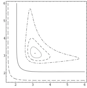
β→0,ΣR(L,β)diverges implying that we have ultraviolet as-ymptotic freedom for short distances and/or for high temper-atures, irrespective of the value ofλ. The overall behavior of the renormalized subdiagram can be acquainted from Fig. 1, where we draw contour plots ofΣR(L,β)/m, takingLandβin units ofm−1. The full line in Fig. 1 is the locus of the points such thatΣR(L,β) =0, which for largeL(β) approaches the straight lineβ=2.07m−1(L=2.07m−1);ΣR(L,β)is positive below this curve, negative above it, and reaches an absolute minimum,Σmin
R ≃ −0.0624m, at the pointL=β≃3.13m−1. This minimum (negative) value ofΣR(L,β)defines a “critical value” for λ,λmin=−(ΣminR )−1≃16.03m−1, for which the denominator of Eq. (12) vanishes and the effective coupling
constant diverges; forλ<λminthis never occurs. Also, if we takeLandβdifferent from 3.13m−1(but still in the region of negative values ofΣR), 0>ΣR(L,β)>ΣminR , the denominator of Eq. (12) vanishes for larger values ofλ(λ>λmin).
2 3 4 5 6
2 3 4 5 6
FIG. 1: Contour plots ofΣR(L,β)/m, withLandβin units ofm−1. The open dashed line corresponds toΣR(L,β)/m=0.2, the full line gives the points whereΣR=0, while the closed curves are for neg-ative values ofΣR/m,−0.053,−0.058 and−0.061 (dashed-dotted, dashed and dotted lines respectively). The dot is the location of the absolute minimum ofΣR.
The existence of a region in the parameter space (L,β) whereΣR is negative leads naturally to the onset of spatial confinement and thermal deconfinement, if the fixed coupling constant is high enough.
Consider initially the situation at T =0. In this case,
ΣR(L) has a zero at Lcmin≃2.07m−1, is negative for larger values of L, reaching a minimum (Σ(R0)min≃ −0.052m) at Lmaxc ≃2.82m−1. We present in Fig. 2ΣR(L)as a function of L. The existence of such a minimum implies that, for
λ≥λc =−(Σ( 0)min
R )−1≃19.16m−1, λ/g(L,λ) has a non-positive minimum value and vanishes for a lengthL(c0)(λ) be-longing to the interval¡Lminc ,Lmaxc ¤. This means that the sys-tem will be confined in a lengthL(c0)(λ), that is, starting with Lsmall (in the region of asymptotic freedom) the length can not go aboveL(c0)(λ)sinceg(L,λ)→∞asL→L(c0)(λ)[5].
In Fig. 3, we show the effective coupling constantg(L,λ)as a function ofL, for some values ofλ. We see clearly that, in the strong coupling regime, we have simultaneously asymp-totic freedom and spatial confinement, in the sense described above.
Let us now consider the effect of temperature, taking
2 3 4 5 6 L
-0.05 0.05 0.1 0.15 0.2 S
FIG. 2: Plot ofS=ΣR(L)/m, withLin units ofm−1.
1 2 3 4 5 6 L
5 10 15 20 25 30 g
FIG. 3: Plots of the effective coupling constantg(L,λ)as a function ofL(in units ofm−1), for some values ofλ(in units ofm−1): 5.0 (dashed line), 8.0 (dotted line), 11.0 (dotted-dashed line) and 19.16 (full line). The dotted vertical line, passing byLmax
c ≃2.82, is plotted as a visual guide.
L, is shown in Fig. 4 where we takeλ=25.0m−1and some values ofβ. Therefore, forβ<βd(λ),λ/g(L,β,λ)becomes positive for all values ofLand then the system is unconfined. Thus, Td(λ)corresponds to the deconfining temperature for the given fixed coupling constantλ≥λc.
Our finding that fermion spatial confinement exists in the strong coupling regime of the compactified Gross-Neveu model, being destroyed by raising the temperature, may ac-quire a physical meaning if we consider the Gross-Neveu model as an effective theory for the strong interaction between quarks. This corresponds to shrinking the gluon propagator similarly to the Fermi treatment of the weak force between leptons. In this sense, we will take the fermion mass as the constituent quark mass, m≈350MeV ≃1.75f m−1[17], in order to estimate the confining length and the deconfining temperature. We also take the fixed coupling constant with the minimum strength for confinement,λ=λc≃19.16m−1, corresponding to the maximum confining length at zero tem-perature,Lc≃2.82m−1. For this case, we findβd≃2.54m−1.
This choice leads toLc≃1.61f mandTd≃138MeV. These
2 3 4 5 6 L
-0.02 0.02 0.04 0.06 0.08 0.1 g-1
FIG. 4: Inverse of the effective coupling constantg−1(in units of λ−1), withλ=25.0m−1fixed, as a function ofL(in units ofm−1), for some values ofβ(in units ofm−1): 3.2, 2.356 and 2.2 (dashed, full and dotted lines respectively).
values are of the order of the experimentally measured pro-ton charge diameter (≈1.74f m) [18] and the estimated de-confining temperature (≈200MeV) for hadronic matter [19], respectively. It should be noticed that, despite of the crude-ness of this estimate, our result is in the range of the expected deconfining temperature of QCD.
In summary we have shown that, in the weak coupling sit-uation (λ<λc), the 3-D Gross-Neveu model presents only short-distance and high-temperature asymptotic freedom. For the strong coupling regime (λ>λc), we analytically demon-strate the simultaneous existence of asymptotic freedom and (for low enough temperatures) a singularity in the effective renormalized coupling constant at a lengthLc(λ), signalizing spatial confinement. This means that, if we start with a system of aquark-antiquark(understood as quanta of the fermionic Gross-Neveu model) pair bounded between two planes a dis-tanceL (<Lc(λ)) from one another (at some, low enough, temperature), it would not be possible to separate them a distance larger than Lc(λ). This spatial confinement of the quark-antiquarkpair could be interpreted as the existence of bound states (“baryon-like” states), characteristic of the model in the strong coupling regime. By raising the temperature, we find that the spatial confinement disappears at the deconfin-ing temperatureTd(λ). Notice that we refer to this property of the Gross-Neveu model asconfinement, understood in the sense described above,notof color confinement as it should happen for QCD. To account for color confinement we should consider a model that would accommodate gauge bosons, for instance Large-N QCD. This is the subject of a future investi-gation.
[1] D.J. Gross and A. Neveu, Phys. Rev. D10, 3235 (1974). [2] H. R. Christiansen, A. C. Petkou, M. B. Silva Neto, and N. D.
Vlachos, Phys. Rev. D62, 025018 (2000).
[3] J-P. Blaizot, R. M. Galain, and N. Wschebor, Ann. Phys.307, 209 (2003).
[4] L. Dolan and R. Jackiw, Phys. Rev. D9, 3320 (1974).
[5] A. P. C. Malbouisson, J. M. C. Malbouisson, A. E. Santana, and J. C. Silva, Phys. Lett. B583, 373 (2004).
[6] C. de Calan, P.A. Faria da Veiga, J. Magnen, and R. S´eneor, Phys. Rev. Lett.66, 3233 (1991).
[7] K. Gawedzki and A. Kupiainen, Phys. Rev. Lett. 55, 363 (1985); Nucl. Phys. B262, 33 (1985).
[8] W. Chen and M. Li, Phys. Rev. Lett.70, 884 (1993).
[9] V. S. Alves, M. Gomes, S. V. L. Pinheiro, and A. J. da Silva, Phys. Rev. D59, 045002 (1998).
[10] A. P. C. Malbouisson, J. M. C. Malbouisson, and A. E. Santana, Nucl. Phys. B631, 83 (2002).
[11] A. P. C. Malbouisson and J. M. C. Malbouisson, J. Phys. A: Math. Gen.35, 2263 (2002).
[12] L. M. Abreu, C. de Calan, A. P. C. Malbouisson, J. M. C. Mal-bouisson, and A. E. Santana, J. Math. Phys.46, 012304 (2005). [13] J. C. da Silva, F. C. Khanna, A. Matos Neto, and A. E. Santana,
Phys. Rev. A66, 052101 (2002).
[14] H. Queiroz, J. C. da Silva, F. C. Khanna, J. M. C. Malbouisson, M. Revzen, and A. E. Santana, Ann. Phys.317, 220 (2005). [15] A. Chodos, R. L. Jaffe, K. Johnson, C. B. Thorn, and V. F.
Weis-skopf, Phys. Rev. D9, 3471 (1974).
[16] C. A. Lutken and F. Ravndal, J. Phys. A: Math. Gen.21, L793 (1988).
[17] Particle Data Group, Phys. Lett. B592, 1 (2004); see page 475. [18] S. G. Karshenboim, Can. J. Phys.77, 241 (1999).