REMOVING THE INFLUENCE OF THE SERIAL CORRELATION ON THE MANN-KENDALL TEST
GABRIEL CONSTANTINO BLAIN
Instituto Agronômico de Campinas, Centro de Pesquisa e Desenvolvimento de Ecoisiologia e Biofísica,
Campinas, SP, Brazil
[email protected]
Received October 2012 - Accepted August 2013
ABSTRACT
The Whitening (PW), the Trend-Free Whitening (TFPW) and the Modiied Trend-Free Pre-Whitening (MTFPW) were developed to remove the inluence of serial correlations on the Mann-Kendall trend test. The main purpose of this study was to compare the performance of these algorithms for evaluating trends in auto-correlated series. The PW, TFPW and MTFPW were also applied to the monthly values of the rainfall (Pre), minimum (Tmin) and maximum (Tmax) air temperature data obtained from the weather station of Ribeirão Preto, State of São Paulo, Brazil. Sets of Monte Carlo simulations were carried out to evaluate the occurrence of the type I and the type II errors obtained from these three algorithms. The TFPW has the highest power. However, it also presented the highest occurrence of type I errors. The PW clearly limits the inluence of serial correlation on the occurrence of type I errors. Nevertheless, this feature is accomplished at a cost of a great reduction of its ability to detect trends. The MTFPW leads to a better balance between the probabilities of both statistical errors. It was also concluded that the hypothesis of the presence of no climate change in the location of Ribeirão Pareto cannot be accepted.
Keywords: Trends, climate change, auto-correlation.
RESUMO: REMOÇÃO DA INFLUÊNCIA DA CORRELAÇÃO SERIAL SOBRE O TESTE DE MANN-KENDALL
Os procedimentos denominados de Pre-Whitening (PW), Trend-Free Pre-Whitening (TFPW) e
Modiied Trend-Free Pre-Whitening (MTFPW) foram desenvolvidos para remover a inluência da correlação serial no teste de tendência de Mann-Kendall. O objetivo principal desse estudo foi comparar o desempenho desses três algoritmos para avaliar a presença de tendências em séries auto-correlacionadas. O PW, o TFPW e o MTFPW também foram aplicados nos dados mensais de precipitação pluvial e das temperaturas mínima e máxima do ar registrados em Ribeirão Preto, SP. Foram realizadas simulações de Monte Carlo para quantiicar a ocorrências dos erros tipo I e II associados à esses procedimentos. Embora o TFPW tenha apresentado o menor número de erros tipo II, o mesmo associou-se a maior frequência de ocorrência de erros tipo I. O PW limitou a inluência da correlação serial sobre a ocorrência do erro tipo I. Entretanto, essa última característica é atingida ao custo de uma importante redução em sua habilidade de detectar reais tendências. O MTFPW leva a um melhor equilíbrio entre as probabilidades de ocorrência desses dois erros estatísticos. Concluí-se também que a hipóteConcluí-se da ausência de tendências climáticas na localidade de Ribeirão Preto não pode ser aceita.
1. INTRODUCTION
The current concern and uncertainties associated with the global warming have motivated several authors to investigate the presence of climate trends, at regional scale, in several parts of the world. According to Önöz and Bayazit (2011) ‘climate change has given an impetus to trend detection studies of hydro-meteorological variables’. Naturally, this impetus can also be seen in studies related to agro-meteorological variables. According to Wilks (2011), investigating possible trend of the central tendency of a dataset is of interest in the context of climate changes.
The Mann-Kendall test (MK; Mann, 1945; Kendall and Stuart, 1967) is perhaps the most used mathematical method for detecting trends in time series. Considering only the period between 2002 and 2012, authors such as Yue et al. (2002), Burn and Elnur, 2002, Adamowski and Bougadis (2003), Yue et al. (2003), Yue and Hashino (2003), Burn et al. (2004), Yue and Pilon (2004), Sansigolo (2008), Sansigolo and Kayano (2010), Tabari and Talaee (2011), Blain (2011a,b,c), Minuzzi et al. (2011), Blain and Pires (2011), Streck et al. (2011), Back et al. (2012) and Blain (2012a,b) used this test to evaluate signals of climate change in several parts of the Globe. As a consequence of this widespread use, several scientiic studies have addressed the strengths and the limitations of this statistical test (Blain, 2013). The strengths of the MK are usually associated with its simple concept and with the fact that as a nonparametric procedure that does not assume a speciic joint distribution of the data, it is minimally affected by departures from normality (Yue and Pilon, 2004).
The limitations of this trend test are associated with the fact that it was originally designated for uncorrelated data. Thus, the null hypothesis (H0) of the MK test assumes that the data are realized values of independent and identically distributed (iid) variables (Chandlerand Scott, 2011). Therefore, from a strictly statistical point of view, the non-acceptance of such a H0 only implies that the sample data does not meet this iid assumption. However, as described in several studies such as Blain (2013) the rejection of such a H0 is often taken as an evidence of the presence of trend in a given meteorological time series. Therefore, given that environmental variables, such as meteorological, agrometeorological and hydrological data, frequently exhibit same form of positive auto-correlation (Yue et al. 2002, Fleming and Clark, 2002, Burn and Elnur, 2002, Burn et al, 2008, Khaliq et al., 2009 and Blain, 2012b), a signiicant MK outcome may be erroneously interpreted as a signal of climate change even though no (true) trend is present (Von Storch and Navarra, 1995). Further information regarding the deinition of serial correlation can be found in Wilks (2011).
As can be noted from the MK literature (Von Storch and Navarra, 1995, Yue et al. 2002 and Flemingand Clark, 2002, among many others) the rejection of the aforementioned Ho in the presence of no trend is regarded as a false rejection. Thus, we may indicate that the presence of a signiicant positive serial correlation increases the occurrence of type I errors, making it greater than the (adopted) nominal signiicance level (Von Storch and Navarra, 1995, Yue et al. 2002, Fleming and Clark, 2002, Yue et al., 2003, Yue and Hashino, 2003, Burn et al., 2004, Yue and Pilon, 2004, Önöz and Bayazit, 2011 and Blain 2013). Several efforts have been carried out to avoid these false trend detections. Generally speaking, these efforts can be classiied into two different approaches (Hamed, 2009). The irst one modiies the MK calculation algorithm to account for the presence serial correlation. Further information regarding this irst approach, including the advantages of its use, can be found in Hamed and Rao (1998), Yue et al. (2002), Yue and Wang (2004) and Khaliq et al. (2009), among others. The second approach manipulates the original data to meet the assumption of no temporal dependence (Hamed, 2009). The natural advantage of this latter approach over the irst one is that it can be applied to other trend tests besides the MK (Khaliq et al., 2009). This second approach is often carried out by adopting either the procedure called pre-whitening (PW; Kulkarni and Von Storch, 1995, and Von Storch and Navarra, 1995) or the procedure called trend-free pre-whitening (TFPW; Yue et al., 2002). Each one of these procedures (or algorithms) has its own advantages and drawbacks.
The advantage of the PW is that it reduces the occurrence of the type I errors close to the adopted (nominal) signiicance level (Yue et al., 2002, Bayazit and Önöz, 2007 and Blain, 2013, among many others). However, this procedure may also lead to a loss of power, ‘so that a signiicant trend may escape
probability of rejecting a false H0. This modiied version is referred to as MTFPW.
Despite all these efforts to ensure that the null hypothesis of no trend will be correctly rejected/accepted, authors such as Khaliq et al. (2009) and Sansigolo and Kayano (2010) indicate that the majority of the studies that investigates trends in time series assume that the data are serially independent. In addition, according to Blain (2013) the inluence of serial correlations on trend analyses is frequently neglected in Brazilian agrometeorological studies. All these statements, associated with the assumption that ‘chasing greenhouse signature involves searching for traces of changes in a time series of variables of concern’ (Radziejewski and Kundzewicz, 2004), reinforce the need to evaluate the occurrence oftype I and II errors obtained from the PW, TFPW and MTFPW algorithms. Thus, the main aims of this study were (i) to evaluate the power of these algorithms when they are applied to auto-correlated series that comprise a (true) trend component and, (ii) to compare the performance of the PW, TFPW and MTFPW, when these three statistical algorithms are applied to trend-free datasets with different levels of serial correlation. Finally, as a case of study these three algorithms were also applied to the monthly values of the rainfall (Pre), minimum (Tmin) and maximum (Tmax) air temperature data obtained from the weather station of Ribeirão Preto, State of São Paulo, Brazil. We expect that this study should provide evidences that help to improve the interpretation of the different outcomes obtained from the aforementioned algorithms by highlighting their strengths and drawbacks. We also expect that this study should provide evidences for accepting/rejecting the hypothesis of the presence of climate change signals in one of the most important agricultural region of the State of São Paulo, Brazil (RibeirãoPreto).
2. DATA AND METHODS
The monthly air temperature data were obtained from the weather station of RibeirãoPreto (Agronomic Institute; IAC/APTA/SAA-SP; 21º11’S; 47º48’W; 621m). The length of records is 69 years (1943-2011). These series do not have missing data and their consistencies have been previously assessed in Blain (2011a,b). All hypothesis tests were performed at the 5% signiicance level.
Given a dataset X consisting of x values with sample size SS, the MK calculation starts by estimating the S statistic.
As indicated in Mann (1945) and Kendall; Stuart (1967) when SS≥8 the distribution of S approaches the Gaussian form with mean E(S)=0 and variance V(S) given by:
where ti is the number of ties of length m.
The statistic S is then standardized (Equation 3) resulting in the MK inal value. The signiicance of the MK statistic can be estimated from the normal cumulative distribution function. Positive (negative) MK values indicate the presence of increasing (decreasing) trends.
The initial step of the three algorithms (PW, TFPW and MTFPW) is to estimate the lag-1 auto-correlation coeficient from the original time series (r-original). If r-original is not signiicant the original MK test is applied to the original series and no other step needs to be carried out. The second step of the PW is to remove the (signiicant) r-original from the original series. Equations 1, 2 and 3 are then applied to this pre-whitened series. The second step of the TFPW algorithm is to estimate and remove the slope of the trend from the original series (step 2; Equation 4). The lag-1 auto-correlation coeficient is then estimated from this detrended series (r-detrended; step 3). If r-detrended is found to be signiicant, it is removed from this detrended series (step 4). The TSA (Equation 4) is then superimposed onto this last series (referred to as blended series; step 5). According to Yue et al. (2002), this blended series preserves an existing trend but is no longer inluenced by the presence of signiicant serial correlations. Equations 1, 2 and 3 are then applied to this blended series. Further information regarding the TFPW algorithm can be found in Yue et al. (2002). As described in Önöz and Bayazit (2011), the steps 2 and 3 of the MTFPW are the same of the TFPW. However, its fourth step is to remove the r-detrended from the original time series. The MK test is then applied to this modiied-original series.
Equation 4 is frequently referred to as the Theil-Sen Approach (TSA; Sen, 1968) and, it is often used to estimate the slope of an existing trend. According to Yue et al. (2002) the time series should not be detrended if its TSA value is ‘almost equal to zero’ (Yue et al., 2002). In this study, a non signiicant TSA value was considered as being almost equal to zero. The signiicance of each TSA value was evaluated by using the bootstrap approach described in Yue and Pilon (2004). The number of bootstrapped samples required for constructing the related null distributions was set equal to 5000. The signiicance
(
)
∑ ∑
− = =+ − = 1 1 1 sgn SS i SS i j j xi x S (1) < → + = → > → − = 0 ) ( 1 0 0 0 ) ( 1 S s V S S S s V S MK (3) − = b -a x xMedian a b
TSA ∀ b < a
(4) ( )( ) ( )( ) 18 5 2 1 5 2 1 )
( = − + −
∑
=1 − +SS
m tim m m
of the auto-correlation coeficients were evaluated as described in Wilks (2011).
The Monte Carlo simulations were based on Equation 5.
E(X), r and T are, respectively, the mean, the lag 1 auto-correlation coeficient and the trend component of the generating process; ξt is a white noise process with zero mean and variance equal to √[Var(X)*(1-r2)]; t represents the time unit which varies from 1 to N. N is the sample size which was set equal to 30, 60, and 90. These sample sizes represent series that comprise 1, 2 and 3 climatological normal periods. By following Önöz and Bayazit (2011), the values of r were set =0.0 (an uncorrelated process), =0.2, =0.4 and =0.6. By following Yue et al. (2002), the mean and the coeficient of variation of the generating process were, respectively, set equal to 1 and 0.50.
2.1 The type II error
T was set equal to 0.002, 0.004, 0.006 and 0.008. From these adopted values the mean of the simulated process increases by 2, 4, 6 and 8% per 10 time units. At this point, it is worth mentioning that the Monte Carlo experiments carried out in this study can be regarded as pure mathematical evaluations. However, these simulations were carried out concerning meteorological as well as agrometeorological time series. Thus, we assumed that values of T that could lead to a magnitude of change greater than 80%, per 100 time units, would product unrealistic results. The Monte Carlo simulations generated Ns=10000 time series for each r, N and T value. The PW, TFPW and MTFPW, performed at the 5% signiicance level, were applied to each one of these series. By denoting the probability of occurrence of a type II error as β, the quantity 1- β is frequently referred to as “the power of the test”. Given that all simulated series have a true trend, the power of the tests, for each r, N and T value, is simple the ratio between the number of simulations in which the null hypothesis of no trend was (correctly) rejected (Nrej) and Ns. Only increasing trends were evaluated since the power of the tests is identical for both upward and downward trends (Yue et al., 2002 and Yue and Pilon, 2004).
2.2 The type I error
The Monte Carlo simulations generated Ns=10000 time series for each r and N value. Naturally, T was set equal to zero. The PW, TFPW and MTFPW, performed at the 5% signiicance level, were applied to each one of the trend-free simulated series. From statistical theory and given that equation 5 has, in this case, no trend component, we should expect (approximately)
500 false rejections of H0. In other words, it is expected that the rejection rate obtained from this large number of trend-free datasets (10000) should be close to the nominal signiicance level (5%; 500/10000) adopted in the present study. Otherwise, the effect of serial correlation on the occurrence of type I errors is not being effectively removed.
3. RESULTS AND DISCUSSION
As can be noted from several studies such as Yue et al. (2002), Fleming and Clark (2002), Yue and Pilon (2004), Yue and Wang (2004), Önöz and Bayazit (2011) and Blain (2013), the power of any trend test is an increasing function of the sample size and of the slope of the trend. The results depicted in Figure 1 are consistent with this last statement. As can be noted, the highest rejection rates are observed for the highest values of N and T (Figure 1). The low rejection rates observed for the smallest values of T and N are also consistent with the results found by Radziejewski and Kundzewicz (2004). After having evaluated the power of 5 trend tests (including the MK), Radziejewski and Kundzewicz (2004) stated that trend tests may not be able to detect either weak changes or changes which have not lasted long.
By considering only the uncorrelated series (r=0), one may verify that the power of the three algorithms are similar to each other. However, as the serial correlation increases, the difference among the rejection rates, obtained from each approach, also increases (Figure 1). This last consideration agrees with the results observed in the study of Khaliq et al. (2009). By following these authors, we may indicate that the outcomes of the PW and the TFPW are likely to differ from each other particular for signiicantly auto-correlated data. As can be noted from Figure 1, the higher the auto-correlation, the greater is the difference among the power of the algorithms.
According to Önöz and Bayazit (2011) the estimated slope of the trend (TSA in the present study) tends to be larger than its true slope (Strue) due to the interaction between trend and serial correlation. After evaluating the TFPW algorithm, described in the previous section, one may argue that if TSA is greater than Strue, the obtained detrended series will have an auto-correlation coeficient lower than the (true) auto-correlation of the process (Önöz and Bayazit, 2011). Therefore, for such cases, the TFPW may not totally remove the inluence of serial correlation on the trend analysis. This last inference seems to be consistent with the results obtained from the lowest values of N and T (Figure1a-i). For such cases, the power of the TFPW can be seen as an increasing function of the auto-correlation coeficient. According to Bayazit and Önöz (2007) along with its inluence on the type I errors, the presence of positive serial correlations also decreases the frequency of occurrence of the xt=E(X) + r(xt-1 – E(X)) + ξt + T
type II errors. Naturally, this causes no problem (Bayazit and Önöz, 2007). On the other hand, for the highest values of N and T (Figure 1h-l) the rejection rates obtained from the TFPW (r≥0.2) were similar to those obtained from the uncorrelated series. A possible reason for this last feature may be the fact that as the sample size and the slope of the trend increase the TSA approaches the true slope of the real trend.
As can be easily noted from Figure 1 (r≥0.2), the lowest rejection rates were obtained by applying the PW. In addition, after Bayazit and Önöz (2007) we may state that the PW leads to a real loss of power given that the frequencies of occurrence of type II errors increase as the serial correlation increases. From the results depicted in Figure 1, one may indicate that the power of the PW tends to be a decreasing function of the auto-correlation coeficient. By following authors such as Yue et al. (2002), Fleming and Clark (2002), Khaliq et al. (2009) and Bayazit and Önöz (2007) we may indicate that the use of the PW approach should be avoided given that it underestimate the magnitude of the trend and its statistical signiicance.
Moreover, according to Khaliq et al. (2009) the PW tends to be more conservative than the TFPW in identifying stations with signiicant trends. Therefore, there is a possibility that stations with weak temporal signals would be overlooked by the PW (Khaliq et al., 2009). These last statements are also in agreement with the results depicted in Figure 1.
The MTFPW was proposed by Bayazit and Önöz (2007) to correct for the ‘inlation’ of the trend caused by the TFPW calculation algorithm. Thus, one may expect that the power of the MTFPW should belower than the power of the TFPW. This last inference is supported by the results depicted in Figure 1. As can be noted, when r was set equal to or greater than 0.2, the rejection rates obtained from the TFPW was always greater than those obtained from the MTFPW. Regarding the PW approach, it is also evident that the MTFPW tends to outperform the PW as r increases. Finally, the results depicted in Figure 1 clearly indicate that the TFPW is the most powerful test.
Based only on the results depicted in Figure 1, one may argue that the TFPW is the most appropriate method
0.0 0.1 0.2 0.3 0.4 0.5 0.6 0.7 0.8 0.9 1.0 H o: R at e o f r ej ect io
n (a) N=30
T=0.002 PW TFPW MTFPW (e) N=60 T=0.002 (i) N=90 T=0.002 0.0 0.1 0.2 0.3 0.4 0.5 0.6 0.7 0.8 0.9 1.0
0.0 0.2 0.4 0.6
H o: R at e o f r ej ec tio n
Coefficient of auto-correlation
(d) N=30 T=0.008 PW
TFPW MTFPW
0.0 0.2 0.4 0.6
Coefficient of auto-correlation
(h) N=60 T=0.008
0.0 0.2 0.4 0.6
Coefficient of auto-correlation
(l) N=90 T=0.008 0.0 0.1 0.2 0.3 0.4 0.5 0.6 0.7 0.8 0.9 1.0 H o: R at e o f r ej ect io
n (b) N=30
T=0.004 PW TFPW MTFPW (f) N=60 T=0.004 (j) N=90 T=0.004 0.0 0.1 0.2 0.3 0.4 0.5 0.6 0.7 0.8 0.9 1.0 H o: R at e o f r ej ec tio
n (c) N=30
T=0.006 PW TFPW MTFPW (g) N=60 T=0.006 (k) N=90 T=0.006
Figure 1 - Rejection rates of 10000 simulated series obtained from three different approaches to calculating the Mann-Kendall test (at the 5%
for detecting trends in auto-correlated series because it has presented the lowest frequency of occurrence of type II errors for all N and T values. However, it has to be emphasized that the aforementioned analyses did not address the probability of rejecting a true Ho. Given that authors such as Hamed (2009) state that ‘knowing the correct frequency of occurrence of a type I error is of primary concern’, the probability of the PW, TFPW and MTFPW to falsely reject a (true) Ho has to be known. According to Blain (2013) the TFPW effectively limit the inluence of the serial correlation on the occurrence of type I errors. This statement is not consistent with the results depicted in Figure 2. As can be noted, the rejection rates obtained from the (trend-free) auto-correlated series by applying the TFPW are signiicantly greater than the 5% adopted signiicance level. For instance, the rejection rate obtained from the TFPW by setting N=90 and r=0.4 is 0.23 (almost ive times greater than the 0.05 critical level). Moreover, the (false) rejection rates obtained from this algorithm seems to be an increasing function of the serial correlation. In other words, the results found in this study are in agreement with Khaliq et al. (2009) and Bayazit and Önöz (2007) in the sense that the TFPW may not be capable of preserving the nominal signiicance level. Moreover, the results depicted in Figure 2 do not allow us to agree with the statement of Blain (2013) that the TFPW is as good as the PW in not rejecting a true H0 (Figure 2). Also regarding the probability of falsely rejecting a H0, the performance of both PW and MTFPW improves as the sample size increases. As can also be noted from Figure 2, as the sample size increases, the performance of the MTFPW tends to be as good as the performance of the PW in not rejecting a true H0. Finally, for the serially independent series (r=0; Figure2) the frequency of occurrence of the type I errors, obtained from the three algorithms, were virtually equal to the adopted 5% signiicance level.
By comparing the results depicted in Figures 1 and 2, it becomes clear that there is a trade-off between the frequency of occurrence of the type I errors and the power of the three algorithms. From the results depicted in Figure 1 we may indicate that the TFPW has the highest power. However, this
desirable feature is achieved at a cost of detecting false trends too often (Bayazit and Önöz, 2007). On the other hand, the PW approach clearly limits the inluence of serial correlation on the MK outcomes by reducing the occurrence oftype I errors close to the adopted signiicance level. Nevertheless, this last desirable feature is accomplished at a cost of a great reduction of its ability to detect true trends. As can also be noted from Figures 1 and 2, the performance of both PW and MTFPW improves as the sample size increases. In general, for these two algorithms, the frequency of occurrence of both type I and type II errors tends to decreases as N increases. A similar conclusion cannot be drawn from the results obtained by applying the TFPW (Figure 1). The frequency of occurrence of type I errors obtained by applying this last approach was not affected by the different values of N. Finally, it is worth mentioning that the Monte Carlo experiments were carried out considering solely a particular case of monotonic trends: the linear shape. Although the study of Yue and Pilon (2004) has provided empirical evidence indicating that the MK test is only slightly inluenced by the shape of the trends, we may indicate that further studies are still required to assess the performance of the three aforementioned algorithms under nonlinear trend conditions. However, in the following section, no assumption was made about the shape of the trends.
3.1 Case study
The results and discussions described in the previous section were used to help the interpretation of the outcomespresented in Tables 1 and 2. As can be noted from studies carried out in several regions of South America (Vincent et al., 2005 and Sansilogo and Kayano, 2010) the minimum air temperature is a meteorological variable that often shows signiicant signals of climate trends. After Sansigolo and Kayano (2010) have evaluated long-term variations of seasonal and annual indices obtained from Tmin, Tmax and Pre series of the State of Rio Grande do Sul, Brazil, they indicated that the annual and seasonal Tmin indices have shown signiicant warming trends. Regarding the Tmax records, these authors indicated
0.0 0.1 0.2 0.3 0.4 0.5 0.6 0.7 0.8 0.9 1.0
0.0 0.2 0.4 0.6
H
o:
R
at
e o
f r
ej
ect
io
n
Coefficient of auto-correlation (a) N=30
PW
TFPW
MTFPW
0.0 0.2 0.4 0.6
Coefficient of auto-correlation (b) N=60
0.0Coefficient of auto-correlation0.2 0.4 0.6 (c) N=90
Figure 2 - Rejection rates of 10000 trend-free simulated series obtained from three different approaches of calculating the Mann-Kendall. The
that the only signiicant trend was found for the summer series. This last result is associated with a cooling trend. Regarding the precipitation records, the only signiicant increasing trend was also found for the summer series (Sansilogo and Kayano, 2010). By following Vincent et al. (2005) we may indicate that the air temperature are changing in South America because signiicant warning trends were observed in indices based on daily minimum air temperatures. However, Vincent et al. (2005) also indicated the presence of no consistent change in the indices derived from the daily maximum air temperatures. Dufek and Ambrizzi (2007) analyzed indices derived from daily rainfall data obtained from 59 locations of the State of São Paulo (1950-1999). According to these authors, 59.3% (8.5%) of the analyzed Pre series have shown signiicant increasing (decreasing) trends in the annual amounts.
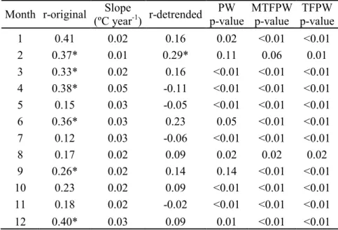
As can be observed from Table 1, for those months in which the estimated auto-correlation coeficient, obtained from the detrended series (r-detrended; step 3 of the TFPW and MTFPW algorithms) is not signiicant, the outcomes of the TFPW and MTFPW are equal to each other. For such cases, the blended series and the modiied-original seriesare equal to the original series. As expected, for the cases in which the estimated auto-correlation coeficient, obtained from the original series (r-original) is not signiicant, i.e. r≈0, the p-values associated with the PW, TFPW and MTFPW are equal to each other. This last result agrees with those depicted in Figure 1 and 2 by setting r equal to zero.
Finally, one may argue that the most important difference among the three algorithms is observed when both r-original
and r-detrended are signiicant (Months of February). For such case, the p-value associated with the PW, TFPW and MTFPW were equal to 0.11, 0.06 and 0.01, respectively. From the results depicted in Figure 2b, we may infer that the false rejection rates obtained from the PW and MTFPW for series with a sample size 60<N<90 and with a true auto-correlation coeficient between 0.37 (r-original) and 0.29 (r-detrended) are close to each other. Moreover, for such values of r and N the results depicted in Figure 1 allow us to infer that the MTFPW is slightly more powerful than the PW. By considering that for approximately equal rates of false rejections, the test with highest power should be preferred (Önöz and Bayazit, 2011) the aforementioned trend (detected during the Months of February) was regarded as having a p-value equal to 6%.
In spite of the difference among the p-values obtained from the three algorithms, the results depicted in Table 1 indicate the presence of important traces of changes in the Tmin series of RibeirãoPreto. It is worth emphasizing that even the less powerful test (PW) has indicated the presence of signiicant increasing trends (at the 5% signiicance level) in ten months. By considering the same signiicance level, the MTFPW has indicated the presence of signiicant increasing trends in 11 months. Thus, the results shown in Table 1 and the analysis of the performance of the three trend-detection algorithms (Figures 1 and 2) do not allow us to accept the hypothesis of no sign of trend in Tmin series of the location of Ribeirão Preto.
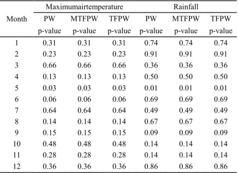
Before analyzing the outcomes presented in Table 2, it has to be emphasized that the auto-correlation function indicated the presence of no signiicant serial correlation in the Tmax
Month r-original Slope
(ºC year-1
) r-detrended
PW p-value
MTFPW p-value
TFPW p-value
1 0.41 0.02 0.16 0.02 <0.01 <0.01
2 0.37* 0.01 0.29* 0.11 0.06 0.01
3 0.33* 0.02 0.16 <0.01 <0.01 <0.01
4 0.38* 0.05 -0.11 <0.01 <0.01 <0.01
5 0.15 0.03 -0.05 <0.01 <0.01 <0.01
6 0.36* 0.03 0.23 0.05 <0.01 <0.01
7 0.12 0.03 -0.06 <0.01 <0.01 <0.01
8 0.17 0.02 0.09 0.02 0.02 0.02
9 0.26* 0.02 0.14 0.14 <0.01 <0.01
10 0.23 0.02 0.09 <0.01 <0.01 <0.01 11 0.18 0.02 -0.02 <0.01 <0.01 <0.01
12 0.40* 0.03 0.09 0.01 <0.01 <0.01
Table 1 - Three different approaches to calculating the Mann-Kendall test (PW, TFPW and MTFPW) applied to minimum air temperature records.
and Pre series. Thus, the outcomes obtained from the three algorithms were equal to each other.
Regarding the Tmax series the results presented in Table 2 are similar to those found by Sansigolo and Kayano (2010) in the sense that the only signiicant outcome is associated with a decreasing trend. However, for this weather station of the State of São Paulo this change has occurred during the last month of the fall season (May; TSATmax=0.01°C yr-1). It is worth emphasizing that also during the mouths of May it is observed the only signiicant increasing trend in the rainfall series (TSAPre=0.54 mm yr-1).
4. FINAL REMARKS
This study has addressed the advantages and drawbacks of three algorithms (PW, TFPW and MTFPW) developed to remove the inluence of serial correlation on the MK test. The results obtained from Monte Carlo simulations and from a case of study (weather station of Ribeirão Preto) clearly indicate that the TFPW is the most powerful test. However, the Monte Carlo simulations indicate that this desirable feature is associated with a high probability of falsely reject a (true) H0 of no trend. On the other hand, it was observed that the PW has the lowest probability of rejecting a true Ho. However, this desirable feature is associated with a great reduction of its power.
The Monte Carlo simulations also indicate that the MTFPW is almost as good as the PW in preserving the nominal
Month
Maximumairtemperature Rainfall
PW MTFPW TFPW PW MTFPW TFPW
p-value p-value p-value p-value p-value p-value
1 0.31 0.31 0.31 0.74 0.74 0.74 2 0.23 0.23 0.23 0.91 0.91 0.91 3 0.66 0.66 0.66 0.36 0.36 0.36 4 0.13 0.13 0.13 0.50 0.50 0.50 5 0.03 0.03 0.03 0.01 0.01 0.01 6 0.06 0.06 0.06 0.69 0.69 0.69 7 0.64 0.64 0.64 0.49 0.49 0.49 8 0.14 0.14 0.14 0.67 0.67 0.67 9 0.15 0.15 0.15 0.09 0.09 0.09 10 0.48 0.48 0.48 0.14 0.14 0.14 11 0.28 0.28 0.28 0.14 0.14 0.14 12 0.36 0.36 0.36 0.86 0.86 0.86
Table 2 - Three different approaches to calculating the Mann-Kendall test (PW, TFPW and MTFPW) applied to maximum air temperature and
rainfall records. The slopes of the trends and the Lag-1 auto-correlation coeficient (r-original) are also shown. Weather station of RibeirãoPreto (1943-2011), State of São Paulo, Brazil.
signiicance level. As the sample size increase, the occurrences of type I errors obtained from this two algorithms become close to each other. It was also observed that the MTFPW tends to be more powerful than the PW. Thus, the use of the MTFPW leads to a better balance between the probabilities of the type I and the type II errors.
The results of the Monte Carlo experiments were also used to improve our interpretation of the outcomes obtained by applying these three algorithms to the monthly values of the Tmin, Tmax and Pre data of the weather station of Ribeirão Preto (State of São Paulo, Brazil). This analysis revealed the presence of important traces of changes in the Tmin series.Regarding the Tmax and Pre series, the only signiicant outcomes were found during the months of May. For the Tmax and Pre series it was observed decreasing and increasing trends, respectively.
5. REFERENCES
ADAMOWSKI, K.; BOUGADIS, J. Detection of trends in annual extreme rainfall. Hydrological Process, v. 17, n. 1, p. 3547-3560, 2003.
BACK, A. J.; BRUNA, E. D.; VIEIRA, H. J. Tendências climáticas e produção de uva na região dos Vales da Uva Goethe. Pesquisa Agropecuária Brasileira, v. 47, n. 4, p. 497-504, 2012.
BLAIN, G. C. Aplicação do conceito do índice padronizado de precipitação à série decendial da diferença entre precipitação pluvial e evapotranspiração potencial. Bragantia, v. 70, n. 1, p. 234-245, 2011a.
BLAIN, G. C. Cento e vinte anos de totais extremos de precipitação pluvial máxima diária em Campinas, Estado de São Paulo: análises estatísticas. Bragantia, v. 70, n. 3, p. 722-728, 2011c.
BLAIN, G. C. Considerações estatísticas relativas a seis séries mensais de temperatura do ar da secretaria de agricultura e abastecimento do Estado de São Paulo. Revista Brasileira de Meteorologia, v. 26, n. 2, p. 279-296, 2011b.
BLAIN, G. C. Monthly values of the standardized precipitation index in the State of São Paulo, Brazil: trends and spectral features under the normality assumption. Bragantia, v. 71, n. 1, p. 122-131, 2012a.
BLAIN, G. C.; PIRES, R.C.M. Variabilidade temporal da evapotranspiração real e da razão entre evapotranspiração real e potencial em Campinas, Estado de São Paulo. Bragantia, v. 70, n. 2, p. 460-470, 2011.
BLAIN, G.C. Revisiting the probabilistic definition of drought: strengths, limitations and an agrometeorological adaptation, Bragantia, Campinas, v.71, n.1, p.132-141, 2012b.
BLAIN, G. C. The Mann-Kendall test: the need to consider the interaction between serial correlation and trend. Acta Scientiarum. Agronomy, v. 35, n. 4, p. 557-564, 2013. BURN, D. H.; CUNDERLIK, J.; PIETRONIRO, A. Climatic
inluences on streamlow timing in the headwaters of the Mackenzie River Basin. Journal of Hydrology, v. 352, n. 1, p. 225-238, 2008.
BURN, D. H.; CUNDERLIK, J.; PIETRONIRO, A.Hydrological trends and variability in the Liard River basin. Hydrological Sciences Journal, v. 49, n. 1, p. 53-67, 2004.
BURN, D. H.; ELNUR, A. H. Detection of hidrological trends and variability. Journal of Hydrology, v. 255, n. 1, p. 107-122, 2002.
CHANDLER, R. E.; SCOTT, M. E. Statistical methods for trend detection and analysis in the environmental analysis. 1st ed. Chichester: John Wiley & Sons, 2011. DUFEK, A.S.; AMBRIZZI, T. Precipitation variability in Sao
Paulo State, Brazil, Theoretical and Applied Climatology, v. 93, p. 167-178, 2007.
FLEMING, S. W.; CLARKE, G. K.C. Autoregressive Noise, Deserialization, and Trend Detection and Quantiication in Annual River Discharge Time Series. Canadian Water Resources Journal, v. 27, n. 3, p. 335-354, 2002.
HAMED, K. H. Exact distribution of the Mann–Kendall trend test statistic for persistent data. Journal of Hydrology, v. 365, n. 1, p. 86-94, 2009.
HAMED, K. H.; RAO, R. A modiied Mann-Kendall trend test for auto-correlated data. Journal of Hydrology, v. 204, n. 1, p. 182-196, 1998.
KENDALL, M. A.; STUART, A. The advanced theory of statistics. 2nd ed. Londres: Charles Grifin, 1967.
KHALIQ, M.N.; OUARDA, T. B. M. J.; GACHON, P.; SUSHAMA, L.; ST-HILAIRE, A. Identification of hydrological trends in the presence of serial and cross correlations: A review of selected methods and their application to annual low regimes of Canadian rivers. Journal of Hydrology, v. 368, n. 1, p. 117-130, 2009. KULKARNI, A., VON STORCH, H., Monte Carlo experiments
on the effect of serial correlation on the Mann–Kendall test of trend. Meteorologische Zeitschrift, v.4, n.2, p.82–85, 1995
MANN, H.B. Non-parametric tests against trend. Econometrica, v. 13, n. 3, p.245-259, 1945.
MINUZZI, R. B.; CARAMORI, P. H.; BORROZINO, E. Tendências na variabilidade climática sazonal e anual das temperaturas máxima e mínima do ar no Estado do Paraná. Bragantia, v. 70, n. 2, p. 471-479, 2011.
ÖNÖZ, B.; BAYAZIT, M. Block bootstrap for Mann–Kendall trend test of serially dependent data. Hydrological Process, v. 26, n. 15, p. 1–19, 2011.
RADZIEJEWSKI, M.; KUNDZEWICZ, Z. W. Detectability of changes in hydrological records. Hydrological Sciences Journal, v.49, n.1 p.39-51, 2004
SANSIGOLO, C. A. Distribuições de extremos de precipitação diária, temperatura máxima e mínima e velocidade do vento em Piracicaba, SP (1917-2006). Revista Brasileira de Meteorologia, v. 23, n. 3, p. 341-346, 2008.
SANSIGOLO, C. A.; KAYANO, M. T. Trends of seasonal maximum and minimum temperatures and precipitation in Southern Brazil for the 1913–2006 period. Theoretical and Applied Climatology, v. 101, n. 101, p. 209–216, 2010. SEN, P. K.; Estimates of the regression coefficient based
on Kendall’s tau. Journal of the American Statistical Association, v. 63, n. 1, p. 1379–1389, 1968.
STRECK, N. A.; GABRIEL, L. F.; HELDWEIN, A. B.; BURIOL, G. A.; DE PAULA, M. G. Temperatura mínima de relva em Santa Maria, RS: climatologia, variabilidade interanual e tendência histórica. Bragantia, v. 70, n. 3, p. 696-706, 2011.
TABARI, H.; TALAEE, P. H. Recent trends of mean maximum and minimum air temperatures in the western half of Iran. Meteorology and Atmospheric Physics, v. 11, n. 3-4, p. 121-131, 2011.
M.A.; GRIMM, A.M.; MARENGO, J.A.; MOLION. L.; MONCUNILL, D.F.; REBELLO, E.; ANUNCIAÇÃO, Y.M.T.; QUINTANA, J.; SANTOS, J.L.; BAEZ, J.; CORONEL, G.; GARCIA, J.; TREBEJO, I.; BIDEGAIN, M.; HAYLOCK, M.R.; KAROLY, D. Observed trends in indices of daily temperature extremes in South America 1960-2000. Journal of Climate, Washington, v.18, p.5011-5023, 2005.
VON STORCH, H.; NAVARRA, A. Analysis of Climate Variability: Applications of Statistical Techniques. Berlin: Springer, 1995.
WILKS, D. S. Statistical methods in the atmospheric sciences. 3rd ed. San Diego: Academic Press, 2011. YUE, S., HASHINO, M. Temperature trends in Japan: 1900–
1996. Theoretical and Applied Climatology, v. 75, n. 1, p. 15–27, 2003.
YUE, S., PILON, P. A comparison of the power of the t test, Mann-Kendall and bootstrap tests for trend detection. Hydrological Sciences Journal, v. 49, n. 49, p. 53-37, 2004. YUE, S., PILON, P., PHINNEY, B. Canadian streamflow
trend detection: impacts of serial and cross-correlation. Hydrological Sciences Journal, v. 48, n. 1, p. 51–64, 2003. YUE, S.; PILON, P. J.; PHINNEY, B.; CAVADIAS, G. The
inluence of autocorrelation on the ability to detect trend in hydrological series. Hydrological Process, v. 16, n. 16, p. 1807–1829, 2002.