Motion in Environments Varying in Space and Time
Lili Jiang1,3, Qi Ouyang1,2, Yuhai Tu1,3*
1Center for Theoretical Biology and School of Physics, Peking University, Beijing, China,2The State Key Laboratory for Artificial Microstructures and Mesoscopic Physics, School of Physics, Peking University, Beijing, China,3IBM T. J. Watson Research Center, Yorktown Heights, New York, United States of America
Abstract
Escherichia colichemotactic motion in spatiotemporally varying environments is studied by using a computational model based on a coarse-grained description of the intracellular signaling pathway dynamics. We find that the cell’s chemotaxis drift velocityvdis a constant in an exponential attractant concentration gradient [L]/exp(Gx).vddepends linearly on the exponential gradientGbefore it saturates whenGis larger than a critical valueGC. We find thatGCis determined by the intracellular adaptation ratekRwith a simple scaling law:GC!k1=2
R . The linear dependence ofvdonG=d(ln[L])/dxdirectly demonstrates E. coli’s ability in sensing the derivative of the logarithmic attractant concentration. The existence of the limiting gradient GCand its scaling with kR are explained by the underlying intracellular adaptation dynamics and the flagellar motor response characteristics. For individual cells, we find that the overall average run length in an exponential gradient is longer than that in a homogeneous environment, which is caused by the constant kinase activity shift (decrease). The forward runs (up the gradient) are longer than the backward runs, as expected; and depending on the exact gradient, the (shorter) backward runs can be comparable to runs in a spatially homogeneous environment, consistent with previous experiments. In (spatial) ligand gradients that also vary in time, the chemotaxis motion is damped as the frequencyvof the time-varying spatial gradient becomes faster than a critical valuevc, which is controlled by the cell’s chemotaxis adaptation rate kR. Finally, our model, with no adjustable parameters, agrees quantitatively with the classical capillary assay experiments where the attractant concentration changes both in space and time. Our model can thus be used to studyE. colichemotaxis behavior in arbitrary spatiotemporally varying environments. Further experiments are suggested to test some of the model predictions.
Citation:Jiang L, Ouyang Q, Tu Y (2010) Quantitative Modeling ofEscherichia coliChemotactic Motion in Environments Varying in Space and Time. PLoS Comput Biol 6(4): e1000735. doi:10.1371/journal.pcbi.1000735
Editor:Christopher V. Rao, University of Illinois at Urbana-Champaign, United States of America ReceivedJuly 15, 2009;AcceptedMarch 3, 2010;PublishedApril 8, 2010
Copyright:ß2010 Jiang et al. This is an open-access article distributed under the terms of the Creative Commons Attribution License, which permits unrestricted use, distribution, and reproduction in any medium, provided the original author and source are credited.
Funding:This work is partially supported by an NIGMS grant (1R01GM081747-01) to YT, Chinese Natural Science Foundation grants (10721403, 10634010) to QO, a Ministry of Science and Technology of China grant (2009CB918500) to QO and YT, and China Scholarship Council fellowship (2008100656) to LJ. The funders had no role in study design, data collection and analysis, decision to publish, or preparation of the manuscript.
Competing Interests:The authors have declared that no competing interests exist. * E-mail: [email protected]
Introduction
Bacterial chemotaxis is one of the most studied model systems for two-component signal transduction in biology [1]. InEscherichia coli, the relevant proteins and their interactions in the chemotaxis signaling pathway have been studied over the past decades and a more or less complete qualitative picture of chemotaxis signal transduction has emerged (Figure 1A). It is now known [2] that external chemical signals are sensed by membrane-bound chemoreceptors called methyl-accepting chemotaxis proteins (MCP), which form a functional complex with two types of cytoplasmic proteins: the adaptor protein CheW and the histidine kinase CheA. Upon binding to an attractant (repellent) ligand molecule, the receptor suppresses (enhances) the autophosphor-ylation activity of the attached CheA, and transduces the external chemical signal to inside the cell. The histidine kinase CheA, once phosphorylated, quickly transfers its phosphate group to the two downstream response regulator proteins CheY and CheB [3]. The small protein CheY-phosphate (CheY-p), before it gets dephos-phorylated by the phosphatase enzyme CheZ, can diffuse from the receptor complex to the flagellar motor. CheY-p can bind to FliM proteins of the flagellar motor, increasing the probability of
changing its rotation from counterclockwise (CCW) to clockwise (CW), which in turn causes the motion of theE. colicell to change from run to tumble. After a brief tumble, the cell runs again in a new random direction. The directed motion of bacterial chemotaxis is achieved when the run length is longer in a favorable direction [1].
framework was recently developed to describe the adaptation kinetics and receptor cooperativity, and all previous experiments with time-varying signals can be explained consistently within this model [15]. Finally, the response of theE. coliflagellar motor to intracellular CheY-p level was measured quantitatively by Cluzel et al [16] at the single cell level. The dose-response curve has a high Hill coefficient, possibly caused by cooperative interactions between the FliM proteins in the FliM ring.
As pioneered by Dennis Bray [10,17], computer modeling has been used in studying bacterial chemotaxis motion [18,19,20,21]. With improved quantitative understanding of the chemotaxis signaling pathway, up-to-date knowledge of the key pathway components can be integrated to form a system-level model of the signaling network to quantitatively study various chemotaxis behaviors. In this study, we used a coarse-grained Signaling Pathway-basedE. coliChemotaxis Simulator (SPECS, an acronym introduced here for convenience) model to study chemotaxis behaviors in a series of environments with increasing spatiotem-poral complexity. We originally developed the SPECS model to explain the recent microfluidics experiments with stationary linear gradients in [21]. Here, we focused on using this model to studyE. colichemotaxis motion in spatiotemporally-varying environments and to understand how the chemotaxis motion is controlled by the cell’s internal molecular signaling processes, in particular its adaptation dynamics. Quantitative comparisons with the classical capillary assay [22,23], where the attractant concentration changes both in space and time, were made to test and verify the model. We argue that the SPECS model can be used to predict quantitatively the motion ofE. coli cells in any given spatiotem-porally varying chemical field, such as in the natural environment.
Methods
Here, we briefly describe SPECS, a parsimonious model first introduced in [21] that contains the minimum essential features of
theE. colichemotaxis pathway without including all the detailed elements and reactions of the entire network. To represent the system-level dynamics of the signaling pathway, we use a coarse-grained model in which the chemoreceptor is represented by its average kinase activitya tð Þand its average methylation levelm tð Þ at timet. The external environment at timetis given by the ligand concentration½ Lðx tð Þ,tÞat the physical locationx tð Þof the cell. The receptor ligand binding affects the kinase activity at a short time scale, while adaptation occurs through receptor methylation at a much longer time scale. The kinase activity regulates the probability (P að Þ) that the flagellar motor switches between CCW and CW states, thus controlling the tumble or run motion of the cell. As the cell moves, the ligand concentration½Lcan change both directly due to temporal variation in ½L and indirectly because of the cell motion in environments with spatial-inhomogeneous ligand concentration. A flow chart of the simulation scheme is shown in Figure 1B. Quantitative details of our model are explained below.
Chemotaxis signaling pathway dynamics
Following Tu et al. [15], each functional MCP receptor complex can be either in the active or the inactive state; these states are separated by a free energy difference,Neðm,½ LÞ, where Nis the number of the responding receptor dimers in the complex. The ligand-receptor binding time ðƒ1msÞ, estimated from the measured ligand-receptor dissociation constant [24] and the diffusion limited on-rate, is much shorter than the receptor Author Summary
A computational model, based on a coarse-grained description of the cell’s underlying chemotaxis signaling pathway dynamics, is used to study Escherichia coli chemotactic motion in realistic environments that change in both space and time. We find that in an exponential attractant gradient, E. coli cells swim (randomly) toward higher attractant concentrations with a constant chemo-tactic drift velocity (CDV) that is proportional to the exponential gradient. In contrast, CDV continuously decreases in a linear gradient. These findings demonstrate thatE. colisenses and responds to the relative gradient of the ligand concentration, instead of the gradient itself. The intracellular sensory adaptation rate does not affect the chemotactic motion directly; however, it sets a maximum relative ligand gradient beyond which CDV saturates. In time-varying environments, the E. coli’s chemotactic motion is damped when the spatial gradient varies (in time) faster than a critical frequency determined by the adaptation rate. The run-length statistics of individual cells are studied and found to be consistent with previous experimental measurements. Finally, simulations of our model, with no adjustable parameters, agree quantitatively with the classical capillary assay in which the attractant concentration changes both in space and time. Our model can thus be used to predict and study E. coli chemo-taxis behavior in arbitrary spatiotemporally varying environment.
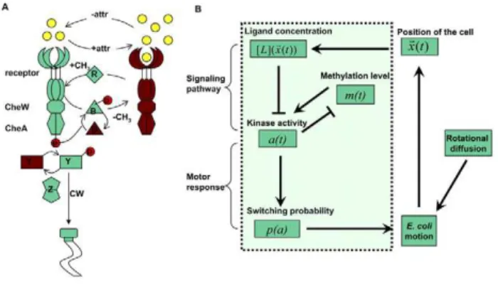
Figure 1. Illustrations of the E. coli chemotaxis pathway and the SPECS (Signaling Pathway-based E. coli Chemotaxis Simulator) model. (A) The E. coli chemotaxis signal transduction
pathway. The MCP complex receptor-CheW-CheA is the sensor and can be active (green) or inactive (dark brown). Binding of attractant molecules (yellow) decreases the probability of the receptor to be active. Once activated, the histidine kinase CheA quickly autopho-sphorylates and then transfers the phosphate group to CheY. CheY-p, the response regulator, diffuses to the flagellar motor and modulates its switching probability between CW and CCW rotations. CheZ, the CheY-p CheY-phosCheY-phatase, serves as the sink of the signal. AdaCheY-ptation of the system is carried out by methylation and demethylation of the receptor, which are facilitated by the enzymes, CheR and CheB-p, respectively. (B) Flow chart of the SPECS model (reproduced from Figure 3 in [21]). The input for the signaling pathway (inside the box) is the instantaneous ligand concentration ½ Lð~xx tð Þ,tÞ. The internal signaling pathway dynamics is described at the coarse-grained level by the interactions between the average receptor methylation levelm tð Þand the kinase activitya tð Þ, which eventually determines the switching probability of the flagellar motor p að Þ. The switching probability is then used to determine the cell motion (run or tumble), and direction of motion during run fluctuates due to rotational diffusion. The motion of the cell leads it to a new location with a new ligand concentration for the cell and the whole simulation process continues.
methylation time scale tm(&1s). The measured CheA auto-phosphorylation time (,0.025s) [25] is also much shorter thantm. Therefore, the kinase activity can be determined by the quasi-equilibrium approximation:
a~ 1
1zexp Nð eðm, L½ ÞÞ: ð1Þ Using the Monod-Wyman-Changeux allosteric model to describe the receptor cooperativity [26,27], the free energy difference can be written as:
eðm,½ LÞ~fmð Þm{ln 1z½ =KAL
1z½ =KIL
, ð2Þ
where fmð Þm is the methylation level-dependent free energy difference;KI andKAare the dissociation constants of the ligand to the inactive and the active receptor, respectively. Quantitative-ly, for MeAsp, which is the chemo-attractant studied here, we use the parameters KI~18:2mM,KA~3mM,N~6 determined by fitting the pathway model to thein vivoFRET data [28]. The free energy contribution due to methylation of the receptor is taken to be linear inm:fmð Þm~aðm0{mÞas used in [15] and supported by recent experiments [29]. The parameters a and m0 can be estimated from the dose-response data [6,30] of the cheRcheB mutants with different methylation levels; for MeAsp, they are roughlya&1:7,m0&1.
The kinetics of the methylation level can be described by the dynamic equation [15]:
dm=dt~F að Þ&kRð1{aÞ{kBa ð3Þ The general methylation rate function F að Þ is expressed by a linear approximation with kR and kB as the linear rates for methylation and demethylation processes. The simple form is based on the assumption that CheR only methylates inactive receptors and CheB-p only demethylates active receptors, which are required to achieve near perfect adaptation in the kinase activity [11,13,14,31]. More complicated Michaelis-Menten equations can be used [32], but they do not affect the results here as the system (pathway) normally operates in the linear range. For simplicity, we take kR~kB to fix the steady state activity a0~0:5; another value a0~1=3was used without affecting the results. The methylation rates can be estimated by the adaptation time from experiments with step function stimuli [4]; for MeAsp, we usekR&0:005=sec. The dependence of the chemotaxis motion onkRis studied in this paper.
Run and tumble motion
A simple phenomenological model is used here to model theE. colicell motion. Lets~0,1represent the tumble and run states of the cell. For the time periodt?tzDt, a cell switches from states to state ð1{sÞ with probability psð½ YÞDt. The response curve measured by Cluzel et al [16] determined the ratio between the two probability rates for one flagellar motor (see Supporting Information (SI) Figure S1 for details on effects of multiple flagella):
p1ð½ YÞ
p0ð½ YÞ
~½ Y
H
Y
½ H0:5, ð4Þ
with H&10 and ½ Y
0:5&3mM. We assume the tumble time is
roughly constant (independent of ½ Y) by setting p0ð½ YÞ~t
{1 0 , where t0&0:2sec. is the average duration of the tumble state. Correspondingly, the probability rate to switch from the run state to the tumble state is:
p1ð ÞY~t
{1 0
Y
½ H
Y
½ H0:5 ð5Þ
In our simulation,½ Y is assumed to be proportional to the kinase activity: ½ Y~Yaa tð Þ without considering the nonlinear depen-dence [33] (Ya is defined later in this paragraph). This linear approximation is justified by the relatively small range of activity variation in our study. Including the CheY-p dephosphorylation dynamics explicitly with dephosphorylation time tz~0:1{0:5s did not significantly change the results (see Figure S1). Spatial effects are neglected as the diffusion time for CheY-p across the cell length is short v50ms [34] and the CheY-p level was measured to be spatially uniform in wtE. colicells [35]. In steady state, a~a0~kR=ðkRzkBÞ and the average run time is t1&0:8sec:. Therefore, Ya is set by Yaa0~½ Y0:5ð0:2=0:8Þ1=H. After a tumbling episode, a new run direction is chosen randomly with the run velocityv0~16:5mm=sec[36]. In our simulations, a small time stepDt~0:1sis chosen to resolve the average tumbling time.
Rotational diffusion
As first pointed out by Berg and Brown [37], one important factor in chemotaxis is the rotational diffusion of the cell due to the Brownian fluctuation of the medium. This can be simply captured by adding a small Gaussian random angledh to the direction of the velocity in every run time stepDt~0:1sec.:
h?hzdh ð6Þ
The amplitude of this rotational diffusion angleDh: ffiffiffiffiffiffiffiffiffiffiffiffiffi Sdh2T q
is roughly 10uas estimated by the fact that it takes,10sec. for the cell to lose its original direction of motion (i.e., turn more than 90u) by pure rotational diffusion.
Boundary effect
For the boundary condition, we assume that when a cell swims to a wall, it swim along the wall for some time (1–5 sec.) before swimming away [21,38]. The boundary condition can affect the cell distribution near the wall, but should not strongly affect the overall behavior of the cell distribution in the bulk.
Results
The SPECS model was used to investigateE. coli chemotaxis behaviors (for individual cells and at the population-level) for a series of ligand profiles with increasing spatial and temporal complexity. Our model revealed the key dynamics of the microscopic control circuit responsible for these behaviors and predicted novel responses to spatio-temporally varying environ-ments, which can be tested by future experiments.
E. colichemotactic motion in stationary ligand gradients: logarithmic sensing and its microscopic mechanism
Constant chemotactic drift velocity in exponential ligand
gradients. One central question in chemotactic motility is
concentration ½ L. We addressed this question by studying cell motion in two types of stationary ligand spatial profiles, linear and exponential, in which the gradient or the relative gradient of the ligand concentration was kept constant, respectively. For an exponential attractant concentration profile ½ L~½ L0exp xð =x0Þ, the relative gradient+½ =L ½ L (or equivalently the gradient of the logarithmic concentration+ln½ L) is a constant vector along the x-direction with magnitudeG:x{01. The response to pure temporal exponential gradient was first studied experimentally by Block et al [39]. Recently, exponential gradient sensing was studied theoretically [15] and from an optimization point of view [19]. Here, by using the SPECS model, we simulated the motion of a population typically consisting of 1000 individuals in different exponential ligand profiles (solid lines, Figure 2A). In comparison, cell motions in linear gradients: ½ L~½ L0ð1zx=x0Þ was also studied (dotted lines, Figure 2B). We calculated the dynamics of the average cell position, the average methylation level, and the average activity of the cells for different values ofx0.
In exponential gradients, the average cell position increases linearly with time, leading to a constant chemotaxis drift velocity vd, before it saturates at a later time. The molecular mechanism for this behavior becomes evident by inspecting the average methylation level of the cells. Initially, as a cell moves up the gradient, its receptor methylation level increases with time to balance the effect of the increasing ligand concentration. This adaptation mechanism maintains the kinase activity within the sensitive range of the flagellar motor and therefore maintains a constant chemotactic drift velocity. Only when the receptor methylation level approaches its maximum value (mmax~4), the chemotactic motion slows because the cell can no longer adapt to higher ligand concentrations, which can be seen in Figure 2A for the case of x0~0:6mm for tw20 min. In contrast, the drift velocity decreases continuously in linear gradients long before the methylation level reaches its maximum (Figure 2B). The difference in drift velocities in exponential and linear gradients originates from the different behaviors in their average kinase activities. In an exponential gradient, the kinase activity shifts to a new steady-state value lower than the perfectly adapted valuea0in the absence of any gradient (Figure 2A). The activity shiftDameasures the kinase response of the cell. The constant kinase responses in exponential gradients lead to constant drift velocities. In a linear gradient, the kinase activity, after an initial fast decrease, continuously recovers towardsa0without reaching a steady state, as shown in Figure 2B. The decreasing kinase response in a linear gradient leads to a decreasing drift velocity (Figure 2B). In Figure 2C, plots of instantaneous drift velocity as a function of ligand concentration for both exponential (solid line) and linear (dotted line) gradients show explicitly that cells move with constant drift velocities in exponential gradients while they slow down in linear gradients as they move to regions with higher ligand concentrations.
The range of ligand concentrations over which the drift velocity remains constant in an exponential gradient is spanned by the two dissociation constants KI and KAðwKIÞ for inactive and active receptors respectively. From Eq. (2), the free energy contribu-tion from ligand binding, fL, can be expressed as: fL~ lnð½ LzKIÞ{lnð½ LzKAÞzlnðKA=KIÞ. Within the rangeKI%
L
½ %KA,fL&lnð½ =KL IÞ. This logarithmic dependence of ligand concentration in the free energy leads to a constant kinase activity shift in response to an exponential temporal gradient [15,39] and eventually results to a constant drift velocity proportional to the gradient of the logarithmic ligand concentration, i.e., the logarithmic sensing behavior. For MeAsp, this range (KA=KI) is over 2 decades as shown in [6,28]. In general, a constant activity shift can be obtained by setting the rate of change in activity free energy to be a constant:LfL=
Lx~x0{1, resulting to the required ligand profile:
L
½ ð Þx ~KA ½ L0expðx=x0Þ {KI
KA{½ L0expðx=x0Þ
, ð7Þ
where the constant½ L0 sets the scale for the ligand concentra-tion. Thus, the required ligand profile is exponential: ½ Lð Þx &
L
½ 0expðx=x0Þas long as½ L is within the range set byKIandKA:
KI%½ L%KA. Recently, Vladimirov et al [20] studied the dependence of drift velocity on gradient shape and adaptation rate with a much smaller range (KA=KI&7) assumed for Asp. A constant drift velocity was reported in [20] for a ligand profile that is quantitatively different from the exponential gradient shown here. This discrepancy is likely caused by the smallerKA=KIratio used in [20]. In addition, an uncontrolled approximation for changes in ligand free energyDfLwas used in [20] to obtain the
Figure 2. Comparison of chemotactic motions in exponential and linear ligand profiles.(A) Cell motion and intracellular dynamics in exponential ligand concentration profiles:½ L~½ L0exp xð=x0Þ. (B) Cell
motion and intracellular dynamics in linear ligand profiles:
L
½ ~½ L0ð1zx=x0Þ. In both (A) & (B), the dynamics of the (population)
averaged position (vxw); the average receptor methylation level (vmw) and the average kinase activity(vaw)are shown for different decay lengthsx0~0:6,1,2,4,8mm.½ L0~3KI. The population-averaged
position increases linearly with time until the methylation level reaches saturation in exponential profiles; while it slows down continuously in the linear profiles. After a transient decrease, the kinase activity stays roughly constant in exponential profiles, while it varies continuously recovering to its pre-stimulus level a0 in linear profiles. (C) Direct comparison of instantaneous velocities between exponential (solid lines) and linear (dotted lines) profiles forx0~0:6mm(black); 1.0 mm (purple). Within the chemosensitivity rangeKIv½ LvKA, the
specific form of ligand profile for constant activity. Linearizing the exponential spatial dependence in the exact solution given in Eq. (7) would lead to a similar (but not identical) spatial gradient form as reported in [20]. However, such linearization is only valid for a limited range of space(x), which is much smaller than the length scalex0of the ligand profile.
The logarithmic sensing behavior, i.e., constant drift velocities in exponential gradients, predicted here from the model can be directly tested by measuring E. coli chemotaxis motion in stationary exponential attractant gradients, which is yet to be achieved experimentally. Recently, we used the SPECS model to simulate E. coli chemotactic motions in a finite channel with different linear ligand profiles. The quantitative agreement with microfluidics experiments [21] indirectly supported the notion that E. coli senses the relative change of ligand concentration and verified the validity of the SPECS model.
Adaptation rate controls the critical exponential gradi-ent and the saturation (maximum) chemotaxis velocity. Within the chemosensitivity range (mvmmax), the average cell positionvxwincreases linearly with time in exponential gradients, resulting in a constant chemotaxis velocityvd:vd:dvxw=dt. The dependence of vd on the exponential gradient G ~x{01
is determined for different values of kR (with fixed kR=kB~1), which correspond to different adaptation rates. As shown in Figure 3A, the drift velocity is linearly proportional to the gradient
of the logarithmic ligand concentration, vd&CG~CLln½L
Lx , for GvGCwhereGCis a critical gradient beyond whichvdsaturates. The linear proportional constantCdefines the chemotaxis motility ofE. colicells and has the dimension of a diffusion constant with its scale set byv2
0t1, wherev0andt1are the average run velocity and run time, respectively. The dimensionless motility constant C*Cv02t1 is directly controlled by the sensitivity of the cell motion to relative ligand concentration changes, and is proportional to the signal amplification at both the receptor and the motor levels. ForGwGC,vdsaturates and becomes independent ofG. This transition depends on the adaptation rate characterized by kR (Figure 3A). Phenomenologically, the chemotaxis velocity for the full range of gradients can be approximately written as:
vd~
CG
1zG=GC
, ð8Þ
and the maximum (saturation) chemotaxis velocity is simply:
vmax~CGC: ð9Þ
Fitting the drift velocities (Figure 3A) with Eq. (8) for different adaptation rates kR, we can quantify the dependence of chemotaxis motion on the adaptation rate. As shown in Figure 3B, the motility constantCis roughly independent ofkR, but the maximum chemotaxis velocityvmax is controlled by the adaptation rate with a scaling dependence vmax*kR0:5. So from Eq. 9, we have:GC!k0R:5.
From Eq. 8, it is clear that GC represents the maximum exponential gradient to which a cell can respond normally (linearly). The scaling dependence ofGC on the adaptation rate
kRcan be understood by the internal signaling pathway dynamics. For a temporal exponential concentration ramp with ramp rater, it was shown in [15] that the kinase activity shifts by a constantDa which is proportional torand the adaptation timetm!1=kR. For a cell moving with a drift velocity vd in a spatial exponential gradient G, the effective average ramp rate it experiences is r~vdG~CG2. Therefore, the kinase activity shift can be obtained
as in [15]:Da~CG2=2ak
R
ð Þ. The flagellar motor responds to the kinase activity within a narrow fixed range of size am&a0=H, whereH&10is the Hill coefficient of the motor response curve [16]. For a givenkR, the adaptation rate is not fast enough to keep the kinase activity within this operational range of the flagellar motor for a very steep gradient, and this critical gradientGC is
Figure 3. Dependence of chemotaxis motion on the adaptation rate. (A) The chemotaxis drift velocity vd for different exponential
gradientG :x{1 0
. Different symbols represent different adaptation rateskR. Note thatvdfirst increases linearly (dashed line) withGbefore
reaching a saturation velocity at a critical gradientGC,. We can fitvd
with:vd~ CG
1zG=GC
, in whichC is the chemotaxis motility constant given by the linear fitting coefficient and the saturation drift velocity is
vmax~CGC. The dependences ofCandvmaxonkRare shown in (B) and
(C) respectively. For the range ofkRwe studied, we found thatCis
roughly independent ofkR and vmax depends on kR with a simple
scaling relation:vmax!k0:5
R .
therefore determined by Da~am, which leads to the observed scaling relation:GC!k1=2
R .
Taken together, a simple coherent picture ofE. colichemotaxis motion emerges from our modeling studies. Within the chemo-sensitive regime (KIv½ vL KA) the chemotaxis drift velocity is linearly proportional to the relative gradient of the concentration. The signal amplification of the underlying pathway increases the chemotaxis motility; and the internal adaptation rate determines the range of this linear response and the maximum drift velocity as summarized in Eq. (8). A few interesting results come directly from this general picture. In a linear gradient½ L~½ L0ð1zx=x0Þ, the dynamics of the averageE. colipositionvxwcan be studied by using Eq. (8) and assuming x{1
0 vGC: dvxw=dt&CG~
C=(vxwzx0), which leads to an analytical solution: vxw~
ffiffiffiffiffiffiffiffiffiffiffiffiffiffiffiffiffi
x2 0z2Ct
q
{x0. This analytical solution agrees with our simula-tion results (Figure 2B). It shows explicitly that the chemotaxis drift motion in a linear gradient is sub-linear with a continuously decreasing velocity and vxw!(Ct)1=2 at long times when
t&x02=C. For a given exponential gradient G, because of the weak dependence of the motility C on kR within the range of adaptation rates we studied, the dependence of the chemotaxis drift velocity onkRdoes not show a pronounced maximum at a particular adaptation rate as reported previously [20]. Instead, the same (near-optimum) chemotaxis velocity is reached, provided that the adaptation ratekRis larger than a minimum ratekR, min to keep the cell within the linear response regime, i.e.,GvGC. From the dependence ofGConkR, we can obtain the dependence ofkR, minonG:kR, min!G2. Of course, extremely fast adaptation with adaptation times approaching the average run time would drastically decrease the drift velocity as the cell loses its ability to distinguish forward runs from backward runs.
Chemotactic motion of individual cells: statistics of the
forward and backward run lengths. In their early work, Berg
and Brown first observed long tracks of E. coli motion and measured the distributions of runs by using a 3D tracking microscope [37]. From the characteristics of the longer runs up the gradient than down the gradient, they first established that bacterial chemotaxis results from longer runs toward attractants. They also found that the distribution of runs down the gradient is similar to the run length distribution in the absence of ligand concentration gradient. This peculiar observation prompted the question of whether the cell only responds to upward the gradient while ignoring the downward gradient. Here, we addressed this question by using our model to study the characteristics of the chemotactic motion of individual cells. We showed the motion of one cell in an exponential ligand gradient profile (x0~4mm) (Figure 4A) and the distributions of the run time in the forward and backward directions (Figure 4B). The average forward run time is longer than the average backward run time, with the distribution of backward run time close to the distribution in the absence of attractant gradient. Our model results are consistent with the experimental observations [37] (Figure 4B inset) without invoking different sensing mechanisms for the downward and upward gradients.
The microscopic mechanism for the run length distributions can be studied with our model. We found that after some initial transient time, the kinase activity fluctuated around a constant average valueSaT. This steady state activity valueSaTwas found to be lower thana0, the steady state activity in the absence of ligand gradient, by an amount that depends on the steepness of the gradient (Figure 4C). This result can be explained as follows. As the cell drifts up the exponential ligand gradient with a constant velocity, the average ligand concentration the cell experiences at time t grows exponentially with t. For an exponential temporal
stimulus, it was first shown experimentally by Block et al [40] that the kinase activity of the cell shifts to a constant value lower than its adapted value. As explained recently in [15], this constant shift in activity is caused by the balance of the exponentially increasing ligand concentration with the linearly increasing methylation level of the receptors. The methylation level versus the logarithmic ligand concentration for individual cells at different times for different exponential gradients collapse onto a universal curve (Figure 4D). The logarithmic external ligand concentration is closely tracked by the receptor methylation level despite the large temporal fluctuations in both these quantities (Figure 4D). Due to the fact thatSaTva0, the overall average of all the run times (both up and down the gradient) is longer than that in the absence of gradient. This also explains the larger cell diffusion constant in the presence of exponential attractant gradients (Figure S2). However, during an individual run down the gradient, the decreasing ligand concentration increases the kinase activity as methylation is too slow to react in the typical run time scale. The opposite is true for the upward run. Indeed, as we examined the kinase activity statistics during the upward and the downward runs separately (Figure 4C), we found that the average kinase activity during downward runsSaTdwas larger than that of the upward runsSaTu:
SaTuvSaTvSaTd. ThereforeSaTdcan approacha0(SaTdcan be smaller or bigger thana0, depending on the methylation rate and ligand gradient) whileSaTandSaTuare always smaller thana0.
Analytically, the activity shift can be obtained by using the results from the last subsection and following the analysis in [15]:
SaT~a0{CG2=2ak
R
ð Þ. The deviation of SaTd and SaTu from
SaTcan be estimated due to slow adaptation during average run time t1:SaTd{SaT~SaT{SaTu&(1{a0)a0NGv0t1=2, which gives: SaTu{a0&{ C
2akR
G2{Nv0t1a0(1{a0)
2 G;SaTd{a0&
{ C
2akR
G2zNv0t1a0(1 {a0)
2 G. These analytical expressions show that while SaTuva0 is always true, SaTdcan be larger, smaller, or equal toa0depending on the exponential gradientG (See Figure S3 in SI for demonstration of all these cases). Quantitatively, the run time distributions depend on the details of the gradient, e.g., the ligand concentration in [37] probably has a Gaussian profile rather than a pure exponential form.
E. colichemotactic motion in oscillating spatial gradients: damped responses at high frequencies
In the natural environment, chemical signals not only vary in space, they also fluctuate in time. The fluctuation of a chemical signal (ligand concentration) sensed by a moving cell can be caused by: 1) randomness in the cell motion, i.e., the run-tumble motion and the rotational diffusion of the cell; and 2) temporal variation of the environment itself. Here, we investigated the effects of the latter due to ligand (spatial) gradients that also vary with time. In particular, based on the feasibility of future experimental tests of our predictions, we studied the case thatE. coliswims in a finite channel of length L where the attractant concentration ½L is linear inside the channel {L=2ƒxƒL=2 with a slope that oscillates in time with a frequencyv:
L
½ ðx,tÞ~g0½sin(vt)xzL=2, ð10Þ with a fixed maximum ligand spatial gradient g0. g0~
due to run-tumble transitions (,1 s) and rotational diffusion (,10 s), we studied the dependence of cell motion on ligand concentration oscillation with relatively low frequencyvv0:1Hz. We found that the average position (center of mass) of theE. coli cells oscillated with the same periodicity as the ligand concentra-tion (Figure 5A). The amplitude of the response depends on the frequency (Figure 5B). For spatial gradients changing with very low frequencies, the response amplitude becomes comparable to the size of the channel and stays almost constant independent ofv due to the boundary effects. For higher frequencies, the amplitude the average cell motion decreases withv. This dependence of cell motion on the frequency of the gradient can be understood by studying the mean-field dynamics of the average position of the cell xc(t) by assuming an instantaneous response to the (logarithmic) ligand gradient:
dxc=dt&C½L{1d½L=dx~ Csin (vt)
sin (vt)xc(t)zL=2
, ð11Þ
whereC is the motility constant defined in the last section. For high frequency, the amplitude of the cell motion is much less than the channel size,DxcD%L=2, and the above equation can be solved approximately to obtain:
xc&2C
Lv(1{cos (vt)), ð12Þ which shows that the response amplitude decreases with frequency as 1=v, consistent with our simulation results (Figure 5B). Equation (12) breaks down and the amplitude saturates at low Figure 4. Single cell behaviors in exponential attractant gradients.(A) Trajectory of a cell for 10 min for½ L~½ L0exp xð=x0Þwithx0~4mm.
The random walk motion is biased towards the gradient (arrow). The forward runs up the gradient are in red, and the backward runs down the gradient are in black. (B) Run length distribution for forward runs (red), backward runs (black) in the presence of an exponential gradient and without a gradient (purple). The backward run length distribution is close to the run length distribution in the absence of a gradient, similar to the experimental results from Berg and Brown [37] as reproduced in the inset. (C) Distributions of cell kinase activity for forward (red) and backward (black) runs. A time series of the activityaof a single cell is shown: forward is in red and backward is in black. The average activity for backward (black dashed line) is closer to the adapted activity (purple dashed line, 0.5) compared with the average activity for forward (red dashed line). (D) Methylation level of different individual cells at different times and in different exponential gradients (represented by color symbols as in Figure 2) all increase with logarithmic ligand concentration along a universal line, despite large temporal fluctuations in methylation levels and positions for (two) individual cells as shown in the inset.
frequenciesvvvl!C=L2, determined by the finite channel size
L(Figure 5B). Quantitatively, the full Eq. (11) does not yield to any simple scaling dependence of response amplitude onv.
How do the adaptation dynamics affect the cell’s response to time-varying gradients? We investigated this question by varying kR (kB was co-varied to keep kR=kB fixed). We found that for smaller values ofkR, a transition frequencyvcappears within the frequency range (v0:1Hz) studied here (Figure 3C). For frequencies higher than vc, the decay in response amplitude became significantly steeper than for frequencies belowvc. The transition frequencyvcis determined by the adaptation rate, with faster rates resulting in highervc(Figure 5C, inset). This transition to faster decay in response amplitude is likely caused by the finite adaptation (response) timeta of the underlying signaling system, which leads to the dependence of the instantaneous drift velocity
on the relative gradients in its past with a exponentially decaying function with time scaleta:
_ x xc(t)&ta
ðt
{?
CLln½L(x,t
0)
Lx |exp ({(t{t
0)=t a)dt0
~
ðt
{?
Ctasin (vt0) exp ({(t{t0)=ta) sin (vt0)x
c(t0)zL=2
dt0:
If the time-dependent term in the denominator of the integrant of the above equation is neglected for small amplitudes of cell motion, we can estimate the amplitude of cell motion at high frequencies: xc&2C
Lv(1{cos (vt))|(1ztav)
{1, which has a
similar time-dependence as in Eq. (12) but with an extra factor (1ztav)
{1due to the finite adaptation time. For high frequencies
vwta{1!kR, this extra factor causes the response amplitude to decay with an extra factor(tav){1, consistent with our simulation results (Figure 5C).
The responses ofE. colito pure temporal oscillatory signals have been studied experimentally [39], theoretically [15], and within the framework of information theory [41]. However, for anE. coli cell moving in a time-varying spatial gradient, its signaling pathway dynamics becomes much more complex as the signal (ligand concentration) changes due to both its temporal and spatial variations convoluted by the cell motion, which is in turn determined by the pathway dynamics. The interplay between spatial and temporal signals coupled to cell motion can lead to rich cellular behaviors, which we have just started to explore. The quantitative dependence of cell motion onvandkRdepends on the details of the ligand spatial profile and a simple analytical form is not available. However, the damped chemotaxis motion in environments with high-frequency gradients should be generally true due to the finite adaptation time of the cell. This frequency-dependent chemotaxis behavior can be tested by future experi-ments in spatial gradients that also change with time with tunable frequencies.
Complex spatial-temporal ligand profile: quantitative simulation of the classical capillary assay
The capillary assay is an ingenious experimental method developed more than a century ago by W. Pfeffer and later perfected by J. Adler’s group to study bacterial chemotaxis [22,23]. A capillary tube containing a solution of attractant is inserted into a liquid medium (the pool) containing bacteria. A gradient of the attractant is subsequently developed due to diffusion and bacterial cells swim into the tube following the gradient. The number of bacteria entering the capillary is counted at a given time (45–60 min), as a measure of the cells’ chemosensitivity. This method is still in use today because of its simplicity and also because the spatiotemporally varying attractant profile mimics the realistic situation of attractant released from a stationary source. Here, we modeled the responses of cells in the capillary assay and quantitatively compared the results with the experimental measurements. The time-dependent attractant concentration was determined by solving the diffusion equations:
LCp
Lt ~DDCp, LCc
Lt ~DDCc, ð13Þ
where Cc and Cp stand for the ligand concentrations in the Figure 5. Responses to oscillating linear gradient. (A) Time
dependence of the average positions of cells for three oscillatory gradients, all with the same amplitude but different frequencies (v). The responses have the same frequencies as their driving signals, but the response amplitude decreases with the driving frequency. (B) The amplitude of the response decreases with frequencyv. The cross-over at low frequency (~4|10{3Hz) is caused by boundary effects. (C)
Upon decreasing adaptation rate, a transition to a steeper decay of the amplitude appears at frequencies higher than a transition frequencyvc
within the range of frequencies studied. Three cases with smaller values ofkR~3|10{4,5|10{4,10{3(s{1)are shown, and the dependence of vcon the adaptation ratekRis shown in the inset of (C).
capillary and the suspension pool respectively.D(&700mm2=s)is the diffusion coefficient of the attractant ligand in water. Using the cylindrical symmetry of the geometry, the ligand concentra-tion was solved in cylindrical coordinates with the boundary conditions:
LCc(zw0,r~R)
Lr ~0,
LCp(z~0,rwR)
Lz ~0,
Cp(z~0,rƒR)~Cc(z~0,rƒR),
ð14Þ
whereR~100mm is the radius of the capillary tube. The initial conditions at t~0 are that the ligand concentrations in the capillary and the suspension pool are C0 and C1 respectively:
Cc(t~0)~C0,Cp(t~0)~C1. The time-dependent concentration profiles are shown in Figure 6A. Starting from beingC1att~0, the ligand concentration at a particular position in the pool peaks at a given time depending on its location (Figure 6A, inset). Furtelle and Berg [42] calculated the attractant profile by solving the diffusion equations asymptotically away from the mouth of the capillary (r~0,z~0), and their analytical asymptotic solution is shown together with our exact numerical solution in Figure 6B at different times along the center line of the capillary tube (r~0). The two solutions show remarkable agreement except for near the mouth of the capillary, where the Furtelle and Berg solution breaks down. Later, we show this inaccuracy near the capillary mouth can cause large differences in computing the result of a capillary assay.
Figure 6. Quantitative simulation of the classical capillary assay and comparison with experiments. (A) Time-dependent ligand concentrations at three different positions in the suspension pool (see inset) from directly solving the ligand diffusion equation. The ligand concentration at a given position peaks at a given time, depending on its location.C0~5mM, C1~0. (B) The exact ligand profile (solid line) along the center line of the capillary at different times, in comparison with the asymptotic solutions (dashed lines) by Furtelle and Berg [42]. (C) Cell density in the rectangular coordinate is shown together with the contours of the logarithmic ligand concentration (inmM) at different times. Three individual cell trajectories (starting from circles and ending at squares) are shown. Only the black cell ends in the capillary. (D) Probability distribution of the original positions of cells that end in the capillary. For a cell originally located at position(r,z), the probability of it ending in the capillary at a later time (45 min),P(r,z), is shown.C0~5mM,C1~0. (E) Concentration-response curve for the capillary assay. The average number of bacteria in the
capillary after 45–50 min subtracted by the number of bacteria in the capillary in the absence of attractant is defined as the response (ordinate). The results from our model with the exact ligand profile are labeled by solid symbols (fitted by a solid line). They agree well with the experimental measurements (hollow squares) of Mesibov et al [22,23]. The results from using the asymptotic ligand profile by Furtelle and Berg are shown by the dashed lines. (F) Response curve for capillary assay withC0=C1~3:16. The solid symbols (fitted with a solid line) represent the model, and the hollow
From the spatial-temporal profile of the attractant, cell motion can be calculated by using SPECS. We considered the bacterial cells started randomly in a region of 2mm|
2mm|2mm around the capillary mouth inside the pool (Figure 6C). The probability P(r,z) of a cell at an original position(r,z)that eventually ends in the capillary at 45min was calculated (Figure 6D). Even cells originally far away from the mouth of the capillary can enter it, withP(r,z)decreasing with both z and r.
Finally, we calculated the chemotactic responses in capillary assay for different values of C0 and/or C1 and compared the results directly with the experiments by Mesibov et al [22,23]. The results showed that the number of bacteria accumulating in the capillary 45 min after the capillary is inserted is a function ofC0 (C1~0) for both the experiments and our simulation (Figure 6E). The results from our model, with no adjustable parameters, agree quantitatively with the experiments. The dashed line in Figure 6E represents the results of our cell motility simulation by using the Furtelle and Berg solution for the ligand concentration. Evidently, even though the Furtelle and Berg solution is accurate away from the capillary mouth, its inaccuracy near the capillary mouth changes the results significantly. The accuracy of the ligand profile near the mouth of the capillary is important because cells that eventually enter the capillary need to pass the mouth. In another set of experiments by Mesibov et al [22], both C0 and C1 are changed while keeping their ratio fixed at C0=C1~3:16. The sensitivity curves are plotted as the number of bacteria accumulating in the capillary after one hour versus (C0C1)1=2 (Figure 6F). The simulation results (filled triangles) showed quantitative agreement with the experiments [17], further verifying our model. Qualitatively, the shape of the capillary assay response can be understood as the chemotaxis response (sensitivity) is small for either very large or very small ligand concentrations. Quantitatively, the peak response concentration is larger than the center of the chemoreceptor sensitivity region [6] due to the fast decay of the ligand concentration from inside the tube toward the pool (Figure 6A).
Discussion
In this paper, a coherent picture of how E. coli chemotaxis motion depends on the spatio-temporally varying chemical environment and its intracellular signaling dynamics has emerged from our modeling study. The chemotaxis drift velocity vd is mainly determined by three factors: vd&FL|FG|Fv, where FL,FG, and Fv depend on the ligand concentration ½L, the gradient of the logarithmic concentrationG~Lln½L=Lx, and the frequency v of the temporal-variation of ½L respectively. For ligand concentrations within a wide (chemosensitive) range KIv½LvKA (as focused on in this paper), the concentration-dependent factorFL&1, andvddepend linearly on the gradient of the logarithmic concentrationGuntil it saturates at a high rela-tive gradient GwGC as demonstrated by the second factor
FG&CG=(1zG=GC). For a ligand gradient that varies with high frequency vwvC, vd is damped by the third factor
Fv&(1zv=vC){1due to the finite adaptation time(ta!v{C1) in the underlying signaling pathway. We found that the saturation gradient GC is controlled by the adaptation rate kR, but the motility constant C is not (although weak dependence on kR cannot be completely ruled out). The nontrivial scaling depen-dence GC!k1R=2, observed in our simulation, can be explained analytically by the dynamics of the internal signaling pathway and the narrow range of kinase activity over which the flagellar motor can response.
Calibrated quantitatively by the most up-to-date in vivoFRET experiments, our model (SPECS) captures the essential character-istics of the underlying signaling network, in particular the receptor-receptor cooperativity and the near-perfect adaptation kinetics, within a simple unified mathematical description. We described the internal state of a cell at the coarse-grained (cellular) level without modeling the details of individual signaling molecules as used in other simulation methods such as StochSim [17], AgentCell [18], and E. solo [10], which are particularly suited to studying noise in the intracellular signaling process. This coarse-grained approach, similar to that used in RapidCell [20], greatly reduces the computational requirements for the simulation. For example, the SPECS model allows us to simulate E. coli populations of 103–104 cells in a linear ligand concentration profile and 102–103cells in a capillary assay in real timewith a standard desktop computer (Matlab code available upon request); and the simulation results agree quantitatively with both the recent microfluidics experiments and the classical capillary assay measurements, without any fitting parameters. Predictions, such as bacterial chemotactic responses in exponential ligand profiles and oscillatory ligand gradients, are made with our model and can be tested by future experiments. Indeed, the SPECS model can be used to predict E. coli chemotaxis motions in arbitrary spatial-temporal varying environments efficiently and accurately.
Perhaps equally important as predicting cellular behaviors, the SPECS model, which captures the essential features of the underlying pathway, enables us to understand these behaviors based on the key intracellular signaling dynamics, some of which can be difficult to study directly by experimental methods. For example, the constant drift velocity in an exponential ligand profile was found to be caused by a constant shift in the average kinase activity, which is maintained by a linearly increasing mean methylation level in balancing the exponentially increasing ligand concentration. At the individual cell level, this constant activity shift is also shown to be responsible for the intriguing observation that the average backward run time in an exponential gradient is similar to the average run time in the absence of a gradient, while the forward run time is much longer.
The SPECS model can be used to study various noise effects as well. The effect of the cell-to-cell variability for chemotaxis behavior in a linear gradient in a closed channel was studied by choosing (from a broad distribution) a random value for the internal parameters such as N, methylation rate constants, and swimming velocity in each individual cell. We found that although individual cells now behaved differently, at the population level, the average steady state behavior, such as cell density, remained almost the same (see Figure S4) except for a slight change near the boundary for the case with run velocity variation. The main source of (external) temporal noise for the cell’s chemotactic sensory system comes from the run and tumble motion of the cell. Even in a smooth spatial ligand gradient, the randomness in the cell motion can lead to large temporal fluctuations in the input (ligand concentration) to the E. coli’s chemotactic sensory system. This source of external noise was included in our model. The effects of fluctuations in intracellular signaling remain to be examined. By adding noise to our pathway model, it would be interesting to see whether and how the internal signaling noise affects the population level behavior.
between the cells and the liquid-solid surface were oversimplified in this paper. Cells are known to turn with a preferred handedness when they run into a surface [43] and can remain near the surface for a long time [38] before they finally escape. It would be interesting to see how different ‘‘boundary conditions’’ affect the overall behavior of cells. In its natural environment, a cell must make decisions in the presence of multiple, sometimes conflicting cues. Our model can be extended to include integration between different chemotactic signals [26] and applied to study bacterial motion in the presence of multiple stimuli gradients. The same chemotaxis pathway seems to be able to sense and react to other non-chemical stimuli, such as temperature [44] and osmotic pressure [45]. Our model can be modified to study the responses of cells to these non-chemical stimuli by incorporating the dependence of various (kinetic and energetic) biochemical parameters on the strength of these external stimuli. Recently, we carried out such extensions to study the microscopic mechanism of precision-sensing inE. colithermotaxis [46]. Finally, the chemo-attractant (MeAsp) considered in this paper is non-metabolizable and its concentration gradient is formed indepen-dent of the cell population. In other cases, such as in swarm plate experiments [47], the attractant gradient is generated by consumption of the nutrient, which is also the chemo-attractant. In addition, cells can communicate by emitting chemo-attractants
[48]. The consumption and generation of the attractant, together with cell division, need to be incorporated into our model to understand complex pattern formations in different swarm plate experiments. We are currently pursuing some of these directions.
Supporting Information
Figure S1 Effects of CheY-p dephosphorylation and multiple
motors.
Found at: doi:10.1371/journal.pcbi.1000735.s001 (0.06 MB PDF)
Figure S2 Chemotactic drift velocity and diffusion constant in
exponential ligand concentration gradients.
Found at: doi:10.1371/journal.pcbi.1000735.s002 (0.06 MB PDF)
Figure S3 Single cell behavior in different exponential gradients.
Found at: doi:10.1371/journal.pcbi.1000735.s003 (0.04 MB PDF)
Figure S4 Effects of cell-to-cell variability.
Found at: doi:10.1371/journal.pcbi.1000735.s004 (0.06 MB PDF)
Author Contributions
Conceived and designed the experiments: QO YT. Performed the experiments: LJ YT. Analyzed the data: LJ QO YT. Wrote the paper: LJ QO YT.
References
1. Sourjik V (2004) Receptor clustering and signal processing in E.coli chemotaxis. Trends Microbiol 12: 569–576.
2. Stock J, Re SD (2000) Chemotaxis Lederberg J, Alexander M, Bloom B, Hopwood D, Hull R, et al., eds. San Diego, CA: Academic Press. pp 772–780. 3. Bren A, Eisenbach M (2000) How signals are heard during bacterial chemotaxis: protein-protein interactions in sensory propagation. J Bacteriol 182: 6865– 6873.
4. Berg HC, Tedesco PM (1975) Transient response to chemotactic stimuli in Escherichia coli. Proc Natl Acad Sci USA 72: 3235–3239.
5. Segall JE, Block SM, Berg HC (1986) Temporal comparisons in bacterial chemotaxis. Proc Natl Acad Sci USA 83: 8987–8991.
6. Sourjik V, Berg HC (2002) Receptor sensitivity in bacterial chemotaxis. Proc Natl Acad Sci USA 99: 123–127.
7. Bray D, Levin MD, Morton-Firth CJ (1998) Receptor clustering as a cellular mechanism to control sensitivity. Nature 393: 85–88.
8. Duke TAJ, Bray D (1999) Heighted sensitivity of a lattice of membrane receptors. Proc Natl Acad Sci USA 96: 10104–10108.
9. Mello BA, Tu Y (2003) Quantitative modeling of sensitivity in bacterial chemotaxis: The role of coupling among different chemoreceptor species. Proc Natl Acad Sci USA 100: 8223–8228.
10. Bray D, Levin MD, Lipkow K (2007) The chemotactic behaviors of computer-based surrogate bacteria. Curr Biol 17: 12–19.
11. Barkai N, Leibler S (1997) Robustness in simple biochemical networks. Nature 387: 913–917.
12. Alon U, Surette MG, Barkai N, Leibler S (1999) Robustness in bacterial chemotaxis. Nature 397: 168–171.
13. Yi T-M, Huang Y, Simon MI, Doyle J (2000) Robust perfect adaptation in bacterial chemotaxis through integral feedback control. Proc Natl Acad Sci USA 97: 4649–4653.
14. Mello BA, Tu Y (2003) Perfect and near-perfect adaptation in a model of bacterial chemotaxis. Biophys J 84: 2943–2956.
15. Tu Y, Shimizu TS, Berg HC (2008) Modeling the chemotactic response of Escherichia coli to time-varying stimuli. Proc Natl Acad Sci USA 105: 14855–14860.
16. Cluzel P, Surette M, Leibler S (2000) An ultrasensitive bacterial motor revealed by monitoring signaling proteins in single cells. Science 287: 1652–1655. 17. Morton-Firth CJ, Bray D (1998) Predicting temporal fluctuations in an
intracellular signaling pathway. J Theor Biol 192: 117–128.
18. Emonet T, Macal CM, North MJ, Wickersham CE, Cluzel P (2005) AgentCell: a digital single-cell assay for bacterial chemotaxis. Bioinformatics 21: 2714–2721. 19. Andrews BW, Yi TM, Iglesias PA (2006) Optimal noise filtering in the chemotactic response of Escherichia coli. PLoS Comput Biol 2: e154. doi:110.1371/journal.pcbi.0020154.
20. Vladimirov N, Løvdok L, Lebiedz D, Sourjik V (2008) Dependence of bacterial chemotaxis on gradient shape and adaptation rate. PLoS Comput Biol 4: e1000242. doi:1000210.1001371/journal.pcbi.1000242.
21. Kalinin YV, Jiang L, Tu Y, Wu M (2009) Logarithmic sensing in Escherichia coli bacterial chemotaxis. Biophys J 96: 2439–2448.
22. Mesibov R, Ordal GW, Adler J (1973) The range of attractant concentrations for bacteria chemotaxis and the threshold and size of receptor over this range Weber law and related phenomena. J Gen Physiol 62: 203–223.
23. Mesibov R, Adler J (1972) Chemotaxis toward amino acids in Escherichia coli. J Bacteriol 112: 315–326.
24. Biemann HP, Koshland DE, Jr. (1994) Aspartate receptors of Escherichia coli and Salmonella typhimurium bind ligand with negative and half-of-the-sites cooperativity. Biochemistry 33: 629–634.
25. Francis NR, Levit MN, Shaikh TR, Melanson LA, Stock JB, et al. (2002) Subunit organization in a soluble complex of Tar, CheW, and CheA by electron microscopy. J Biol Chem 277: 36755–36759.
26. Mello BA, Tu Y (2005) An allosteric model for heterogeneous receptor complexes: Understanding bacterial chemotaxis responses to multiple stimuli. Proc Natl Acad Sci USA 102: 17354–17359.
27. Keymer JE, Endres RG, Skoge M, Meir Y, Wingreen NS (2006) Chemosening in Escherichia coli: two regimes of two-state receptors. Proc Natl Acad Sci USA 103: 1786–1791.
28. Mello BA, Tu Y (2007) Effects of adaptation in maintaining high sensitivity over a wide range of backgrounds for Escherichia coli chemotaxis. Biophys J 92: 2329–2337.
29. Vaknin A, Berg HC (2007) Physical responses of bacterial chemoreceptors. J Mol Biol 366: 1416–1423.
30. Shimizu TS, Delalez N, Pichler K, Berg HC (2006) Monitoring bacterial chemotaxis by using bioluminescence resonance energy transfer: absence of feedback from the flagella motors. Proc Natl Acad Sci USA 103: 2093–2097. 31. Brown DA, Berg HC (1974) Temporal stimulation of chemotaxis in Escherichia
coli. Proc Natl Acad Sci USA 71: 1388–1393.
32. Emonet T, Cluzel P (2008) Relationship between cellular response and behavioral variability in bacterial chemotaxis. Proc Natl Acad Sci USA 105: 3304–3309.
33. van Albada SB, Ten Wolde PR (2009) Differential affinity and catalytic activity of CheZ in E. coli chemotaxis. PLoS Comput Biol 5: e1000378.
34. Sourjik V, Berg HC (2002) Binding of the E. coli response regulator CheY to its target is measured in vivo by fluorescence resonance energy transfer. Proc Natl Acad Sci USA 99: 12669–12674.
35. Vaknin A, Berg HC (2004) Single-cell FRET imaging of phosphatase activity in the Escherichia coli chemotaxis system. Proc Natl Acad Sci USA 101: 17072–17077.
36. Alon U, Camarena L, Surette MG, Arcas BAy, Liu Y, et al. (1998) Response regulator output in bacterial chemotaxis. EMBO J 17: 4238–4248.
37. Berg HC, Brown DA (1972) Chemotaxis in Escherichia coli analyzed by three-dimensional tracking. Nature 239: 500–504.
38. Frymier PD, Ford RM, Berg HC, Cummings PT (1995) Three-dimensional tracking of motile bacteria near a solid planar surface. Proc Natl Acad Sci USA 92: 6195–6199.
39. Block SM, Segall JE, Berg HC (1983) Adaptation kinetics in bacterial chemotaxis. J Bacteriol 154: 312–323.
41. Tostevin F, ten Wolde PR (2009) Mutual information between input and output trajectories of biochemical networks. Phys Rev Lett 102: 218101.
42. Futrelle RP, Berg HC (1972) Specification of gradients used for studies of chemotaxis. Nature 239: 517–518.
43. DiLuzio WR, Turner L, Mayer M, Garstecki P, Weibel DB, et al. (2005) Escherichia coli swim on the right-hand side. Nature 435: 1271–1274. 44. Mizuno T, Imae Y (1984) Conditional inversion of the thermoresponse in
Escherichia coli. J Bacteriol 159: 360–367.
45. Vaknin A, Berg HC (2006) Osmotic stress mechanically perturbs chemorecep-tors in Escherichia coli. Proc Natl Acad Sci USA 103: 592–596.
46. Jiang L, Ouyang Q, Tu Y (2009) A mechanism for precision-sensing via a gradient-sensing pathway: a model of Escherichia coli thermotaxis. Biophys J 97: 74–82.
47. Budrene EO, Berg HC (1995) Dynamics of formation of symmetrical patterns by chemotactic bacteria. Nature 376: 49–53.