Testing APT Model upon a BVB Stocks’ Portfolio
Alexandra BONTAŞ1, Ioan ODĂGESCU2
1
Romanian National Securities Commission, Bucharest, Romania
2
Academy of Economic Studies, Bucharest, Romania [email protected], [email protected]
Applying the Arbitrage Pricing Theory model (APT), there can be identified the major factors of influence for a BVB’ portfolio stocks’ trend. There were taken into consideration two of the APT theory models, establishing influences upon portfolio’s yield: given to macroeconomic environment and to some stochastic factors. The research’s results certify that, on the long term, what influences the stocks’ movement in the stock market is mostly the action of specific short-term factors, without general covering, like the ones that are classified in the research area of behavioral finance (investors’ preference towards risk and towards time).
Keywords: Portfolio, Risk, Stocks, Yield, Testing
Introduction
For covering risk, it is necessary to ana-lyze the relation risk-yield of financial in-struments available for investment, in order to make the investment decision one rational. The allocation of the resources decision to-wards a stocks’ portfolio is direct influenced by their yield. This yield can be analyzed by taking the past performances (historic per-formances) of the financial instruments and the predicted performances (expected antici-pated for the future). Based on own expecta-tions, each investor establishes a level of ex-pected yield (requested yield) for each of the investment opportunity, this yield including a series of factors like the inflation rate, eco-nomic growth, consumption prices index, in-terest etc. Between the economic growth rate, that requires a decline of the inflation rate, a strengthening of the national currency in comparison with different universal traded currencies etc., and the investment opportuni-ties exists a close relation, in the way that the investors’ requested yield must be at least equal with the economic growth rate (the economy’s expansion provokes the growth of the number and the value of the investment opportunities).
The risk premium that an investor is willing to assume must cover all the possible risks, the investor identifying himself with those specific risk factors. This premium is seen by the investors as being direct proportional with their investment’s yield (once the risk
grows, also the risk premium grows, and is necessary to rise the investment’s yield in or-der to ensure a full cover of the risk). The risk of a financial instrument refers, in this way, to the financial instruments yields’ volatility and to the investment’s perception upon results’ uncertainty.
2 Arbitrage Pricing Theory Model For covering risks, it is necessary to imple-ment a risk – yield report for the financial in-struments available for an investment, in or-der to make the investment decision one ra-tional [1]. The decision to reserve resources to a financial portfolio is directly influenced by the portfolio’s financial instruments yield. This yield can be analyzed through past per-formances (historical) of the financial in-struments and through the predicted perfor-mances (expected, anticipated for the future). Depending on own expectations, each inves-tor establishes an expected level of yield (re-quested yield) for each investment opportuni-ty, and this yield includes a series of factors like inflation rate, economic growth, con-sumer prices index, interest rate and so on [2]. Between the economic growth, that im-plies a fall of the inflation rate, a strengthen of the national currency in relation to other universal traded currencies etc, and the in-vestment opportunities there is a tighten rela-tionship, in the sense that the yield requested by the investors must be at least equal to the economic growth rate (the economy’s
sion provoke the growth of the number and value of the investment opportunities). The risk premium that an investor is willing to assume must cover possible risks, the in-vestor identifying himself with the specific risk factors. The risk premium is seen by the investors as being directly proportional with their investments’ yield (once the risk grows, and so the risk premium grows, it is neces-sary for covering the poverty to exist a growth in the investments’ yield). The risk of a financial instrument refers at the volatility of those instruments’ yield and at the invest-ment perception over the results uncertainty [3].
The APT Model (Arbitrage Pricing Theory) is one of the models most recommended to be used in financial portfolio’s optimization [4], depending on the relationship between the risk and the yield. The general hypothe-ses of the APT models are:
- the factorial models can explain the
fi-nancial yields; in other words, by select-ing a number of factors, it can be ex-plained the evolution of the markets;
- the arbitrage opportunities represent, in
fact, portfolios without investments, as there is necessary inside this portfolios to exist some perfect hedging operations;
- the arbitrage opportunities appear when
the unique price rule is broken; the inex-istence on the real market of such a price drives to the existence of some arbitrage opportunities between different financial instruments or different trading places;
- the financial markets are characterized
through a high volatility; the permanent fluctuation of the prices is given by the
investors’ reaction towards different in-fluence factors, that can be, by their na-ture, of many types (economic, social, psychological etc.) or can be perceived by the investors, and so by the market through its general evolution, in different proportions (the importance of the influ-ence factors for each investor or market differs); breaking the existing principles for the arbitrage conditions is a clear form of irrationality on the market;
- the rational equilibrium of the market is
the effect of the pressures made by the arbitrage opportunities; the results of such opportunities do not depend on the risk aversion.
In order to find the factors that can explain the best the yields of the financial instru-ments, we have tested the APT models of Chen, Ross and Roll and of Morgan Stanley. For the chosen models there were used finan-cial market’s and real economy’ indicators for the period 2003-2008, taking into consid-eration a portfolio of 10 stocks traded on Bu-charest Stock Exchange (B.V.B.), considered to be blue-chips: SIF1 (SIF Banat-Crişana), SIF2 (SIF Moldova), SIF3 (SIF Transilvania), SIF4 (SIF Muntenia), SIF5 (SIF Oltenia), and the 5 stocks that go into BET basket (the general index of B.V.B.), re-spectively SNP (Petrom), BRD (Groupe Societé Generale), TLV (Banca Transilvania), AZO (Azomureş), RRC (Rompetrol Rafinare) [5].
To quantify risk, the following statistical in-dicators can be used:
- variance (σ
2
- medium square defiance), calculated with the formula:
−
=−
= − = = − = n i si
R
iE
R
ip
i nR
iE
R
iR E R E 1 2 1 2 2 2
)]
(
[
)]
(
[
* 11)] ( [
σ
- standard deviation (σ), calculated with the formula σ = √σ2;
- variance coefficient (CV), calculated with
the formula:
) (R E CV = σ
;
- semi variance (semiVar): semiVar(R) =
E[R*]2, where R* = min[R-E(R); 0].
where:
s = number of states (registrations);
n= number of observations from the consid-ered series of yields (for a series of historical yields); formula for the yield is the average of distribution
== s
i i i
i
R
p
R
E
1 * )
(
(pi is the probability in
sate i).
From the virtual portfolio’ financial instru-ments’ distributions, for the period of time analyzed (daily series of data for 01.01.2003-31.12.2008), it can be observed a relative normal distribution (symmetric), the values being situated on both sides of the class with the maximum effective are relatively equal, or differing relatively little (normal distribu-tion law).
Starting from the models’ hypothesis, it was followed to explain the portfolio stocks’ yield through the factors considered by each tested model. Both tested models have differ-ent factors, in this way being tried to cover as many influence possibilities for the yield as much as possible. The portfolio stocks’ yields have been calculated, on the basis of the closing prices, for the time period 01.01.2003-31.12.2008, according to the formula:
Yield = (Price at the end of the month – Price at the beginning of the month)/Price at the beginning of the month
The risk preference taken into consideration in testing the chosen models was calculated as a difference between the stocks open-end funds’ yield (as being considered with the highest level of risk) and the money-market open-end funds’ yield (as being considered with the lowest level of risk). The yield for the open-end funds (FDI) has been calculated on the monthly data series for the period 2003-2008, according to the formula:
FDI Yield = ln (Actual monthly medium val-ue of the unit fund / Previous monthly medi-um value of the unit fund)
The time preference taken into consideration in testing the chosen models has been calcu-lated as the difference between the stocks’ open-end funds’ yield and the fix revenue’ open-end funds’ yield (for the HT indicator – high time, long term), respectively the differ-ence with the money market’ open-end funds’ yield (for the LT indicator – low time, short term), the formula of time preference
being obtained, on the basis of monthly data series for the period 2003-2008, according to the formula:
Time Pref. = HT – LT
3 Testing the portfolio with the APT mod-el Chen, Ross and Roll
Starting from the Chen, Ross and Roll APT model, it can be observed that the financial instruments’ yields on the capital market de-pend on the following factors:
- industrial production (reflects changes in
the expectations related to the cash flows);
- difference of yield between the
corpora-tive with low risk and those with high risk (changes in the investors’ risk pref-erence);
- difference between the short term interest
rate (TS) and the long term one (TL) (changes in investors’ time preference);
- un-anticipated inflation; - anticipated inflation.
Taking into consideration the available data, we’ve tested an adjusted form of the APT model of Chen, Ross and Roll, that includes inflation instead of un-anticipated and antici-pated inflation, industrial production (noted with PINDUST), the difference of yield be-tween the corporative bonds with low risk and those with high risk (as an expression of risk preference; noted with RISCPREF), the difference between the short term interest rate and the long term interest rate (as an ex-pression of time preference; noted with TIMEPREF).
The general equation used is:
Stock = C(1) * PINDUST + C(2) * RISCPREF + C(3) * TIMEPREF + C(4) * INFLATION + ε
where: C(1), C(2), C(3), C(4) are coefficients given to the influence factors (factor’s sensi-bility), and ε is the risk.
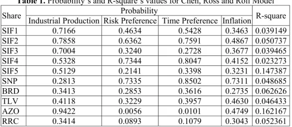
Table 1. Probability’s and R-square’s values for Chen, Ross and Roll Model
Share Probability R-square
Industrial Production Risk Preference Time Preference Inflation
SIF1 0.7166 0.4634 0.5428 0.3463 0.039149
SIF2 0.7858 0.6362 0.7591 0.4867 0.050737
SIF3 0.7004 0.3240 0.2728 0.3677 0.039465
SIF4 0.5328 0.7344 0.8047 0.4152 0.023273
SIF5 0.5129 0.2141 0.3398 0.3231 0.147387
SNP 0.2813 0.7335 0.8502 0.7311 0.048685
BRD 0.3413 0.2853 0.3616 0.2735 0.062626
TLV 0.4118 0.3229 0.3957 0.4630 0.046433
AZO 0.9422 0.0056 0.0101 0.4749 0.162167
RRC 0.3414 0.0893 0.1079 0.3043 0.052361
Table 2. Regression coefficients’ values for Chen, Ross and Roll Model
Share Coefficients
Industrial Production Risk Preference Time Preference Inflation
SIF1 -0.002310 2,009,907 -1,656,402 2,579,542
SIF2 -0.001768 1,324,805 -0,853060 1,946,416
SIF3 -0.002568 -2,821,864 3,161,019 2,587,325
SIF4 -0.003808 0,889990 -0,644222 2,137,268
SIF5 -0.004792 3,929,112 -2,992,741 3,112,851
SNP -0.005495 0,743817 -0,409983 0,749439
BRD -0.005042 2,445,521 -2,074,078 2,495,861
TLV -0.005397 2,798,655 -2,387,088 2,070,790
AZO 0.000469 7,929,593 -7,287,427 1,988,604
RRC -0.007360 5,695,060 -5,347,955 3,413,429
Applying the obtained results from Table 1 and Table 2, the estimated equations become: SIF1 = -0.002310074588 * PINDUST + 2.009907344 * RISCPREF – 1.65640249 * TIMEPREF + 2.579542263 * INFLATION +
ε
SIF2 = -0.001768459305 * PINDUST + 1.324804855 * RISCPREF – 0.8530602313 * TIMEPREF + 1.946416221 * INFLATION + ε
SIF3 = -0.002568469315 * PINDUST – 2.821863517 * TIMEPREF + 3.161018678 * RISCPREF + 2.587324941 * INFLATION +
ε
SIF4 = -0.003807643417 * PINDUST + 0.8899898697 * RISCPREF – 0.644222161 * TIMEPREF + 2.137268037 * INFLATION + ε
SIF5 = -0.004791674586 * PINDUST + 3.929112249 * RISCPREF – 2.992741479 *
TIMEPREF + 3.112851376 * INFLATION +
ε
SNP = -0.005494624743 * PINDUST + 0.7438166006 * RISCPREF – 0.4099827055 * TIMEPREF + 0.7494393582 * INFLA-TION + ε
TLV = -0.00539681391 * PINDUST + 2.798654605 * RISCPREF – 2.387087802 * TIMEPREF + 2.07078993 * INFLATION +
ε
BRD = -0.005042411472 * PINDUST + 2.445521353 * RISCPREF – 2.074078204 * TIMEPREF + 2.495860683 * INFLATION +
ε
AZO = 0.000469346612 * PINDUST + 7.92959265 * RISCPREF – 7.287426535 * TIMEPREF + 1.988604207 * INFLATION +
ε
TIMEPREF + 3.41342949 * INFLATION +
ε
The obtained data, as seen in Table 2 draw attention to the R-square. This represents a statistical measure that shows in which way (as good as possible) a regression line ap-proximates the data real points (a value of R-square over 1, respectively 100%, indicates a perfect match).
The formula applicable for this value is:
r(X,Y) = [Cov(X,Y)] / [StdDev(X) * StdDev(Y)]
When applying this indicator in finance, R-square measures the proportion in which a model can predict or explain the actual per-formances of an investment or of a portfolio of financial instruments. As closer is its the value to 1, as much the portfolio’s financial instruments’ yield depends on the factors taken into consideration by the model.
From Table 2 it can be observed that the val-ues of the statistical indicator R-square are very small, without being closet o the level of 100% (unit value), for neither of the financial instruments selected for the portfolio.
The first conclusion that comes out is that there is a very weak relationship between the portfolio’s stocks’ yields and the influence factors (industrial production, risk prefer-ence, time preferprefer-ence, and inflation). There-fore, the prices of the instruments cannot be explained through the perspective of these factors (as not being influenced by this com-bination of factors).
Also, it can be observed a probability higher than 0.05 (5%) of the factors considered by the model (the optimum probability for these factors to be relevant is 95%). In this way can be drawn a second conclusion, that the considered model, through its selected fac-tors, is not relevant for measuring the yield for the portfolio and for its stocks.
In the case of data presented in Table 2, we can also observe the direct and inverse pro-portionality of the coefficients considered by the model towards the stocks’ yield. The ex-istence of negative coefficients shows an
in-verse influence of the coefficients over the stocks, namely if their values are positive there is a direct proportional influence. In the case of testing the portfolio by this model it can be observed that:
- the industrial production influences in a
reverse way the stocks’ yield (with an ex-ception - AZO, that responds to the in-dustrial production trend);
- the risk preference influences directly the
stocks’ yield (with the exception of SIF3, which stocks can be traded by the moder-ate risk investors);
- time preference influences in a reverse
way the stocks’ yield (with the exception of SIF3, being preferable to invest on long term in this stock);
- inflation influences in a reverse way the
stocks’ yield (without any exception). The lack of direct proportional relations be-tween the industrial production, inflation and time preference and the stocks’ yields, and also the lack of reverse proportionality rela-tions between risk preference and stocks’ yield (between risk aversion and the growth of prices for a stock there must be a direct proportional relationship) show (as a third conclusion) that the stocks’ prices do not de-pend on the sum of these factors.
4 Testing the portfolio with the APT mod-el Morgan Stanley
Taking into consideration the conclusions of the testing applied to APT model Chen, Ross and Roll over the virtual portfolio’s stocks’ yield, we have tested another APT model. Starting from the hypothesis of APT model Morgan Stanley, the financial instruments’ yields on the capital market depends on the following factors:
- GDP’s growth;
- long term interest rate;
- exchange rate (as a currency basket); - market factor;
- consumer prices index (IPC) or the prices
index for petroleum goods.
model with a linear regression equation, in which the independent variables are:
- interest rate (represented by the interest
rate applicable at bank credits);
- exchange rate (CSV – a currency basket
formed by Euro - 80% and US dollar - 20%);
- market factor (represented by BET index
of B.V.B.);
- inflation, used as an adjusted form that
took into consideration inflation instead
of un-anticipated or anticipated inflation (inflation rate = IPC – 100).
The applied equation is:
Stock = C(1) * INTEREST + C(2) * CSV + C(3) * BET + C(4) * INFLATION +ε
In the testing of this model, the values ob-served for the dependent variables are pre-sented in the next tables:
Table 3. Probability’s and R-square’s values for Morgan Stanley Model
Shares Probability R-square
Interest CSV BET Inflation
SIF1 0.8317 0.1221 0.3938 0.5166 0.059407 SIF2 0.8736 0.1127 0.2731 0.7742 0.071520 SIF3 0.9507 0.1654 0.4375 0.7209 0.047628 SIF4 0.9448 0.1788 0.5511 0.5761 0.042711 SIF5 0.6409 0.3469 0.0066 0.5573 0.131706 SNP 0.8795 0.0059 0.5037 0.5921 0.128760 BRD 0.8107 0.0207 0.2741 0.4662 0.110009 TLV 0.4468 0.3216 0.3694 0.6568 0.047679 AZO 0.3671 0.0385 0.2966 0.6019 0.082609 RRC 0.0932 0.0598 0.8231 0.0956 0.066698
Table 4. Regression coefficients’ values for Morgan Stanley Model
Shares Coefficients
Interest CSV BET Inflation SIF1 -0.039810 -1.631.944 0.151352 3.056.758 SIF2 0.030473 -1.712.928 0.199271 1.381.288 SIF3 -0.012232 -1.542.850 0.145406 1.775.976 SIF4 -0.012433 -1.357.916 0.101308 2.525.870 SIF5 -0.102516 -1.157.739 0.579673 3.242.586 SNP -0.021929 -2.289.173 0.091560 1.949.063 BRD -0.037224 -2.024.626 0.160181 2.836.657 TLV 0.148731 -1.083.996 0.166000 -2.180.100 AZO -0.182298 -2.366.596 0.199601 2.644.254 RRC -0.386316 -2.425.996 0.048115 9.635.849
The estimated equations are:
SIF1 = -0.03980993813*INTEREST - 1,631944066*CSV + 0,1513519589*BET + 3.056758137*INFLATION +ε
SIF2 = 0.03047261264*INTEREST – 1.712928377*CSV + 0.1992712824*BET + 1.381287745*INFLATION +ε
SIF3 = -0.01223239692*INTEREST – 1.542850064*CSV + 0.1454059768*BET +
1,775975719*INFLATION +ε
SIF4 = -0.01243266517*INTEREST – 1.357916093*CSV + 0.1013078093*BET + 2.525870211*INFLATION +ε
SIF5 = -0.1025161647*INTEREST – 1.157738713*CSV + 0.5796725389*BET + 3.242586292*INFLATION +ε
1.94906333*INFLATION +ε
BRD = -0.03722386141*INTEREST – 2.024625511*CSV + 0.1601808093*BET + 2.836656783*INFLATION +ε
TLV = 0.1487314609*INTEREST – 1.083996437*CSV + 0.1659999085*BET – 2.180099781*INFLATION +ε
AZO = -0.1822983759*INTEREST – 2.36659587*CSV + 0.1996006543*BET + 2.64425428*INFLATION +ε
RRC = -0.3863164573*INTEREST – 2.425996486*CSV + 0.04811531515*BET + 9.635849435*INFLATION +ε
The obtained data, as seen in Table 3, draws attention over the R-square index (with the same formula and the same statistical signifi-cance from the previous model) and it can be observed that the values of R-square are smaller also for this model, without being close to the level of 100% (unit value), for neither of the portfolio’s selected financial instruments.
The fourth conclusion is that neither in this model, there is no strong connection between the stocks’ yields and the influence factors considered (credits’ interest rate, exchange rate, BET index, inflation). Therefore, in this case too, the prices of the financial instru-ments selected in the portfolio cannot be ex-plained from the point of view of the influ-ence factors (as not being influinflu-enced by this combination of factors).
Moreover, it can be observed that neither in this model there is a probability over 0.05 (5%) of the considered factors (the difference towards the optimum probability shows that the chosen factors are not relevant). It can be drawn a fifth conclusion, that the model con-sidered, through its factors, is not relevant to measure the portfolio’s yield or its stocks’ yields.
In the case of the data presented in Table 4, it can be observed the direct and reverse pro-portional influence of the coefficients con-sidered by the model towards the stocks’ yields, namely:
- the interest rate influence in a reverse
way the stocks’ yield (with the exception of SIF2 and TLV);
- the exchange rate (CSV) influences in a
reverse way the stocks’ yield;
- BET and inflation influence directly
pro-portional the stocks’ yield (with the ex-ception of TLV in the case of inflation). Normally, the interest rate, the exchange rate and the stock exchange index should influ-ence in a direct proportional way the stocks’ yields, namely their growth should have as an effect the growth of the yields. The eco-nomic factors selected offer a growth or a fall of the risk premium accepted by the investor that modifies the expected yield of his in-vestment, making his preference to be orien-tated to certain financial instruments or cer-tain prices or yields available. The growth in credit interest rate and in exchange rate make the investor to look for a higher yield for his stock exchange investments (in this case, stocks from the portfolio), and therefore pro-voking the generalized growth of market prices (quotations) (the relation price/yield must include the growth supported by the vestor and created by the growth of credit in-terest rate, exchange rate or inflation rate). If for the index BET of B.V.B. one can say that there is a direct proportional relationship with the statistical data regarding the selected stocks’ yields (which is normal, considering that in the selected portfolio are 5 of the 10 blue-chips from BET), for the other factors there is no such relation of normality.
The lack of direct proportionality relation be-tween the stocks’ yield and the credit interest rate and exchange rate and the lack of reverse proportionality relation between stocks’ yield and inflation show (a sixth conclusion) that the stocks’ prices do not depend on the sum of factors considered by the APT model Morgan Stanley.
5 Virtual portfolio test using the adjusted APT Model
also the market’s evolution factors, and therefore the lack of correlation rises a seri-ous question).
Taking into consideration that both APT models tested before didn’t presented a sig-nificant relevance for the selection of influ-ence factors, the conclusions that were drawn after testing the Chen, Ross and Roll model and the Morgan Stanley model over the vir-tual portfolio stocks’ yield didn’t gave an ex-planation for the yield in the analyzed period (2003-2008). Therefore, it was necessary to test, on the same data series, other models of the same type, but with a different combina-tion of factors.
A set of seven factors (from the ones before analyzed) were chosen (industrial production, risk preference, time preference, inflation, in-terest rate for credits, exchange rate and BET-C index of B.V.B.), in order to detect a certain structure that can offer a relationship between them, and to permit a classification by importance and relevance over the stocks’ yield. Generating a case with multiple varia-bles ensures the defining of a space in which the stocks’ yield depends upon the influence factors.
The composing method of the factors was re-alized based on the principal component analysis principle (generated with the SPSS software), as this method is the most appro-priate for the case in which, for a set of vari-ables observed, one can whish for selecting a group of other artificial variables (principal components), that will sum together with the biggest variance of the initial factors’ set.
The components resulted (influence factors) have the capacity to be used as prognosis fac-tors or criteria variables in the present tests. Through this method it is applied the proce-dure of reducing the variables.
The analyze used in composing the factors within the method chosen is based on an in-dependent sample (the virtual portfolio creat-ed), with more than two independent varia-bles (multivariate analyses) and has as objec-tive the measuring of the association level and the central determination, respectively the evaluation of the significance of the dif-ferences between the variables and the groups of variables (causality relationship of the sample and the variables).
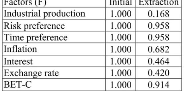
Following the before analyzed models, other two models were built for testing: F1 and F2. For testing of these two, seven factors of in-fluence were taken, as mentioned above, and, starting from correlations equal to 1 between the factors included in the analyze, it result-ed, after the extract based on principal com-ponents analyses, in a set of indicators differ-ently correlated, in connection to their rele-vance in the actual testing. From the obtained data, as shown in Table 5, it can be observed that, in this model, the highest relevance for the dynamic of the portfolio selected stocks’ yield is given for the risk preference, the time preference and BET-C index.
The obtained data are sustained by the dy-namics that the stocks’ prices had in the ana-lyzed period (2003-2008) and by the invest-ment behavior.
Table 5. Selection method for factors by its relevance (relevance test – scree plot test) Factors (F) Initial Extraction
Industrial production 1.000 0.168 Risk preference 1.000 0.958 Time preference 1.000 0.958
Inflation 1.000 0.682
Interest 1.000 0.464
Exchange rate 1.000 0.420
BET-C 1.000 0.914
The communality represents the explained proportion of factors from the variance of a variable. Because the tries are correlations
de-termination coefficient (R2), if the variable is predicted by components. It can be computed the communality of a variable as sum of tries’ squares on variables. The initial com-munalities are equal to 1, being calculated before reducing the dimension.
The factors tries (the extraction column) rep-resents the base of the factors’ naming, an important problem in factorial analysis. A
factor, as passive variable, must have a name that can be understood, used, referred to and so on. The loading structure of a factor can offer suggestions in this sense, as tries bigger than 0.6 are considered being important, and as those with a value under 0.4 are consid-ered as being small. The variables with big tries constitute the initial variables’ combina-tion that determines the factor.
own values
0 0,5 1 1,5 2 2,5 3 3,5
1 2 3 4 5 6 7
component factors
Fig. 1. Scree plot test
Table 6 shows in which proportion the total variance can be explained by the factors in-cluded in the analysis. An important point is that of establishing the number j of principal components that will be kept in the final model (the relevance test – scree plot test). It can be observed that the first three factors explain the total variance in a proportion of
78.763% (summed up), and that the first two explain the total variance in a proportion of 65.211% (summed up). The direction change of the curve that takes place after factor 3 shows the low relevance of the previous fac-tors, namely from factor 3 to factor 7, as seen in Fig. 1.
Table 6. Total variance explanation
F
Initial own value Extraction of square tries sums*
Rotation of square tries sums*
total variance %
cumulative
% total
variance %
cumulative
% total
variance %
cumulative % 1 3.038 43.395 43.395 3.038 43.395 43.395 2.998 42.836 42.836 2 1.527 21.816 65.211 1.527 21.816 65.211 1.566 22.375 65.211
3 .949 13.552 78.763 - - - -
4 .906 12.942 91.705 - - - -
5 .465 6.645 98.350 - - - -
6 .113 1.613 99.963 - - - -
7 .003 0.037 100.000 - - - - - -
* square structures = squared loadings, method of computing the relevance of a factor by comparing to a struc-ture from which it belongs (weight in total strucstruc-ture, variance towards the total strucstruc-ture or towards the rest of components’ parts of the structure) depending on its weight in a total of many factors.
The explained variance for each component after the rotation is equal to the tries’ square sum, contributing to the decision regarding the number of components that must be kept, the sum of the tries’ squares (SSL, sum of squared loadings) after rotation being some-how similar to own value. As a result, it can be kept those components with a post-rotation SSL higher as value than 1, the smaller values not being calculated anymore (are not presenting a significance).
The own value table (eigen values) contains, besides the effective value, the necessary cal-culation for identifying the explained vari-ances of the components. The sum of the seven own values is equal to 7 (number of variables). The variance proportion explained by a component is represented by the ratio between the own value and 7 (reminding that each own value represents the explained var-iance, captured by the component). The ini-tial own value under a cumulative form (cu-mulative %) shows directly how much of the total variance is explained by retaining a number of components.
Extracting the following data (sums of the square structures and their rotation) of the factors 3-7 is no longer relevant, due to the initial own values obtained for the seven var-iables (influence factors).
The extraction’s results of two principal components out of the seven indicators are presented in Table 7, named also the “
Com-ponent Matrix” (loading matrix, factor pat-tern matrix). Essentially for the analyses, this contains the loading of the factors (factor loadings); the matrix‘s elements (tries) repre-sents the correlations between components (columns) and the initial variables (rows). Given the components’ proprieties (that are octagonal), the tries have also the interpreta-tion of standardized coefficients from the multiple regression, in other words it shows with how many standard defiance sx is
modi-fied x, if the factor modifies with a standard defiance sF.
The columns shows how each of the selected influence factors is correlated with the two components previous selected (risk prefer-ence and time preferprefer-ence). A negative rela-tion indicates the reverse proporrela-tionality be-tween the two values, namely a positive rela-tion for a direct proporrela-tionality. Therefore it can be observed that if the risk preference grows, this can be realized simultaneous with the growth of time preference and of the val-ue of BET-C index (a valval-ue close to 1 indi-cates a strong connection).
There exist, also, a weak relation (values close to 0) between risk preference and in-dustrial production, inflation and exchange rate. Regarding the time preference, this is directly proportional with the inflation, change rate and interest rate, proving the ex-istence of a strong relation, more pronounced in the case of inflation.
Table 7. Extracting two principal components
Components Risk preference Time preference
Industrial production -0.086 -0.401
Risk preference 0.970 -0.130
Time preference 0.970 -0.128
Inflation 0.218 0.796
Interest 0.419 0.537
Exchange rate -0.141 0.633
BET-C 0.951 -0.099
Interpreting the extraction on two compo-nents determines exactly how much of each element is measured by each. It exist more validation conditions (interpretation) for the method’s preciseness that shows if the
hy-pothesis of the selected models F1 and F2 started from just rationalities:
- the existence of three variables (factors)
components;
- the three variables of each component are
into the same group of significance (risk preference, time preference and BET-C are inter-connected/inter-dependent, the same as in the case of inflation, exchange rate and interest rate);
- the groups of significance for the
compo-nents differ (component 1 means the in-vestment behavior, and component 2 means the macro-economic evolution);
- there is a rotation in the significance of
the factors, similar to applying the first matrix (there are three important factors, followed by other factors with lower rel-evance) for each of the two components. The validation criteria for the selection are fulfilled and results into the validation of the selection of factors, namely in rolling over the F1 and F2 models, in a similar way as the APT models tested before, for the set of sev-en factors available.
The equations used for applying the APT models F1 and F2 are:
F1: Stock = C(1) * F1 + C(2) * C(2) + ε F2: Stock = C(1) * F2 + C(2) * C(2) + ε where:
C(1) and C(2) are the coefficients from the regression equation, with C(1) referring to factors and C(2) being the free coefficient from the equation.
The coefficient C(2) can catch any factor dif-fered by F1/F2 care that could estimate the yield if we consider it not equal to 0. If C(2) = 0, there is no other factor that could influ-ence the yield (false hypothesis), and there-fore results that the relevance for the situa-tion in which C(2) is not equal to zero (C(2)
≠ 0).
The observed values for the dependent varia-bles used in testing models F1 and F2 are shown in Tables 8 and 9:
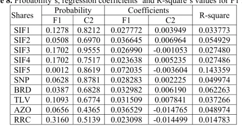
Table 8. Probability’s, regression coefficients’ and R-square’s values for F1 Model
Shares Probability Coefficients R-square
F1 C2 F1 C2
SIF1 0.1278 0.8212 0.027772 0.003949 0.033773 SIF2 0.0508 0.6970 0.036645 0.006964 0.054929 SIF3 0.1702 0.9555 0.026990 -0.001053 0.027480 SIF4 0.1702 0.7517 0.023638 0.005235 0.027486 SIF5 0.0012 0.8619 0.072035 -0.003604 0.143359 SNP 0.0628 0.8781 0.028283 0.002225 0.049974 BRD 0.0387 0.6828 0.032982 0.006190 0.062263 TLV 0.1093 0.6774 0.031509 0.007841 0.037266 AZO 0.0656 0.4365 0.036529 -0.014765 0.048974 RRC 0.3160 0.5139 0.023098 -0.014499 0.014783
The estimated equations for F1 model appli-cation are:
SIF1 = 0.02777243616 * F1 + 0.003949133658 * 0.003949133658 + ε
SIF2 = 0.03664496421 * F1 + 0.006964251883 * 0.006964251883 + ε
SIF3 = 0.02698956254 * F1 – 0.001053087384 * -0.001053087384 + ε
SIF4 = 0.02363826219 * F1 + 0.005235076144 * 0.005235076144 + ε
SIF5 = 0.07203472967 * F1 – 0.00360409364 * -0.00360409364 + ε
SNP = 0.0282825186 * F1 +
0.002225304096 * 0.002225304096 + ε
TLV = 0.03150888512 * F1 + 0.007840719662 * 0.007840719662 + ε
BRD = 0.03298205378 * F1 + 0.006189695552 * 0.006189695552 + ε
AZO = 0.03652911693 * F1 – 0.01476540284 * -0.01476540284 + ε
RRC = 0.02309836327 * F1 – 0.0144985722 * -0.0144985722 + ε
rele-vance but not significant from the point of view of the intensity, as the intensity of the relation is low (between the portfolio stocks’ yield and the influence factors). Including in the model of all influence factors (seven) shows a diminishing of the values of R-square obtained in the previous testing of the APT models (Chen, Ross and Roll and Mor-gan Stanley), and therefore can be drawn a first conclusion: the stocks’ yields have a lowest intensity relation when the seven fac-tors are being composed than when they are taken separate (on categories, in the APT model), and that means a statistical rele-vance.
Moreover, it can be observed a probability for F1 close to the value 0.05 (5%) for the factors in the model, but also a probability of C(2) bigger than the value 0.05. it can be dis-tinguished a second conclusion, that certain factors included in the F1 model (risk prefer-ence, time preference and BET-C index) are relevant for measuring the portfolio’s yield, and meantime the other four factors do not present a significant relevance level. Con-cerning the value of the coefficients F1 and C(2), it can be observed that these are mostly positive, therefore they influence directly
proportional the stocks’ yield, and the values of C(2) are very small, and therefore it results a minimum influence of the excepted factors in F1 model.
In the case of F2 model testing, the estimated equations are built by using the coefficients of this model, as seen in Table 9:
SIF1 = -0.006230405343 * F2 + 0.004949647681 * 0.004949647681 + ε
SIF2 = -0.008771980149 * F2 + 0.008264870718 * 0.008264870718 + ε
SIF3 = -0.003841895182 * F2 – 2.353266977e-006 * -2.353266977e-006 + ε SIF4 = -0.01503962467 * F2 + 0.005741591933 * 0.005741591933 + ε
SIF5 = -0.0166121183 * F2 – 0.00102503038 * -0.00102503038 + ε
SNP = -0.02281187421 * F2 + 0.002660610306 * 0.002660610306 + ε
BRD = -0.02267601181 * F2 + 0.006453528296 * 0.006453528296 + ε
TLV = 0.0184444501 * F2 + 0.009880011983 * 0.009880011983 + ε
AZO = -0.003991768683 * F2 – 0.01330047014 * -0.01330047014 + ε
RRC = 0.02210412035 * F2 – 0.01269944283 * -0.01269944283 + ε
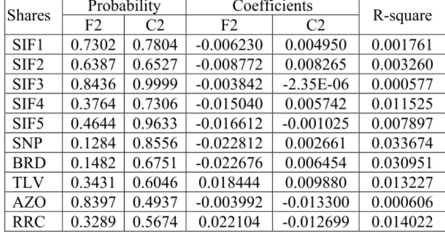
Table 9. Probability’s, regression coefficients’ and R-square’s values for F2 Model
Shares Probability Coefficients R-square
F2 C2 F2 C2
SIF1 0.7302 0.7804 -0.006230 0.004950 0.001761 SIF2 0.6387 0.6527 -0.008772 0.008265 0.003260 SIF3 0.8436 0.9999 -0.003842 -2.35E-06 0.000577 SIF4 0.3764 0.7306 -0.015040 0.005742 0.011525 SIF5 0.4644 0.9633 -0.016612 -0.001025 0.007897 SNP 0.1284 0.8556 -0.022812 0.002661 0.033674 BRD 0.1482 0.6751 -0.022676 0.006454 0.030951 TLV 0.3431 0.6046 0.018444 0.009880 0.013227 AZO 0.8397 0.4937 -0.003992 -0.013300 0.000606 RRC 0.3289 0.5674 0.022104 -0.012699 0.014022
From the obtained data presented in Table 9, it can be seen that neither in this model’s case, R-squared doesn’t have values close to 1, therefore the same type of conclusions can be drawn as in the previous model case (F1). But, in this case, the F2 probability is not close to the value 0.05, and therefore no
strong connection between stocks’ yield and F2 influence factors is observed. Also, the F2 coefficients are mostly negative, showing a reverse proportionality relationship towards stocks’ yield.
6 Conclusions
cover-ing risk, it is a must, in the light of establish-ing the foundation of a rational investment decision, to analyze the risk-yield relation as-sociated to the portfolio’s stocks. Taking into consideration the national stock market par-ticularities, we have considered that the most appropriate model (from the correctness of the applicability point of view) for testing the built portfolio is APT (Arbitrage Pricing Theory).
After testing the portfolio by using the APT Chen, Ross and Roll Model and Morgan Stanley Model, we have noticed that there is an atypical reaction of the financial instru-ments from the portfolio towards the factors of influence considered by the models. The two tested models used different factors, try-ing to cover as much as possible the influ-ence possibilities of the yield, but the test-ing’s result showed that none of these two models can explain the selected portfolio stocks’ yield, being hard to estimate an eco-nomic based relationship between the histori-cal yields (2003-2008) of the shares and ref-erence economic indicators.
The obtained result’s irrelevance, considering the influence factors, determined the necessi-ty of testing the portfolio by a re-combined set of factors, on the same series of dates and a similar estimation model. Other two APT models were built (F1 and F2), that had as in-fluence factors a set of seven from before an-alyzed ones (industrial production, risk pref-erence, time prefpref-erence, inflation, interest rate for credits, exchange rate and BET-C in-dex from B.V.B.). Applying the composing model by principal component analysis prin-ciple, it was looked for detecting a certain structure that could offer a relationship be-tween influence factors, taking into consider-ation their relevance towards the evolution of the portfolio’s yield. From the gained infor-mation and data it can be observed that the highest influence towards the yield’s dynam-ic is settled by the risk preference and the time preference of the investors, in other words one can observe the existence of an investment herd behavior, deeply specula-tive, despite the investment behavior orien-tated towards economic substantiation of the
financial decision [6]. In fact, it is revealed that the stocks’ prices movement is existing as an effect of an investment decision with-out rationality and withwith-out a long term fi-nancing perspective, given only by the ”feel-ing” of certain ”market makers”, speculative type [7]. The selection made was then tested, the validation criteria being fulfilled and a correct selection being generated.
The testing conclusion for the two APT mod-els F1 and F2 is that, in both cases, these are statistical relevant but not relevant from the point of view of the relationship’s intensity between stocks’ yield and the influence fac-tors, the low intensity showing that neither of the factors can explain, without any doubt, the stocks from the selected portfolio yield. Anyway, in the case of F1 model, the proba-bility’s values are close to the level of 0.05 and, in comparison to the same values ob-tained by testing the APT models Chen, Ross and Roll, Morgan Stanley and F2, these val-ues are the most favorable to testing, existing the conclusion that, from all seven selected factors, the ones that can influence most sig-nificant the stocks yield are the risk prefer-ence, the time preference and BET-C index. The previous conclusion, according to which one can say that there is an atypical evolution of the stocks yield, sustains the lack of corre-lation between the stocks’ yield and the in-fluence factors from the APT models, no matter if these are specific to the stock ex-change or of macro-economic type [8]. Only characteristic factors for the investment be-havior are the ones that respond to the appli-cation of the APT models, in different pro-portions.
References
[1] E. Fama and M. H. Miller, “The Theory of Finance”, Hinsdale: Dryden Press, 1972.
[2] L. Glosten, R. Jagannathan and D. Runkle, “On the Relation between the Expected Value and the Volatility of the Nominal Excess Return on Stocks”, Ox-ford: Journal of Finance, 1993, vol. 48, nr. 5.
[3] C. N. Jr. Rosemberg, “Stock Market Pri-mer”, New York: Warner Books Inc., 1991.
[4] J. Knight, “Forecasting Volatility of Fi-nancial Market”, Oxford: Elsevier Press, 2007.
[5] S. Levy and M. Sarnat, “Portfolio and In-vestment Selection: Theory and Prac-tice”, New Jersey: Prentice Hall, 1984. [6] L. Modigliani and F. Modigliani,
“Risk-Adjusted Performance”, New York: Journal of Portfolio Management, 1997. [7] D. Easley, M. López de Prado and M.
O'Hara, “Flow Toxicity and Volatility in a High Frequency World”, Johnson School Research Paper, series no. 9-2011, 2010.
[8] G. Baltussen, “Behavioral Finance: An Introduction”, Social Science Research
Network, http://ssrn.com/abstract =1488110, 2009.
Alexandra BONTAŞ is a specialist within Romanian National Securities Commission since 2003. She holds a PhD in Economy, financial specializa-tion since 2010, author of a series of articles. Graduate numerous naspecializa-tional and international seminaries and participate in several national and interna-tional conferences.