Sensitivity Analysis in Practice

(1)

(2)

(3)

(4)

SENSITIVITY ANALYSIS

IN PRACTICE

A GUIDE TO ASSESSING

SCIENTIFIC MODELS

Andrea Saltelli, Stefano Tarantola,

Francesca Campolongo and Marco Ratto

(5)

Telephone (+44) 1243 779777

Email (for orders and customer service enquiries): [email protected] Visit our Home Page on www.wileyeurope.com or www.wiley.com

All Rights Reserved. No part of this publication may be reproduced, stored in a retrieval system or transmitted in any form or by any means, electronic, mechanical, photocopying, recording, scanning or otherwise, except under the terms of the Copyright, Designs and Patents Act 1988 or under the terms of a licence issued by the Copyright Licensing Agency Ltd, 90 Tottenham Court Road, London W1T 4LP, UK, without the permission in writing of the Publisher. Requests to the Publisher should be addressed to the Permissions Department, John Wiley & Sons Ltd, The Atrium, Southern Gate, Chichester, West Sussex PO19 8SQ, England, or emailed to [email protected], or faxed to (+44) 1243 770571.

This publication is designed to provide accurate and authoritative information in regard to the subject matter covered. It is sold on the understanding that the Publisher is not engaged in rendering professional services. If professional advice or other expert assistance is required, the services of a competent professional should be sought.

Other Wiley Editorial Offices

John Wiley & Sons Inc., 111 River Street, Hoboken, NJ 07030, USA Jossey-Bass, 989 Market Street, San Francisco, CA 94103-1741, USA Wiley-VCH Verlag GmbH, Boschstr. 12, D-69469 Weinheim, Germany

John Wiley & Sons Australia Ltd, 33 Park Road, Milton, Queensland 4064, Australia John Wiley & Sons (Asia) Pte Ltd, 2 Clementi Loop #02-01, Jin Xing Distripark, Singapore 129809

John Wiley & Sons Canada Ltd, 22 Worcester Road, Etobicoke, Ontario, Canada M9W 1L1

Wiley also publishes its books in a variety of electronic formats. Some content that appears in print may not be available in electronic books.

Library of Congress Cataloging-in-Publication Data

Sensitivity analysis in practice : a guide to assessing scientiﬁc models / Andrea Saltelli. . .[et al.].

p. cm.

Includes bibliographical references and index. ISBN 0-470-87093-1 (cloth : alk. paper)

1. Sensitivity theory (Mathematics)—Simulation methods. 2. SIMLAB. I. Saltelli, A. (Andrea), 1953–

QA402.3 .S453 2004 003′_.5—dc22 _2003021209

British Library Cataloguing in Publication Data

A catalogue record for this book is available from the British Library

ISBN 0-470-87093-1 EUR 20859 EN

Typeset in 12/14pt Sabon by TechBooks, New Delhi, India Printed and bound in Great Britain

(6)

PREFACE

This book is a ‘primer’ in global sensitivity analysis (SA). Its am-bition is to enable the reader to apply global SA to a mathematical or computational model. It offers a description of a few selected techniques for sensitivity analysis, used for assessing the relative importance of model input factors. These techniques will answer questions of the type ‘which of the uncertain input factors is more important in determining the uncertainty in the output of interest?’ or ‘if we could eliminate the uncertainty in one of the input factors, which factor should we choose to reduce the most the variance of the output?’ Throughout this primer, the input factors of interest will be those that are uncertain, i.e. whose value lie within a finite interval of non-zero width. As a result, the reader will not find sensitivity analysis methods here that look at the local property of the input–output relationships, such as derivative-based analysis1. Special attention is paid to the selection of the method, to the fram-ing of the analysis and to the interpretation and presentation of the results. The examples will help the reader to apply the methods in a way that is unambiguous and justifiable, so as to make the sensitiv-ity analysis an added value to model-based studies or assessments. Both diagnostic and prognostic uses of models will be considered (a description of these is in Chapter 2), and Bayesian tools of anal-ysis will be applied in conjunction with sensitivity analanal-ysis. When discussing sensitivity with respect to factors, we shall interpret the term ‘factor’ in a very broad sense: a factor is anything that can be changed in a model prior to its execution. This also includes struc-tural or epistemic sources of uncertainty. To make an example, factors will be presented in applications that are in fact ‘triggers’, used to select one model structure versus another, one mesh size ver-sus another, or altogether different conceptualisations of a system.

(11)

Often, models use multi-dimensional uncertain parameters and/or input data to deﬁne the geographically distributed properties of a natural system. In such cases, a reduced set of scalar factors has to be identiﬁed in order to characterise the multi-dimensional un-certainty in a condensed, but exhaustive fashion. Factors will be sampled either from their prior distribution, or from their posterior distribution, if this is available. The main methods that we present in this primer are all related to one another and are the method of

Morris for factors’ screening and variance-based measures2_{. Also}

touched upon are Monte Carlo ﬁltering in conjunction with either a variance based method or a simple two-sample test such as the Smirnov test. All methods used in this book are model-free, in the sense that their application does not rely on special assumptions on the behaviour of the model (such as linearity, monotonicity and additivity of the relationship between input factors and model output).

The reader is encouraged to replicate the test cases offered in this book before trying the methods on the model of inter-est. To this effect, the SIMLAB software for sensitivity analy-sis is offered. It is available free on the Web-page of this book http://www.jrc.cec.eu.int/uasa/primer-SA.asp. Also available at the

same URL are a set of scripts in MATLABr _{and the GLUEWIN}

software that implements a combination of global sensitivity anal-ysis, Monte Carlo ﬁltering and Bayesian uncertainty estimation.

This book is organised as follows. The ﬁrst chapter presents the reader with most of the main concepts of the book, through their application to a simple example, and offers boxes with recipes to replicate the example using SIMLAB. All the concepts will then be revisited in the subsequent chapters. In Chapter 2 we offer another preview of the contents of the book, introducing succinctly the examples and their role in the primer. Chapter 2 also gives some deﬁnitions of the subject matter and ideas about the framing of the sensitivity analysis in relation to the defensi-bility of model-based assessment. Chapter 3 gives a full descrip-tion of the test cases. Chapter 4 tackles screening methods for

2_{Variance based measures are generally estimated numerically using either the method of Sobol’}

(12)

(13)

(14)

1

A WORKED EXAMPLE

This chapter presents an exhaustive analysis of a simple example, in order to give the reader a ﬁrst overall view of the problems met in quantitative sensitivity analysis and the methods used to solve them. In the following chapters the same problems, questions, and techniques will be presented in full detail.

We start with a sensitivity analysis for a mathematical model in its simplest form, and work it out adding complications to it one at a time. By this process the reader will meet sensitivity analysis methods of increasing complexity, starting from the elementary approaches to the more quantitative ones.

1.1 A simple model

A simple portfolio model is:

Y =CsPs+CtPt+CjPj (1.1)

whereY is the estimated risk1 _in_€_,_C

s, Ct, Cj are the quantities per item, and Ps, Pt, Pj arehedgedportfolios in€.2This means that each Px, x = {s,t, j} is composed of more than one item – so that the average return Pxis zero€. For instance, each hedged portfolio could be composed of an option plus a certain amount of underlying stock offsetting the option risk exposure due to

1_{This is the common use of the term.}_Y_{is in fact a return. A negative uncertain value of}_Y_is

what constitutes the risk.

2_{This simple model could well be seen as a composite (or synthetic) indicator camp by}

aggre-gating a set of standardised base indicatorsPiwith weightsCi(Tarantolaet al., 2002; Saisana

and Tarantola, 2002).

(15)

movements in the market stock price. Initially we assume

Cs, Ct, Cj = constants. We also assume that an estimation pro-cedure has generated the following distributions for Ps,Pt,Pj:

Ps ∼ N( ¯ps, σs), p¯s =0, σs =4

Pt ∼ N( ¯pt, σt), p¯t =0, σt =2

Pj ∼ Np¯j, σj, p¯j =0, σj =1.

(1.2)

The Pxs are assumed independent for the moment. As a result

of these assumptions, Y will also be normally distributed with

parameters

¯

y=Csp¯s+Ctp¯t+Cjp¯j (1.3)

σy=

C2

sσs2+Ct2σt2+C2jσj2. (1.4)

Box 1.1 SIMLAB

The reader may want at this stage, or later in the study, to get started with SIMLAB by reproducing the results (1.3)–(1.4). This is in fact an uncertainty analysis, e.g. a characterisation

of the output distribution of Y given the uncertainties in its

input. The ﬁrst thing to do is to input the factors Ps,Pt,Pj with the distributions given in (1.2). This is done using the left-most panel of SIMLAB (Figure 7.1), as follows:

1. Select ‘New Sample Generation’, then ‘Conﬁgure’, then ‘Create New’ when the new window ‘STATISTICAL PRE PROCESSOR’ is displayed.

2. Select ‘Add’ from the input factor selection panel and add factors one at a time as instructed by SIMLAB. Select ‘Ac-cept factors’ when ﬁnished. This takes the reader back to the ‘STATISTICAL PRE PROCESSOR’ window.

(16)

4. Go back to the left-most part of the SIMLAB main menu and click on ‘Generate’. A sample is now available for the simulation.

5. We now move to the middle of the panel (Model execution) and select ‘Conﬁgure (Monte Carlo)’ and ‘Select Model’. A new panel appears.

6. Select ‘Internal Model’ and ‘Create new’. A formula parser appears. Enter the name of the output variable, e.g. ‘Y’ and follow the SIMLAB formula editor to enter Equation (1.1) with values ofCs, Ct, Cj of choice.

7. Select ‘Start Monte Carlo’ from the main model panel. The model is now executed the required number of times.

8. Move to the right-most panel of SIMLAB. Select ‘Anal-yse UA/SA’, select ‘Y’ as the output variable as prompted; choose the single time point option. This is to tell SIMLAB that in this case the output is not a time series.

9. Click on UA. The ﬁgure on this page is produced. Click on the square dot labelled ‘Y’ on the right of the ﬁgure and

read the mean and standard deviation ofY. You can now

(17)

Let us initially assume that Cs< Ct < Cj, i.e. we hold more of the less volatile items (but we shall change this in the follow-ing). A sensitivity analysis of this model should tell us something about the relative importance of the uncertain factors in Equation

(1.1) in determining the output of interest Y, the risk from the

portfolio.

According to ﬁrst intuition, as well as to most of the existing literature on SA, the way to do this is by computing derivatives, i.e.

Sd

x =

∂Y

∂Px

,with x=s,t,j (1.5)

where the superscript ‘d’ has been added to remind us that this

measure is in principle dimensioned (∂Y/∂Pxis in fact dimension-less, but∂Y/∂Cxwould be in€). ComputingSd_x for our model we obtain

S_xd=Cx,with x=s,t,j. (1.6)

If we use the Sd

xs as our sensitivity measure, then the order of

importance of our factors isPj > Pt > Ps, based on the assumption

Cs <Ct <Cj. Sdx gives us the increase in the output of interestY

per unit increase in the factor Px. There seems to be something

wrong with this result: we have more items of portfolio j but this

is the one with the least volatility (it has the smallest standard deviation, see Equation (1.2)). Even ifσs≫σt, σj, Equation (1.6) would still indicatePj to be the most important factor, asYwould be locally more sensitive to it than to either Pt or Ps.

Sometime local sensitivity measures are normalised by some ref-erence or central value. If

y0 =Csps0+Ctp0t +Cjp0j. (1.7)

then one can compute

Sl_x= p

0

x

y0

∂Y

∂Px

(18)

Applying this to our model, Equation (1.1), one obtains:

Sl_x=Cx

p0

x

y0,with x=s,t,j. (1.9)

In this case the order of importance of the factors depends on the relative value of theCxs weighted by the reference values px0s.

The superscript ‘l’ indicates that this index can be written as a

logarithmic ratio if the derivative is computed in p0

x. Sl x= p0 x y0 ∂Y

∂Px

_y₀

,p0 x

= ∂ln (Y)

∂ln (Px)

_y₀

,p0 x

. (1.10)

Sl_x gives the fractional increase inY corresponding to a unit frac-tional increase in Px. Note that the reference point ps0,pt0,p0j might be made to coincide with the vector of the mean val-ues ¯ps,p¯t,p¯j, though this would not in general guarantee that

¯

y= Y( ¯ps,p¯t,p¯j), even though this is now the case (Equation (1.3)). Since ¯ps,p¯t,p¯j =0 and ¯y=0, S_xl collapses to be identical to Sd

x. AlsoSl

xis insensitive to the factors’ standard deviations. It seems

a better measure of importance than Sd

x, as it takes away the di-mensions and is normalised, but it still offers little guidance as

to how the uncertainty in Y depends upon the uncertainty in the

Pxs.

A ﬁrst step in the direction of characterising uncertainty is a nor-malisation of the derivatives by the factors’ standard deviations:

Sσ s =

σs σy

∂Y

∂Ps

=Cs

σs σy Sσ t = σt σy ∂Y

∂Pt

=Ct

σt σy (1.11) Sσ j = σj σy ∂Y

∂Pj

=Cj

σj σy

where again the right-hand sides in (1.11) are obtained by applying Equation (1.1). Note thatSd

(19)

Table 1.1 Sσ

x measures for model (1.1) and different values ofCs,Ct,Cj (analytical values).

Cs,Ct,Cj = Cs,Ct,Cj = Cs,Ct,Cj= Factor 100, 500, 1000 300, 300, 300 500, 400, 100

Ps 0.272 0.873 0.928

Pt 0.680 0.436 0.371

Pj 0.680 0.218 0.046

need no assumption on the range of variation of a factor. They can be computed numerically by perturbing the factor around the base value. Sometimes they are computed directly from the solution of a differential equation, or by embedding sets of instructions into

an existing computer program that computes Y. Conversely, Sσ

x needs assumptions to be made about the range of variation of the factor, so that although the derivative remains local in nature, Sσ

x is a hybrid local–global measure.

Also when using Sσ

x, the relative importance of Ps, Pt, Pj de-pends on the weightsCs, Ct, Cj (Table 1.1). An interesting result

concerning the Sσ

xs when applied to our portfolio model comes

from the property of the model thatσy=

C2

sσs2+Ct2σt2+C2jσ2j; squaring both sides and dividing byσ_y2we obtain

1= C

2

sσs2 σ2

y

+ C

2

tσt2 σ2

y

+ C

2

jσ2j σ2

y

. (1.12)

Comparing (1.12) with (1.11) we see that for model (1.1) the

squared Sσ

x give how much each individual factor contributes to

the variance of the output of interest. If one is trying to assess how much the uncertainty in each of the input factors will affect the uncertainty in the model outputY, and if one accepts the variance

of Y to be a good measure of this uncertainty, then the squared

Sσ

x seem to be a good measure. However beware: the relation

1=

x=s,t,j(Sxσ)2 is not general; it only holds for our nice, well hedged ﬁnancial portfolio model. This means that you can still use Sσ

(20)

squaredSσ

x gives the exact fraction of variance attributable to each factor.

UsingSσ

x we see from Table 1.1 that for the case of equal weights (=300), the factor that most inﬂuences the risk is the one with the highest volatility, Ps. This reconciles the sensitivity measure with our expectation.

Furthermore we can now put sensitivity analysis to use. For

example, we can use the Sσ

x-based SA to build the portfolio (1.1)

so that the risk Y is equally apportioned among the three items

that compose it.

Let us now imagine that, in spite of the simplicity of the port-folio model, we chose to make a Monte Carlo experiment on it, generating a sample matrix

M=

ps(1) pt(1) p(1)j

ps(2) pt(2) p(2)j

... ... ...

ps(N) pt(N) p(jN)

= [ps,pt,pj]. (1.13)

Mis composed of Nrows, each row being a trial set for the

eval-uation of Y. The factors being independent, each column can be

generated independently from the marginal distributions speciﬁed

in (1.2) above. Computing Y for each row in M results in the

output vectory:

y=

y(1)

y(2)

. . .

y(N)

(1.14)

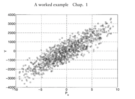
An example of scatter plot (Y vs Ps) obtained with a Monte Carlo experiment of 1000 points is shown in Figure 1.1. Feeding both

Mandyinto a statistical software (SIMLAB included), the analyst

might then try a regression analysis forY. This will return a model of the form

(21)

Figure 1.1 Scatter plot ofYvs.Psfor the model (1.1)Cs =Ct =Cj =300. The scatter plot is made ofN=1000 points.

where the estimates of thebxs are computed by the software based on ordinary least squares. Comparing (1.15) with (1.1) it is easy

to see that if N is at least greater than 3, the number of factors,

thenb0=0,bx=Cx,x=s,t,j.

Normally one does not use thebxcoefficients for sensitivity anal-ysis, as these are dimensioned. The practice is to computes the standardised regression coefficients (SRCs), defined as

βx=bxσx/σy. (1.16)

These provide a regression model in terms of standardised vari-ables

˜

y= y− y¯ σy

; p˜x=

px− p¯x σx

(1.17)

i.e.

˜

y= yˆ− y¯ σy

=

x=s,t,j βx

px− p¯x σx

=

x=s,t,j

βxp˜x (1.18)

where ˆy is the vector of regression model predictions. Equation

(22)

for our portfolio model are equal toCxσx/σy and hence for linear modelsβx= S_xσ because of (1.11). As a result, the values of theβxs can also be read in Table 1.1.

Box 1.2 SIMLAB

You can now try out the relationship βx= Sxσ. If you have

already performed all the steps in Box 1.1, you have to retrieve the saved input and output samples, so that you again reach step 9. Then:

10. On the right most part of the main SIMLAB panel, you activate the SA selection, and select SRC as the sensitivity analysis method.

11. You can now compare the SRC (i.e. theβx) with the values in Table 1.1.

We can now try to generalise the results above as follows: for linear models composed of independent factors, the squared SRCs and Sσ

xs provide the fraction of the variance of the model due to

each factor.

For the standardised regression coefﬁcients, these results can be further extended to the case of non-linear models as follows. The quality of regression can be judged by the model coefﬁcient of determination R2_y. This can be written as

R2_y = N

i=1

( ˆy(i)₋_y_¯₎2

N

i=1

(y(i)₋_y_¯₎2

(1.19)

where ˆy(i)_{is the regression model prediction.}_R2

(23)

variance can be decomposed according to the input factors, leaving us ignorant about the rest, where this rest is related to the non-linear part of the model. In the case of the non-linear model (1.1) we have, obviously, R2

y = 1.

Theβxs are a progress with respect to the Sσx; they can always be computed, also for non-linear models, or for models with no analytic representation (e.g. a computer program that computes

Y). Furthermore the βxs, unlike the Sxσ, offer a measure of sensi-tivity that is multi-dimensionally averaged. WhileSσ

x corresponds

to a variation of factor x, all other factors being held constant,

the βx offers a measure of the effect of factor x that is

aver-aged over a set of possible values of the other factors, e.g. our sample matrix (1.13). This does not make any difference for a linear model, but it does make quite a difference for non-linear models.

Given that it is fairly simple to compute standardised regression coefﬁcients, and that decomposing the variance of the output of interest seems a sensible way of doing the analysis, why don’t we

always use theβxs for our assessment of importance?

The answer is that we cannot, as often R2_y is too small, as e.g. in

the case of non-monotonic models.3

1.2 Modulus version of the simple model

Imagine that the output of interest is no longerY but its absolute value. This would mean, in the context of the example, that we want to study the deviation of our portfolio from risk neutrality. This is an example of a non-monotonic model, where the func-tional relationship between one (or more) input factor and the output is non-monotonic. For this model the SRC-based sensitiv-ity analysis fails (see Box 1.3).

3_{Loosely speaking, the relationship between}_Y_{and an input factor}_X_{is monotonic if the curve}

(24)

Box 1.3 SIMLAB

Let us now estimate the coefﬁcient of determination R2

y for the modulus version of the model.

1. Select ‘Random sampling’ with 1000 executions.

2. Select ‘Internal Model’ and click on the button ‘Open exist-ing conﬁguration’. Select the internal model that you have previously created and click on ‘Modify’.

3. The ‘Internal Model’ editor will appear. Select the formula and click on ‘Modify’. Include the function ‘fabs()’ in the Expression editor. Accept the changes and go back to the main menu.

4. Select ‘Start Monte Carlo’ from the main model panel to generate the sample and execute the model.

5. Repeat the steps in Box 1.2 to see the results. The estimates of SRC appear with a red background as the test of signif-icance is rejected. This means that the estimates are not reliable. The model coefﬁcient of determination is almost null.

Is there a way to salvage our concept of decomposing the

vari-ance of Y into bits corresponding to the input factors, even for

non-monotonic models? In general one has little a priori idea of how well behaved a model is, so that it would be handy to have a more robust variance decomposition strategy that works, what-ever the degree of model non-monotonicity. These strategies are sometimes referred to as ‘model free’.

One such strategy is in fact available, and fairly intuitive to get at. It starts with a simple question. If we could eliminate the

un-certainty in one of the Px, making it into a constant, how much

would this reduce the variance ofY? Beware, for unpleasant

mod-els ﬁxing a factor might actually increase the variance instead of

(25)

The problem could be: how doesVy=σy2change if one can ﬁx

a generic factor Px at its mid-point? This would be measured by

V(Y|Px= p¯x). Note that the variance operator means in this case that while keeping, say, Pj ﬁxed to the value ¯pj we integrate over

Ps,Pt.

V(Y|P¯j = p¯j)= +∞

−∞

+∞

−∞

N( ¯ps, σs)N( ¯pt, σs) [(CsPs+CtPt+Cjp¯j)

−(Csp¯s+Ctp¯t+Cjp¯j)]2dPsdPt. (1.20) In practice, beside the problem already mentioned that

V(Y|Px= p¯x) can be bigger thanVy, there is the practical problem that in most instances one does not know where a factor is best ﬁxed. This value could be the true value, which is unknown at the simulation stage.

It sounds sensible then to average the above measure

V(Y|Px= p¯x) over all possible values ofPx, obtainingE(V(Y|Px)).

Note that for the case, e.g. x= j, we could have written

Ej(Vs,t(Y|Pj)) to make it clear that the average operator is over

Pj and the variance operator is over Ps,Pt. Normally, for a model withkinput factors, one writes E(V(Y|Xj)) with the understand-ing that V is over X−j(a (k−1) dimensional vector of all factors but Xj) and E is over Xj.

E(V(Y|Px)) seems a good measure to use to decide how inﬂu-ential Pxis. The smaller the E(V(Y|Px)), the more inﬂuential the factor Pxis. Textbook algebra tells us that

Vy= E(V(Y|Px))+V(E(Y|Px)) (1.21) i.e. the two operations complement the total unconditional vari-ance. Usually V(E(Y|Px)) is called the main effect of Px on Y, and E(V(Y|Px)) the residual. Given that V(E(Y|Px)) is large if Px is inﬂuential, its ratio to Vy is used as a measure of sensitivity, i.e.

Sx=

V(E(Y|Px))

Vy

(1.22)

(26)

Table 1.2 Sxmeasures for modelYand different values of Cs,Ct,Cj (analytical values).

Cs,Ct,Cj = Cs,Ct,Cj = Cs,Ct,Cj =

Factor 100, 500, 1000 300, 300, 300 500, 400, 100

Ps 0.074 0.762 0.860

Pt 0.463 0.190 0.138

Pj 0.463 0.048 0.002

order effect. It can be always computed, also for models that are not well-behaved, provided that the associate integrals exist. Indeed, if one has the patience to calculate the relative integrals in Equation (1.20) for our portfolio model, one will ﬁnd that Sx= (Sσx)2=βx2,

i.e. there is a one-to-one correspondence between the squared Sσ

x,

the squared standardised regression coefﬁcients and Sx for linear

models with independent inputs. Hence all what we need to do

to obtain the Sxs for the portfolio model (1.1) is to square the

values in Table 1.1 (see Table 1.2). A nice property of theSxs when applied to the portfolio model is that, for whatever combination of Cs,Ct,Cj, the sum of the three indices Ss,St,Sj is one, as one can easily verify (Table 1.2). This is not surprising, as the same was true for theβ_x2when applied to our simple model. Yet the class of models for which this nice property of theSxs holds is much wider (in practice that of theadditive models4_).

Sxis a good model-free sensitivity measure, and it always gives the expected reduction in the variance of the output that one would obtain if one could ﬁx an individual factor.

As mentioned, for a system ofkinput uncertain factors, in

gen-eralk

i=1Si ≤1.

ApplyingSxto model|Y|, modulus ofY, one gets the estimations in Table 1.3. with SIMLAB.

We can see that the estimates of the expected reductions in the

variance of |Y| are much smaller than forY. For example, in the

case of Cs,Ct,Cj =300, ﬁxing Ps gives an expected variance re-duction of 53% for|Y|, whilst the reduction of the variance forY

is 76%.

4_{A model}_Y₌ _f₍_X

1, X2, . . . ,Xk) is additive if fcan be decomposed as a sum ofkfunctions

(27)

Table 1.3 Estimation ofSxs for model|Y|and different values ofCs,Ct,Cj.

Cs,Ct,Cj = Cs,Ct,Cj = Cs,Ct,Cj=

Factor 100, 500, 1000 300, 300, 300 500, 400, 100

Ps 0 0.53 0.69

Pt 0.17 0.03 0.02

Pj 0.17 0 0

Given that the modulus version of the model is non-additive, the sum of the three indices Ss,St,Sj is less than one. For ex-ample, in the case Cs,Ct,Cj =300, the sum is 0.56. What can we say about the remaining variance that is not captured by

the Sxs? Let us answer this question not on the modulus

ver-sion of model (1.1) but – for didactic purposes – on the slightly more complicated a six-factor version of our ﬁnancial portfolio model.

Box 1.4 SIMLAB

Let us test the functioning of a variance-based technique with SIMLAB, by reproducing the results in Table 1.3

1. Select the ‘FAST’ sampling method and then ‘Specify switches’ on the right. Select ‘Classic FAST’ in the combo box ‘Switch for FAST’. Enter something as seed and a num-ber of executions (e.g. 1000). Create a sample ﬁle by giving it a name and selecting a directory.

2. Go back to the left-most part of the SIMLAB main menu and click on ‘Generate’. A FAST-based sample is now avail-able for the simulation.

3. Load the model with the absolute value as in Box 1.3 and click on ‘Start (Monte Carlo)’.

4. Run the SA: a pie chart will appear reporting the estimated

of Sxobtained with FAST. You can also see the tabulated

(28)

Table 1.3 due to sampling error (the sample size is 1000). Try again with larger sample sizes and using the Sobol method, an alternative to the FAST method.

1.3 Six-factor version of the simple model

We now revert to model (1.1) and assume that the quantitiesCxs

are also uncertain. The model (1.1) now has six uncertain inputs. Let us assume

Cs ∼ N(250,200)

Ct ∼ N(400,300)

Cj ∼ N(500,400).

(1.23)

The three distributions have been truncated at percentiles [11, 99.9], [10.0, 99.9] and [10.5, 99.9] respectively to ensure that

Cx> 0.

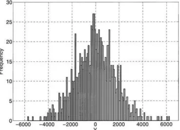
There is no alternative now to a Monte Carlo simulation: the output distribution is in Figure 1.2, and the Sxs, as from Equation (1.22), are in Table 1.4. TheSxs have been estimated using a large

(29)

Table 1.4 Estimates of ﬁrst order effectsSxfor model (1.1) with six input factors.

Factor Sx

Ps 0.36

Pt 0.22

Pj 0.08

Cs 0.00

Ct 0.00

Cj 0.00

Sum 0.66

number of model evaluations (we will come back to this in future chapters; see also Box 1.5).

How is it that all effects forCxare zero? All the Pxare centred

on zero, and hence the conditional expectation value ofY is zero

regardless of the value ofCx, i.e. for model (1.1) we have:

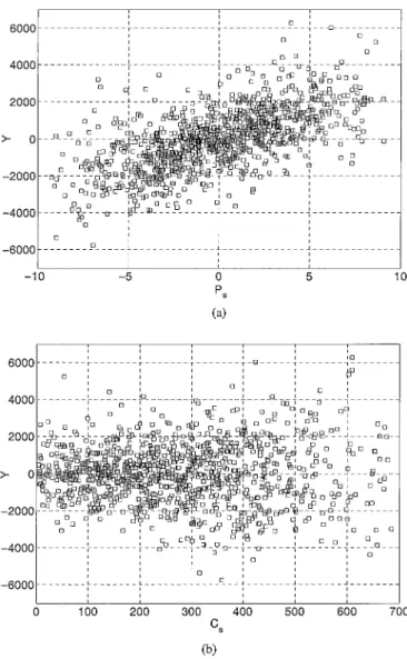
E(Y|Cx=c*x)= E(Y)=0, for allc*x (1.24) and as a result, V(E(Y|Cx))=0. This can also be visualised in

Figure 1.3; inner conditional expectations of Y can be taken

averaging along vertical ‘slices’ of the scatter plot. In the case of

Y vs. Cs (lower panel) it is clear that such averages will form a

perfectly horizontal line on the abscissas, implying a zero variance for the averagedYs and a null sensitivity index. Conversely, forY

vs. Ps(upper panel) the averages along the vertical slices will form an increasing line, implying non-zero variance for the averagedYs and a non-null sensitivity index.

As anticipated the Sxs do not add up to one. Let us now try a

little experiment. Take two factors, say Ps,Pt, and estimate our sensitivity measure on the pair i.e. computeV(E(Y|Ps,Pt))/Vy. By deﬁnition this implies taking the average over all factors except

Ps,Pt, and the variance overPs,Pt. We do this (we will show how later) and call the resultsSc_P_s_P_t, where the reason for the superscript

cwill be clear in a moment. We see that Sc_P_s_P_t =0.58, i.e.

Sc_P_s_P_t = V(E(Y|Ps,Pt))

Vy

(30)

Figure 1.3 Scatter plots for model (1.1): (a) ofYvs.Ps, (b) ofYvs.Cs. The scatter plots are made up of N=1000 points.

This seems a nice result. Let us try the same game withCs,Ps. The results show that now:

S_Cc_s_P_s = V(E(Y|Cs,Ps))

Vy

(31)

Table 1.5 Incomplete list of pair-wise effectsSxzfor model (1.1) with six input factors.

Factors Sxz

Ps,Cs 0.18

Pt,Ct 0.11

Pj,Cj 0.05

Ps,Ct 0.00

Ps,Cj 0.00

Pt,Cs 0.00

Pt,Cj 0.00

Pj,Cs 0.00

Pj,Ct 0.00

Sum of ﬁrst order terms (Table 1.4) 0.66

Grand sum 1

Let us call SCsPs the difference

SCsPs =

V(E(Y|Cs,Ps))

Vy

− V(E(Y|Cs))

Vy

− V(E(Y|Ps))

Vy

= S_Cc_s_P_s −SCs −SPs. (1.27)

Values of this measure for pairs of factors are given in Table 1.5.

Note that we have not listed all effects of the type Px,Py,and

Cx,Cy in this table as they are all null.

Trying to make sense of this result, one might ponder that if the combined effect of two factors, i.e. V(E(Y|Cs,Ps))/Vy, is greater than the sum of the individual effects V(E(Y|Cs))/Vy and

V(E(Y|Ps))/Vy, perhaps this extra variance describes a synergistic or co-operative effect between these two factors. This is in fact the case and SCsPs is called theinteraction (or two-way) effect of

(32)

Tables 1.4–5 that if we sum all ﬁrst-order with all second-order effects we indeed obtain 1, i.e. all the variance of Y is accounted for.

This is clearly only valid for our ﬁnancial portfolio model be-cause it only has interaction effects up to the second order; if we were to compute higher order effects, e.g.

SCsPsPt = S

c

CsPsPt −SCsPs −SPsPt− SCsPt −SCs −SPs −SPt (1.28) they would all be zero, as one may easily realise by inspect-ing Equation (1.1). Sc

CsPsPt on the other hand is non-zero, and is equal to the sum of the three second-order terms (of which only one differs from zero) plus the sum of three ﬁrst-order effects. Speciﬁcally

S_Cc_s_P_s_P_t =0.17+0.02+0.35+0.22=0.76.

The full story for these partial variances is that for a system with

kfactors there may be interaction terms up to the orderk, i.e.

i

Si +

i

j>i

Si j+

i

j>i

l>j

Si jl+. . .S12···k= 1 (1.29)

For the portfolio model with k=6 all terms above the

sec-ond order are zero and only three secsec-ond-order terms are nonzero.

This is lucky, one might remark, because these terms would be a bit too numerous to look at. How many would there be? Six ﬁrst order, 6

2

= 15 second order,6

3

=20 third order, 6

4

=15

fourth order,6 5

=6 ﬁfth order, and one, the last, of orderk=6.

This makes 63, just equal to 2k₋₁₌₂6₋_{1, which is the formula}

to use. This result seems to suggest that the Si, and their higher order relatives Si j, Si jl are nice, informative and model free, but they may become cumbersomely too many for practical use unless the development (1.29) quickly converges to one. Is there a recipe for treating models that do not behave so nicely?

(33)

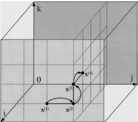
Let us go back to our portfolio model and callX the set of all factors, i.e.

X≡(Cs,Ct,Cj,Ps,Pt,Pj) (1.30) and imagine that we compute:

V(E(Y|X−Cs))

Vy

= V(E(Y|Ct,Cj,Ps,Pt,Pj))

Vy

(1.31)

(the all-but-Csnotation has been used). It should now be apparent that Equation (1.31) includes all terms in the development (1.29), of any order, that do not contain the factorCs. Now what happens if we take the difference

1− V(E(Y|X−Cs))

Vy

? (1.32)

The result is nice; for our model, where only a few higher-order terms are non-zero, it is

1− V(E(Y|X−Cs))

Vy

= SCs +SCsPs (1.33)

i.e. the sum of all non-zero terms that includeCs. The generalisa-tion to a system withkfactors is straightforward:

1− V(E(Y|X−i))

Vy

=sum of all terms of any order

that include the factor Xi.

Note that because of Equation (1.21), 1−V(E(Y|X−i))/Vy =

E(V(Y|X−i))/Vy. We indicate this as STi and call it the total effect term for factor Xi. If we had computed the STi indices for a three-factor model with orthogonal inputs, e.g. our modulus model of Section 1.2, we would have obtained, for example, for factor Ps:

ST Ps = SPs +SPsPt+SPsPj + SPsPtPj (1.34)

and similar formulae for Pt,Pj. For the modulus model, all

terms in (1.34) could be non-zero. Another way of looking at the measures V(E(Y|Xi)), E(V(Y|X−i)) and the corresponding indices Si, STi is in terms of top- and bottom-marginal variances.

(34)

Table 1.6 Estimates of the main effects and total effect indices for model (1.1) with six input factors.

Factor Sx STx

Ps 0.36 0.57

Pt 0.22 0.35

Pj 0.08 0.14

Cs 0.00 0.19

Ct 0.00 0.12

Cj 0.00 0.06

Sum 0.66 1.43

variance that would be left if Xi could be known or could be

ﬁxed. Consequently V(E(Y|Xi)) is the expected reduction in the

output variance that one would get if Xi could be known or

ﬁxed. Michiel J. W. Jansen, a Dutch statistician, calls this latter a top marginal variance. By deﬁnition the total effect measure

E(V(Y|X−i)) is the expected residual output variance that one

would end up with if all factors but Xi could be known or ﬁxed.

Hence the term, still due to Jansen, of bottom marginal variance. For the case of independent input variables, it is always true that

Si ≤ STi, where the equality holds for a purely additive model. In a series of works published since 1993, we have argued that if one can compute all thek Si terms plus all thek STi ones, then one can obtain a fairly complete and parsimonious description of the model in terms of its global sensitivity analysis proper-ties. The estimates for our six-factor portfolio model are given in Table 1.6.

As one might expect, the sum of the ﬁrst-order terms is less than one, the sum of the total order effects is greater than one.

Box 1.5 SIMLAB

(35)

1. Select the ‘FAST’ sampling method and then ‘Specify switches’ on the right. Now select ‘All ﬁrst and total or-der effect calculation (Extended FAST)’ in the combo box ‘Switch for FAST’. Enter an integer number as seed and the cost of the analysis in terms of number of model executions (e.g. 10 000).

2. Go back to the SIMLAB main menu and click on ‘Gen-erate’. After a few moments a sample is available for the simulation.

3. Load the model as in Box 1.3 and click on ‘Start (Monte Carlo)’.

4. Run the SA: two pie charts will appear reporting both the

SxandSTxestimated with the Extended FAST. You can also

look at the tabulated values. Try again using the method of Sobol’.

Here we anticipate that the cost of the analysis leading to Table

1.6 is N(k+2), where the cost is expressed in number of model

evaluations and N is the column dimension of the Monte Carlo

matrix used in the computations, say N=500 to give an order

of magnitude (in Box 1.5 N=1000/8=1250). Computing all

terms in the development (1.29) is more expensive, and often pro-hibitively so.5We would also anticipate, this time from Chapter 4,

that a gross estimate of the STxterms can be obtained at a lower

cost using an extended version of the method of Morris. Also for this method the size is proportional to the number of factors.

1.4 The simple model ‘by groups’

Is there a way to compact the results of the analysis further? One might wonder if one can get some information about the overall sensitivity pattern of our portfolio model at a lower price. In fact a nice property of the variance-based methods is that the variance

(36)

Table 1.7 Estimates of main effects and total effect indices of two groups of factors of model (1.1).

Factor Sx STx

P≡(Ps,Pt,Pj) 0.66 1.00

C≡(Cs,Ct,Cj) 0.00 0.34

Sum 0.66 1.34

decomposition (1.29) can be written for sets of factors as well. In our model, for instance, it would be fairly natural to write a variance decomposition as:

SC+SP+SC,P=1 (1.35)

whereC= Cs,Ct,Cj andP= Ps,Pt,Pj. The information we ob-tain in this way is clearly less than that provided by the table with all Si and STi.6

Looking at Table 1.7 we again see that the effect of theCset at the ﬁrst order is zero, while the second-order term SC,Pis 0.34, so

it is not surprising that the sum of the total effects is 1.34 (the 0.34 is counted twice):

STC= SC+SC,P

STP = SP+SC,P (1.36)

Now all that we know is the combined effect of all the amounts of hedges purchased,Cx, the combined effect of all the hedged

port-folios, Px, plus the interaction term between the two. Computing

all terms in Equation 1.35 (Table 1.7) only costs N×3, one set of

sizeN to compute the unconditional mean and variance, one forC

and one forP,SC,Pbeing computed by difference using (1.35). This

is less than the N×(6+2) that one would have needed to

com-pute all terms in Table 1.6. So there is less information at less cost, although cost might not be the only factor leading one to decide to present the results of a sensitivity analysis by groups. For instance, we could have shown the results from the portfolio model as

Ss+St+Sj+Ss,t+St,j+Ss,j+Ss,t,j =1 (1.37)

6_{The ﬁrst-order sensitivity index of a group of factors is equivalent to the closed effect of all}

(37)

Table 1.8 Main effects and total effect indices of three groups of factors of model (1.1).

Factor Sx STx

s≡(Cs,Ps) 0.54 0.54

t≡(Ct,Pt) 0.33 0.33

j≡(Cj,Pj) 0.13 0.13

Sum 1 1

wheres≡(Cs,Ps) and so on for each sub-portfolio item, where a sub-portfolio is represented by a certain amount of a given type of hedge. This time the problem has become additive, i.e. all terms of second and third order in (1.37) are zero. Given that the interac-tions are ‘within’ the groups of factors, the sum of the ﬁrst-order effects for the groups is one, i.e. Ss+St+Sj= 1, and the total

indices are the same as the main effect indices (Table 1.8).

Different ways of grouping the factors might give different in-sights into the owner of the problem.

Box 1.6 SIMLAB

Let us estimate the indices in Table 1.7 with SIMLAB.

1. Select the ‘FAST’ sampling method and then ‘Specify switches’ on the right. Now select ‘All ﬁrst and total or-der effect calculation on groups’ in the combo box ‘Switch for FAST’. Enter something as seed and a number of exe-cutions (e.g. 10 000).

2. Instead of generating the sample now, load the model ﬁrst by clicking on ‘Conﬁgure (Monte Carlo)’ and then ‘Select Model’.

3. Now click on ‘Start (Monte Carlo)’. SIMLAB will generate the sample and run the model all together.

4. Run the SA: two pie charts will appear showing both the

SxandSTxestimated for the groups in Table 1.7. You can

(38)

1.5 The (less) simple correlated-input model

We have now reached a crucial point in our presentation. We have to abandon the last nicety of the portfolio model: the orthogonality (independence) of its input factors.7

We do this with little enthusiasm because the case of dependent factors introduces the following considerable complications.

1. Development (1.29) no longer holds, nor can any higher-order term be decomposed into terms of lower dimensionality, i.e. it is no longer true that

V(E(Y|Cs,Ps))

Vy

= S_Cc_s_P_s = SCs +SPs +SCsPs (1.38)

although the left-hand side of this equation can be computed, as we shall show. This also impacts on our capacity to treat factors into sets, unless the non-zero correlations stay conﬁned within sets, and not across them.

2. The computational cost increases considerably, as the Monte Carlo tricks used for non-orthogonal input are not as efﬁcient as those for the orthogonal one.

Assume a non-diagonal covariance structureC for our problem:

C =

Ps Pt Pj Cs Ct Cj

Ps 1

Pt 0.3 1

Pj 0.3 0.3 1

Cs . . . 1

Ct . . . −0.3 1

Cj . . . −0.3 −0.3 1

(1.39)

We assume the hedges to be positively correlated among one an-other, as each hedge depends upon the behaviour of a given stock

7_{The most intuitive type of dependency among input factors is given by correlation. However,}

(39)

Table 1.9 Estimated main effects and total effect indices for model (1.1) with correlated inputs (six factors).

Factor Sx STx

Ps 0.58 0.35

Pt 0.48 0.21

Pj 0.36 0.085

Cs 0.01 0.075

Ct 0.00 0.045

Cj 0.00 0.02

Sum 1.44 0.785

price and we expect the market price dynamics of different stocks to be positively correlated. Furthermore, we made the assumption that theCxs are negatively correlated, i.e. when purchasing more of a given hedge investors tends to reduce their expenditure on another item.

The marginal distributions are still given by (1.2), (1.23) above. The main effect coefﬁcients are given in Table 1.9. We have also estimated the STxindices as, for example, for Ps:

ST Ps =

E(V(Y|X−Ps))

V(Y) =1−

V(E(Y|X−Ps))

V(Y) (1.40)

with a brute force method at large sample size. The calculation of total indices for correlated input is not implemented in SIMLAB.

(40)

Table 1.10 Decomposition ofV(Y) and relative value ofV(E(Y|Xi)), E(V(Y|X−i)) for two cases: (1) orthogonal input, all models and (2) non-orthogonal input, additive models. When the input is non-orthogonal and the model non-additive,V(E(Y|Xi)) can be higher or lower than E(V(Y|X−i)).

Case (1) Orthogonal input factors, all models. For additive models the two rows are equal.

V(E(Y|Xi)) top marginal. (or main effect) of Xi

E(V(Y|Xi)) bottom marginal. (or total effect) ofX−i

E(V(Y|X−i)) bottom marginal (or total effect) ofXi

V(E(Y|X−i)) top marginal (or main effect) ofX−i

Case (2) Non-orthogonal input factors, additive models only. If the dependency between inputs vanishes, the two rows become equal. For the case whereXi andX−iare perfectly correlated both theE(V(Y|.)) disappear and both theV(E(Y|.)) become equal toV(Y).

V(E(Y|Xi)) top marginal ofXi

E(V(Y|X−i)) bottom marginal ofXi

E(V(Y|Xi)) bottom marginal ofX−i V(E(Y|X−i)) top

marginal ofX−i

V(Y) (Unconditional)

input factors it will be STi ≤Si. In the absence of interactions

(additive model) it will be STi = Si for the orthogonal case. If,

still with an additive model, we now start imposing a depen-dency among the input factors (e.g. adding a correlation struc-ture), then STi will start decreasing as E(V(Y|X−i)) will be lower because having conditioned on X−i also limits the variation of Xi (Table 1.10).

We take factor Ps as an example for the discussion that follows.

Given that for the correlated input case ST Ps can no longer be

(41)

to determine if the inﬂuence of Ps is zero. If Ps is totally non-inﬂuential, then surely

E(V(Y|X−Ps))=0 (1.41)

because ﬁxing ‘all but Ps’ results in the inner variance over Ps

being zero (under that hypothesis the variance ofY is driven only

by non-Ps), and this remains zero if we take the average over all possible values of non-Ps. As a result,ST Psis zero ifPsis totally non-influential. It is easy to see that the condition E(V(Y|X−P_s)) =0 is necessary and sufficient for factorPsto be non-influent, under any model or correlation/dependency structure among input factors.

1.6 Conclusions

This ends our analysis of the model in Equation (1.1). Although we haven’t given the reader any of the computational strategies to compute the Sx, STxmeasures, it is easy to understand how these can be computed in principle. After all, a variance is an integral. It should be clear that under the assumptions that:

1. the model is not so terribly expensive that one cannot afford Monte Carlo simulations, and

2. one has a scalar objective function Y and is happy with its

variance being the descriptor of interest.

Then

1. variance based measures offer a coherent strategy for the

de-composition of the variance ofY;

2. the strategy is agile in that the owner of the problem can decide if and how to group the factors for the analysis;

3. this strategy is model free, i.e. it also works for nasty,

non-monotonic, non-additive models Y, and converge to

(42)

4. it remains meaningful for the case where the input factors are non-orthogonal;

(43)

(44)

2

ANALYSIS FOR IMPORTANCE

ASSESSMENT

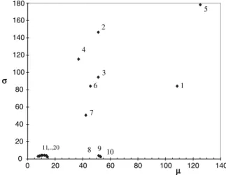
In this chapter we introduce some examples, most of which will later serve as test cases. The examples are described in detail in Chapter 3. Here a ﬂash description is offered, for the purpose to illustrate different problem settings for SA. The hurried reader can use these descriptions to match the example with their own application. Next, a deﬁnition of sensitivity analysis is offered, complemented by a discussion of the desirable properties that a sensitivity analysis method should have. The chapter ends with a categorisation (a taxonomy) of application settings, that will help us to tackle the applications effectively and unambiguously.

2.1 Examples at a glance

Bungee jumping

We are physicist and decide to join a bungee-jumping club, but

want to model the system ﬁrst. The asphalt is at a distanceH(not

well quantiﬁed) from the launch platform. Our mass M is also

uncertain and the challenge is to choose the best bungee cord (σ = number of strands) that will allow us to almost touch the ground below, thus giving us real excitement. We do not want to use cords that give you a short (and not exciting) ride. So, we choose the minimum distance to the asphalt during the oscillation (hmin) as a

convenient indicator of excitement. This indicator is a function of

three variables:H, Mandσ.

Our ﬁnal target is to identify the best combination of the three variables that gives as the minimum value ofhmin(though this must

(45)

−10

−5 0 5 10 15 20 25 30 35 40

0 20 40 60 80 100

h mi

n

(m

)

Frequency of events

Asphalt Surface

Figure 2.1 Uncertainty analysis of the bungee-jumping excitement indica-torhmin.

remain positive!). This search is a simple minimisation problem with constraints, which can be managed with standard optimisa-tion techniques. However, the uncertanity in the three variables implies an uncertinity onhmin. If such uncertainty is too wide, the

risk of a failure in the jump is high and must be reduced. Under these circumstances, it is wise to investigate, through sensitivity

analysis, which variable drives most of the uncertainty on hmin.

This indicates where one should improve our knowledge in order to reduce the risk of failure.

The uncertainty analysis (Figure 2.1), shows the uncertainty on

hmin due to the uncertainties in H, M and σ (more details will

be given in Chapter 3). The probability of a successful jump is 97.4%. The sensitivity analysis (Chapter 5) shows that the num-ber of strands in the cord is the risk-governing variable, worth examining in more detail. Meanwhile, we should not waste time

improving the knowledge of our massM, as its effect on the

(46)

Figure 2.2 Monte Carlo based uncertainty analysis of Y= Log (PI (Incineration)/PI(Landﬁll)) obtained by propagating the uncertainty of waste inventories, emission factors, weights for the indicators etc. The uncertainty distribution is bimodal, with one maximum for each for the two waste man-agement alternatives, making the issue non-decidable.

Decision analysis

A model is used to decide whether solid waste should be burned or disposed of in landﬁll, in an analysis based on Austrian data for 1994. This is a methodological exercise, described in detail in

Saltelli et al. (2000a, p. 385). An hypothetical Austrian decision

maker must take a decision on the issue, based on an analysis of the environmental impact of the available options, i.e. landﬁll or incineration. The model reads a set of input data (e.g. waste inven-tories, emission factors for various compounds) and generates for each option a pressure-to-decision index PI. PI(I) quantiﬁes how much the option (I) would impact on the environment. The model

output is a function, Y, of the PIs for incineration and landﬁll,

built in such a way as to suggest incineration for negative values

of Y and landﬁll otherwise. Because most of the input factors to

the analysis are uncertain, a Monte Carlo analysis is performed, propagating uncertainties to produce a distribution of values for

Y (Figure 2.2). What makes this example instructive is that one of

(47)

3

16

58

9

5 5 ₄

0 10 20 30 40 50 60 70

Tu Data E/F GWP W_E EEC STH

% of V(Y) accounted for by each input factor

Figure 2.3 Variance-based decomposition of the output variable Y. The in-put factors (and their cardinality) are: E/F(1): trigger factor used to select randomly, with a uniform discrete distribution, between the Finnish and the Eurostat sets of indicators; TU (1), Territorial Unit: trigger that selects be-tween two spatial levels of aggregation for input data; DATA (176), made up of activity rates (120), plus emission factors (37) plus National emissions (19); GWP (1), weight for greenhouse indicator (in the Finnish set): three time-horizons are possible: W E (11), Weights for Eurostat indicators; EEC (1), approach for Evaluating Environmental Concerns: Target values (Adri-aanse 1993) or expert judgement (Puolamaa et al., 1996) and STH (1) is a single factor that selects one class of Finnish stakeholders from a set of eight possible classes. The factor E/F triggering the choice of the system of indicators accounts for 58% of the variance ofY.

(48)

Figure 2.4 Smirnov test statistics (see Box 2.1 Smirnov) for the two cumu-lative sub-sample distributions obtained splitting the sample of each input factor according to the sign of the outputY. An unequivocal split between the solid and the dotted curves can be observed when the E/F input factor is plotted on thex-axis. When the GWP factor is plotted on thex-axis, the split between the two curves is less signiﬁcant.

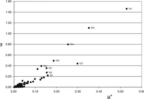
A model of ﬁsh population dynamics

A stage-based model was developed by Zald´ıvar et al. (1998) to

(49)

current off western North America and the Benguela current off south-western Africa. Comparing geological data and simulation results, Zaldivaret al. showed that although environmental fluctu-ations can explain the magnitude of observed varifluctu-ations in geolog-ical recordings and catch data of pelagic fishes, they cannot explain the low observed frequencies. This implies that relevant non-linear biological mechanisms must be included when modelling fish pop-ulation dynamics.

Despite the fact that the ecological structure of the model has been kept as simple as possible, in its ﬁnal version the model con-tains over 100 biologically and physically uncertain input factors. With such a large number of factors, a sensitivity screening exer-cise may be useful to assess the relative importance of the various factors and the physical processes involved. The sensitivity method

proposed by Morris (1991) and extended by Campolongo et al.

(2003b) has been applied to the model. The model output of in-terest is the annual population growth. The experiment led to a number of conclusions as follows.

r

The model parameters describing the population of sardines

are not identified as substantially influential on the population growth. This leads to the question: ‘Is this result reflecting a truly smaller role of this species with respect to the others or is it the model that should be revised because it does not properly reflect what occurs in nature?’

r

A second conclusion is that the model parameters describing the

inter-specific competition are not very relevant. This calls for a possible model simplification; there is no need to deal with a 100-factors model that includes inter-specific competitions when, to satisfy our objective, a lower level of complexity and a more viable model can be sufficient.

r

Finally, a subset of factors that have the greatest effect on

(50)

The risk of a ﬁnancial portfolio

Imagine that a bank owns a simple ﬁnancial portfolio and wants to assess the risk incurred in holding it. The risk associated with the portfolio is deﬁned as the difference between the value of the portfolio at maturity, when the portfolio is liquidated, and what it would have gained by investing the initial value of the portfolio at the market free rate, rather than putting it in the portfolio. The model used to evaluate the portfolio at each time is based on the assumption that the spot interest rate evolves on the market according to the Hull and White one-factor stochastic model (see details in Chapter 3).