www.scielo.br/cam
Steam injection into water-saturated porous rock
J. BRUINING1, D. MARCHESIN2 and C.J. VAN DUIJN3
1Dietz Laboratory, Centre of Technical Geoscience, Mijnbouwstraat 120 2628 RX Delft, The Netherlands
E-mail: [email protected]
2Instituto Nacional de Matemática Pura e Aplicada, Estrada Dona Castorina 110 22460-320 Rio de Janeiro, RJ, Brazil
E-mail: [email protected]
3Technische Universiteit Eindhoven, Den Dolech 2 5600 MB Eindhoven, The Netherlands
E-mail: [email protected]
Abstract. We formulate conservation laws governing steam injection in a linear porous medium containing water. Heat losses to the outside are neglected.
We find a complete and systematic description of all solutions of the Riemann problem for the injection of a mixture of steam and water into a water-saturated porous medium. For ambient pressure, there are three kinds of solutions, depending on injection and reservoir conditions. We show that the solution is unique for each initial data.
Mathematical subject classification:76S05, 35L60, 35L67. Key words:porous medium, steamflood, travelling waves, multiphase flow.
Introduction
Steam injection is an effective technique to restore groundwater aquifers contam-inated with non-aqueous phase liquids (NAPL’s) such as hydrocarbon fuels and halogenated hydrocarbons [15]. It is also one of the most effective methods to
#558/02. Received: 28/XII/02. Accepted: 18/VIII/03.
recover oil from medium to heavy oil reservoirs [13]. The main feature of steam injection is the steam condensation front (SCF), which marks the boundary be-tween the upstream zone at boiling temperature and the downstream liquid zone below the boiling temperature. Depending on the situation there may exist an isothermal steam-water shock at the boiling temperature (H I SW) instead of the
SCF. The main result of this work is a complete and systematic classification of the structure of all possible cases of Riemann solutions. As a first step we have ignored the presence of NAPL’s in our model. The model has also appli-cations outside the use of steam for oil recovery or pollutant product recovery, for example in chemical engineering.
There is an extensive literature on models of steam drive. Their main focus is the internal structure of the steam condensation front and they are reviewed in [4], [5].
In this article we limit ourselves to the simple case of steam displacing water. Our aim is to investigate a unique well posed solution of the Riemann problem for all possible values of the model parameters, providing mathematical validation of our model. This is the first step towards solving the full problem of groundwater NAPL removal.
In Section 1, the physical model is presented. It is described mathematically by balance equations of mass and thermal energy, which are rewritten into a form suitable for analysis.
Section 2 presents the basic waves arising in the model; the main concern is to identify their speeds, so as to be able to find the order in which they may appear in a linear steam injection experiment. In Section 3, we see that for certain values of initial and boundary data, some of these speeds coincide, giving rise to bifurcation and structural change in the Riemann solution. All solutions of the Riemann problem are in Section 4. Section 5 verifies that theSCF satisfies Lax’s shock inequalities, but not strictly. Section 6 summarizes our results and conclusions.
1 Physical and mathematical model
1.1 Physical model
We consider linear steam displacement in a homogeneous reservoir of constant permeability and porosity. The reservoir is initially saturated with water. The pressure gradients∂pw/∂x,∂pg/∂xdriving the fluids are small with respect to the prevailing system pressurepdivided by the length of the reservoir. In partic-ular, within the short steam condensation zone pressure variations are negligible. Hence we disregard the effect of pressure variation on the density of the fluids and on their thermodynamic properties. The reservoir is horizontal, so gravitational effects vanish.
A steam-water mixture is injected at constant rateuinjand constant steam/water injection ratio. Transverse heat losses are disregarded. We neglect capillary forces after steam breakthrough at the production end of the reservoir to avoid problems with the capillary end effect, which is outside the present scope of our interest.
The effects of temperature on the fluid properties,e.g. water viscosity µw, steam viscosityµg, water densityρwand steam densityρgare taken into account. Darcy’s Law determines the fluid motion. The temperature dependence of heat capacities and of the evaporation heat are also taken into account. Capillary pressure as well as an effective longitudinal heatconductionterm are included.
We have chosen to describe condensation in terms of a steam mass conden-sation rate equation. The mass condenconden-sation rateqis always positive when the temperature drops below the boiling temperatureTbas long as not all steam has condensed, that isSw <1.
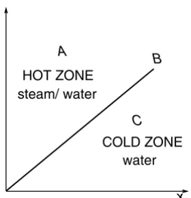
rate is increased further a zone in which the steam saturation is constant will develop preceding the rarefaction wave until the steam saturation in the hot zone is constant. After this constant state there is aSCF and a cold water region. This will be called situationII. Finally when the water–steam injection ratio is increased further, the steam bank will not be fast enough to reach the cooling front separating the hot and cold water zones; thus there is noSCF. This and higher ratios originate in situationIII. In all regimes, there is a hot zone and a cool zone, whose boundary moves with constant speed, as shown in Fig. 1.
t
x
steam/ water
water
A
B
C
HOT ZONE
COLD ZONE
Figure 1 –B: Condensation front or cooling front.
Each of the enthalpies per unit volume Hw(T ), Hr(T ), Hg(T ) ([J /m3
]) is defined with respect to the enthalpy at the initial reservoir temperatureT0at the standard state. This means that they are all zero at the initial temperatureT0.
The enthalpy of steam is subdivided in a sensible partHs
g(T )and a latent part Hgl(T0),i.e. Hg(T ) = Hgs(T )+Hgl(T0). The sensible heatHgs(T0)is zero at
the initial reservoir temperature. The evaporation heat or the latent heat per unit mass at the initial reservoir temperatureT0is denoted by
We assume Darcy’s law for two-phase flow, water and steam respectively, without gravity terms:
uw = −kkrw
µw ∂pw
∂x , ug= − kkrg
µg ∂pg
∂x . (2)
The liquid water viscosity and the steam viscosity are temperature-dependent functions (see Appendix A).
As discussed in [4], the water mass source term is taken as
q =
qb(T −Tb)(Sw−1) for T ≤Tb, 0≤Sw ≤1;
0 otherwise.
(3)
This term is motivated by the idea that the condensation rate is determined by a ‘‘driving force’’ which is proportional to its departure from equilibriumSw =1 andT =Tb( see also reference [11]). The value ofqbis considered very large.
1.2 The model equations
The mass balance equation of liquid water and steam read as follows:
∂(ϕρwSw)
∂t +
∂(ρwuw)
∂x = q, (4)
∂(ϕρgSg)
∂t +
∂(ρgug)
∂x = −q. (5)
The rock porosityϕis assumed to be constant. We include longitudinal heat conduction, but neglect heat losses to the surrounding rock, in the energy balance equation given below. By our assumption of almost constant pressure we ignore adiabatic compression and decompression effects. Thus the energy balance is (See reference [2], Table 10.4-1):
∂ ∂t
Hr+ϕSwHw+ϕSgHg+ ∂
∂x
uwHw+ugHg= ∂
∂x
κ∂T ∂x
. (6)
Hereκ is the composite conductivity of the rock–fluid system [1]:
κ =κr +ϕSwκw+Sgκg. (7)
Equations (4) and (5) are combined with the heat balance equation (6), where we also use separation in sensible and latent quantities, to obtain:
∂ ∂t
Hr +ϕSwHw+ϕSgHgs
+ ∂
∂x
uwHw+ugHgs
− ∂ ∂x κ∂T ∂x = −∂ ∂t
ϕSgHgl
− ∂
∂x
ugHgl
= −∂
∂t
ϕSgρg0− ∂
∂x
ugρg0
= −0
∂ ∂t
ϕSgρg+ ∂
∂x
ugρg
.
Using Eq. (5), this yields
∂ ∂t
Hr +ϕSwHw+ϕSgHgs + ∂
∂x
uwHw+ugHgs
=q0+ ∂
∂x κ∂T ∂x . (8)
Let us define the fractional flow functions for water and steam:
fw = krw/µw
krw/µw +krg/µg, fg =
krg/µg
krw/µw+krg/µg. (9)
The capillary pressure
Pc =Pc(Sw)=pg−pw (10)
which is given by Equation (83), is a strictly monotone decreasing function; it appears in the definition of the capillary diffusion coefficient:
= −fwkkrg µg
dPc
dSw ≥0. (11)
We notice thatvanishes precisely at water saturationsSw =SwcandSw =1. Using Darcy’s law (2) (in the absence of gravitational effects) and the definition ofPcgiven in Eq. 10, one can easily show from Eqs. (2) and (11) that:
uw =ufw−∂Sw
∂x , ug=ufg− ∂Sg
∂x , (12)
where
is the total or Darcy velocity and acts as a saturation-dependent capillary diffusion coefficient.
Substituting (12) into Equations (4), (5) and (8) leads to
ϕ∂ (ρwSw)
∂t +
∂ (ρwufw)
∂x =q+
∂ ∂x ρw∂Sw ∂x , (14) ϕ∂ ρgSg ∂t +
∂ρgufg
∂x = −q+ ∂ ∂x ρg∂Sg ∂x , (15) ∂ ∂t
Hr +ϕHwSw+ϕHgsSg + ∂
∂x
u
Hwfw+Hgsfg
=q0+ ∂
∂x
Hw−Hgs∂Sw ∂x + ∂ ∂x κ∂T ∂x . (16)
The governing system of equations is (14)–(16).
As to initial conditions, we assume that the reservoir is filled with water at saturationSw(x, t =0)=S0
w =1 with constant temperatureT (x, t =0)=T0.
As to boundary conditions, the total injection rateuinj is specified and constant (see Appendix A). The constant steam-water injection ratio is specified in terms of the water saturationSwinj at the injection side.
Lemma 1. In a region where the temperature is constant (and noncritical),
q=0.
Proof. If the temperature is constant, the enthalpies are constant, so Eq. (8) becomes
ϕHw∂Sw ∂t +ϕH
s g
∂Sg ∂t +Hw
∂uw ∂x +H
s g
∂ug ∂x =q
0. (17)
We regroup Eq. (17) and use the mass balance equations (4) and (5). Since the temperature is constant the densities are constant too, so Eq. (17) becomes
Hw ϕ∂Sw ∂t + ∂uw ∂x +Hgs
ϕ∂Sg ∂t + ∂ug ∂x
= q0, Hw
ρwq− Hs
g
ρgq =q 0, Hw ρw − Hs g ρg − 0
q = 0.
The term in parenthesis in Eq. (18) is minus the enthalpy per unit mass required to convert water into steam and is therefore non-zero. Consequently we must have thatq =0. Summarizing, we can say that if the temperature is constant in
space and time then there is no source term.
Remark 1. It is easy to see that the source termq vanishes in regions where either (i) the temperature is constant, (ii) the gas saturation is zero, (iii) the water saturation is zero.
2 The hyperbolic framework
By ignoring capillary pressure and heat conduction diffusive effects, we are in the framework of first order hyperbolic conservation laws; this framework is useful to study the basic waves of the model. Throughout this section we assume that all fluids are in thermodynamic equilibrium. Equations (14) and (15), the mass balance equation of liquid water and steam combined with Darcy’s law read as follows:
∂(ϕρwSw)
∂t +
∂(ρwufw)
∂x = q, (19)
∂(ϕρgSg)
∂t +
∂(ρgufg)
∂x = −q. (20)
When we add these equations, we obtain the total water conservation:
ϕ ∂ ∂t
ρwSw+ρgSg+ ∂
∂x
u(ρwfw+ρgfg)
=0. (21)
Eq. (16) becomes
∂ ∂t
Hr +ϕHwSw+ϕHgsSg
+ ∂
∂x
u(Hwfw+Hgsfg)
=q0, (22) or equivalently, as in Eq. (6)
∂ ∂t
Hr +ϕHwSw+ϕHgSg+ ∂
∂x
u(Hwfw +Hgfg)
=0. (23)
Remark 2. Notice that all speeds defined by Equations (21) and (22) are proportional tou. Thus we can choose any speed to parameterize all the other ones.
Let us consider all regions where the mass transfer term vanishes. The mass transfer can vanish because of several reasons. Based on these reasons, we classify the regions in the following table. Because the mass source term vanishes (Eq. (3)), we have the following zones in the reservoir:
Sw\T T =Tb T < Tb Sw <1 hot steam zone xxxxxxxxxxxxx
Sw =1 hot water zone cold water zone
Table 1 – Classification according to mass source term.
We call ‘‘hot steam-water region’’, or ‘‘hot region’’, the hot steam zone to-gether with hot water zone, whereT =Tb. We call ‘‘liquid water region’’ the hot water zone together with the cold water zone.
These regions overlap on the hot water zone.
Remark 3. There is no ‘‘cold steam zone’’ in Table 1 because at thermody-namical equilibrium steam cannot exist at a temperature lower thanTb.
As we will see, a configuration composed by sequential zones of hot steam, hot water and cold water is possible, counting away from the injection point. At the first interfaceSw =1 is reached, while at the second oneT =T0is reached. A configuration containing only the hot steam zone and the cold water zone is possible if we interpose the so calledSCF, where both saturation and temperature change abruptly.
2.1 The hot region
This region starts with the hot steam zone, where steam is injected at boiling temperature Tb. We claim that the Darcy velocity u (given by Eq. (13)) in
the hot region is independent of position. To prove this fact we use equations (19), (20). As the temperature isTb, the source term (such as given in Eq. (3))
vanishes and the densities are constant. We can divide Eqs. (19), (20) by the densities and add the resulting equations and obtain our claim.
Since the Darcy velocityuis a constant in space in the hot region and since in this work we also take thatuinj is constant in time, the temperatureTband the Darcy velocityubare constant in this region. Thus Eq. (22) is satisfied trivially,
and both Eqs. (19) and (20) reduce to any of the two equivalent forms of the Buckley-Leverett problem for steam and water that follows:
ϕ∂Sw ∂t +u
b∂fw
∂x =0, ϕ ∂Sg
∂t +u b∂fg
∂x =0. (24)
This equation governs propagation in the hot steam zone, as long as steam and water are both present. The classical Ole˘ınik construction [10], or equivalently, the fractional flow theory [12] describe waves in this zone.
We will denote byvb
s the speed of propagation of saturation waves in the hot
steam zone. It is obtained from Eq. (24) as the characteristic speed:
vsb=vsb(Sw;ub)= u
b
ϕ ∂fwb
∂Sw(Sw), (25)
whereT =Tband we use the nomenclaturefb
w(Sw)=fw(Sw, Tb).
A particular Buckley-Leverett shock for (24) turns out to play a relevant role, separating a mixture of steam and water from pure water, both at boiling temper-ature. We call it thehot isothermal steam-water shockorH I SW shock between the(−)state(Swb, Tb, ub)containing steam and the (+)state(1, Tb, ub) con-taining water at boiling temperature. It has speedvb
g,w given by
vg,wb =vbg,w(Swb;ub)= u
b
ϕ
fgb(Sgb)
Sb g
= u
b
ϕ
1−fwb(Swb)
1−Sb w
. (26)
saturation given in Eq. (82), withng=2 we obtain:
vg,wb (Sw =1;u b
)=0. (27)
Similarly, forSb
w ≤Swcfrom Eqs. (82) and (9),
vbg,w = u
b
ϕ(1−Sb w)
>0. (28)
Remark 4. It is easy to verify thatvb
s in Eq. (25) is monotonously increasing
inSwb whenSwbis less thanSinf l, the inflection abscissa offw, and monotonously decreasing whenSb
wis larger thanSinf l.
2.2 Liquid water region
We recall that the liquid water zone consists of the hot region, which is also part of the hot region examined in Section 2.1, and of the cold water zone.
In the liquid water zone there is no steam, so there is no mass transfer between steam and water. Soq =0. Also, in the liquid regionSw =1, so Eqs. (21) and (22) reduce to
ϕ∂ρw ∂t +
∂(uρw)
∂x = 0, (29)
∂ ∂t
Hr +ϕHw+∂(uHw)
∂x =0. (30)
2.2.1 Cooling contact discontinuity
We will assume that ρw and Cwp are essentially constant in the pressure and temperature region of interest. A more complete discussion can be found in [5].
Let us consider a temperature discontinuity fromTbtoT0, with speedvb,0 w in
the liquid water between the hot left (or upstream) state(Sw =1, T =Tb, ub)
and the cold right (or downstream) state (Sw = 1, T = T0, u0). For such
a cooling contact discontinuity, from Eqs. (29) and (30) one can obtain the following Rankine-Hugoniot relation, where we denote byubandu0the Darcy
velocities at the discontinuity sides corresponding toTbandT0:
vwb,0 = u
0ρ0
w−ubρwb ϕ(ρ0
w−ρwb)
= u
0H0
w−ubHwb (H0
r +ϕHw0)−(Hrb+ϕHwb)
where
Hwb =Hw(Tb), Hrb=Hr(Tb), ρwb =ρw(Tb). (32)
We recall that our convention is that enthalpies vanish atT0; then the Rankine-Hugoniot condition can be rewritten as
vwb,0= u
0ρ0
w−ubρwb ϕ(ρ0
w−ρwb)
=ub H
b w Hb
r +ϕHwb
. (33)
From the second equality in Eq. (33), we obtain that
ub= H
b r +ϕH
b w Hb
rρwb/ρw0 +ϕHwb
u0, (34)
which expresses the conservation of water mass. From the last term in Eq. (33) and from Eq. (34):
vb,0w = H
b w Hb
rρwb/ρw0 +ϕHwb
u0. (35)
Remark 5. Notice that the dependence ofρw on temperature is often small. Ifρw were independent of temperature (constant), then Eq. (34) would imply thatub=u0.
Remark 6. Since all speeds in this problem scale withu, anduinj is constant
in time,u0andubare constant in time.
Remark 7. In the hot water zone, bothSw =1 andT =Tb, soq
=0. Since the temperature is constant, so isρw, thus Eq. (29) says that u is a constant, which has already been called ub in Section 2.1. Equation (30) says that the characteristic speed (of temperature waves) in the hot water zone is
vwb = C
p w(Tb) Crp(Tb)+ϕCw(Tp b)
ub. (36)
This is the propagation speed of small temperature perturbations nearT =Tb
Remark 8. Under the assumptions thatρwandCwpare constant in pressure and temperature, the characteristic speeds (36) evaluated atTb, and evaluated atT0
coincide with the discontinuity speed (31). In gas dynamics, discontinuities with this coincidence property are called contact discontinuities. Hence the name we gave to this wave.
2.3 Steam condensation front
This is a discontinuity joining a state(−)containing steam and water at temper-atureTbto pure water at temperatureT0, a state(+); that is, it separates the hot steam zone from the cold water zone. It satisfies the following Rankine-Hugoniot conditions with speedvSCF for Eqs. (21), (23) between states(Sb
w, Tb, ub)and (Sw0 =1, T0, u0). From the water balance (21) we obtain:
ubρwfw+fgρg−−ϕvSCFρwSw+Sgρg−
=u0ρwfw+fgρg+−ϕvSCF ρwSw+Sgρg+ (37)
and from the energy balance (23) we obtain:
ub
Hwfw+Hgfg−
−vSCF
Hr +ϕHwSw+ϕHgSg−
=u0
Hwfw+Hgfg+
−vSCF
Hr+ϕHwSg+ϕHgSg+
. (38)
As no steam exists on the right of theSCF, we can say thatSw0 =fw0=1 and
S0
g =fg0=0 and thus Eq. (37) becomes
ubρwfw+ρgfg−−ϕvSCFρwSw+ρgSg−=ρ0w
u0−ϕvSCF. (39) Under the same conditions we obtain for the heat balance equation (38):
ubHwfw+Hgfg−−vSCF Hr +ϕHwSw+ϕHgSg−
=u0Hw0−v SCF
Hr0+ϕH 0 w
=0. (40)
velocity it follows from Eqs. (39), (40) that
u0=ub
ρgb
ρ0 w
fgb+ρ
b w ρ0 w
fwb −ϕvSCF
ρgb
ρ0 w
Sgb+ρ
b w ρ0 w
Swb −1 , (41)
vSCF =ub H b wf
b w+H
B g f
b g Hb
r +ϕHwbSwb +ϕHgBSgb
, (42)
where we used the nomenclature that follows from Eq. (1):
HgB ≡Hg(Tb)=Hgs(Tb)+Hgl =Hgb+0ρg0. (43) BecauseSb
g =1−Swb,fgb=1−fwbandfwbdepends only on the water saturation
in the constant temperature steam zone, we observe thatu0depends only on the water saturation and the Darcy velocity at the left of theSCF as well as on the velocity of theSCF.
From Eqs. (41) and (42), we can writeu0in terms ofub:
u0 ub =
ρb w ρ0 w
fwb+ ρ
b g ρ0 w
fgb
− ϕ ρb w ρ0 w
Swb + ρ
b g ρ0 w
Sgb−1 H
b
wfwb+HgBfgb Hb
r +ϕHwbSwb +ϕHgBSgb .
(44)
Eqs. (42) and (44) represent the speedsvSCF andu0in terms ofub. Eq. (44) easily allows to readubin terms ofu0(see Figure 2). We can use the expression
of
u0 ub
given by Eq. (44) in Eq. (42) to obtainvSCF in terms ofu0:
vSCF =u0
u0 ub
−1 Hb
wfwb+HgBfgb Hb
r +ϕHwbSwb +ϕHgBSgb
. (45)
Finally, we replaceHB
g in Eq. (45) by its definition given in Eq. (43).
Remark 9. In principle,(+)states with temperatureTdifferent fromT0could be considered, but becauseCp
w was assumed to be constant such condensation
S S
* Sw
1
I II III
u0
ub
b
Figure 2 – SpeedubversusSwb for fixedT0,u0, obtained from Eq. (44). The curve is almost horizontal atS∗; ifρgandHgBcould be neglected, andρwwere independent of
temperature, tangency of the left and right curves atS∗would be exact (using Eq. (47)).
2.4 Cold water zone
In the cold water zone,Sw =1, soq =0. SinceT =T0is constant, so isρw.
Thus Eq. (29) says thatuis a constant that has been calledu0. Equation (30) says that the characteristic speed (of temperature waves) in the cold water zone is
v0= C
p w(T0) Crp(T0)+ϕCw(Tp 0)
u0. (46)
3 Wave bifurcation analysis
Let us consider the situation where the hot steam zone is followed by a cold water zone. For such a situation to occur, there must be a steam condensation discontinuity in between. Let us first examine the critical case (∗) when the speed of the condensation discontinuity is the same as the characteristic speed in the cold water zone.
3.1 The hot-cold bifurcation
to represent the boundary between configurations containing eitherSCF shocks or cooling discontinuities. Equating the cooling discontinuity speedvb,0w (from
Eq. (33) or equivalently from (35)) withvSCF given by Eq. (45). Using Eq. (26),
we conclude that we have the following remarkable speed equalities.
Theorem 1. FixT0 andTb (or equivalently T0 and the reservoir pressure).
Consider the following three shocks: H I SW shock between (Swb, Tb, ub),
(1, Tb, ub), cooling shock between (1, Tb, ub), (1, T0, u0), SCF between (Swb, Tb, ub),(Sw0, T0, u0), with speedsvgwb ,vwb0 andvSCF respectively. If any two of their wave speeds coincide at a certainSb
w =S∗, then their three speeds coincide at thisS∗.
Proof. The proof consists of three parts. The velocities are given in Eqs. (26), (35) and (42).
(1) Assume that atSwb =S∗we havevg,wb =vwb,0.
From the equality in speeds, Eqs. (26) and Eqs. (33) we have forSb
g =1−S∗:
ub ϕ
fb g Sb g
= u
b
ϕ
1−fb w
1−Sb w
=ub H
b w Hb
r +ϕHwb
. (47)
Multiplying numerator and denominator of the second fraction in Eq. (47) by
Hb
w and subtracting the results to the corresponding terms in the third fraction,
we obtain:
ub ϕ
fb g Sb g
=ub H
b wfwb Hb
r +ϕHwbSwb
. (48)
Multiplying numerator and denominator of the first fraction in Eq. (48) by
HgBand adding the results to the corresponding terms in the second equation, we
obtain:
ub ϕ
fgb
Sb g
=ub H
b
wfwb+HgBfgb Hb
r +ϕHwbSwb +ϕHgBSgb
. (49)
(2) Performing the above calculation in reverse order, we can prove thatvg,wb =
vSCF impliesvg,wb =vSCF =vwb,0.
(3) Assume that atS∗we havevb,0
w =vSCF.
From Eqs. (35) and (42), and assuming thatρb
w =ρw0, i.e. the density of water
is independent of temperature,
vwb,0=ub H b w Hb
r +ϕHwb
=ub H
b
wfwb+HgBfgb Hb
r +ϕHwbSbw+ϕHgBSgb
. (50)
Substitutingfb
w = 1−fgb,Swb =1−Sgb in the numerator and denominator of
the last fraction in Eq. (50) we obtain:
vb,0w =ub H b w Hb
r +ϕHwb
=ub H
b w−H
b wf
b g +H
B g f
b g Hb
r +ϕHwb−ϕHwbSbg+ϕHgBSgb
. (51)
Subtracting the numerator and denominator of the first fraction from the corre-sponding terms in the last fraction we obtain:
vwb,0= ub
ϕ fb
g(−Hwb+HgB) Sb
g(−Hwb+HgB)
, (52)
or, from Eq. (26),vb,0
w =vbg,w, and the proof is complete.
The speedvb
g,w is the Buckley-Leverett speed of propagation of a hot steam
shock from Swb to Sw = 1 (pure hot water, or no steam) governed by Eq. (24). Thus, each pair of states of this one-parameter family of discontinuities
(S∗, Tb, ub),(1, T0, u0)acts as an organizing center in the space of all solutions of the Riemann problem; the first member(S∗, Tb, ub)of each such pair is de-noted by∗. This family of discontinuities is parameterized byu0 for instance,
as explained in Remark 2.
speed
v
water saturation
cold water zone
s
*
v
SCF*
hot steam−water zone
hot water zone
s
b 1w
s
v
wb, 0v
gb ,wFigure 3 – Schematic bifurcation diagram nearS∗ (for fixedu0, T0) versus Swb, the saturation on the left of theH I SW shock or of theSCF.
3.2 The steam-water bifurcation
Let us fixT0 and Tb (or equivalently T0 and the reservoir pressure). Let us
now examine the critical case (†) when the speed of the steam condensation discontinuity is so high that it becomes the same as the characteristic speed of saturation waves in the hot region given in Eq. (25), so theSCF overtakes the cooling discontinuity. One can expect that theSCF cannot exist with higher speed. At S†, the SCF becomes a left-contact. At such a state (S, T , u) = (S†, Tb, ub), we have:
vsb(S†;ub)≡ u
b
ϕ ∂fwb
∂Sw(S†)=v
SCF. (53)
It is easy to find numerically or graphically (see Fig. 5) the solution of Eq. (53) using Eq. (42) and solve forS†. Notice thatub cancels out. Subsequently we
can use Equation (44) to calculate the downstream velocityu0in terms ofvSCF. Equivalently, we can use Eqs. (44), (45) to obtainubandvSCF in terms ofu0.
fw
1
1
w
S S
* f
*
S *
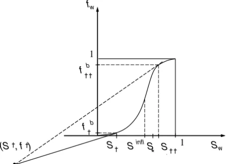
Figure 4 – FindingS∗ from second equality in Eq. (47), by a solid line with slope
ϕHwb/(Hrb+ϕHwb); dashed bounding lines through(0,0)and(S∗†,0). fw
1
1
w S
(S , f ) S Sinfl S
f b
f b
S *
Figure 5 – Graphical solution of Eqs. (53) and (42) for steam-water bifurcation. See Eq. (54). The solid line represents theSCF shock.
Equating vSCF given by Eq. (53) with Eq. (42), making fgb = 1−fwb,
Sg =1−Sw, we obtain
∂fwb ∂Sw(S†)=
fwb(S†)−f†
where
S†= H
b
r/ϕ+HgB HB
g −Hwb
, f†= H
B g HB
g −Hwb
, (55)
and all quantities are evaluated at the boiling temperatureTb. The physics of water at normal pressure dictates that at the boiling temperature,HB
g < Hwb, thus S†<0 and
f†<0. (56)
Remark 11. Since for steam–water (S†, T†) satisfies the inequalities (56),
there is another solution point(S††, f††b)for Eq. (53) closer to (1,1) as shown in Fig. 5. However, it does not play any role in the Riemann solution of the current problem because it exceedsS∗, according to Remark 10.
The contact bifurcationS† separates different wave structures in the steam-water zone as can be seen in Fig. 6.
speed
s
*
v
SCFs
1
w inj
constant constant +
rarefaction
v
b sv
TSCFs
v
gb ,wI II III
Figure 6 – Structure of the steam-water zone below solid curve marked byvsb, vTSCF,
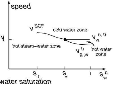
vSCF,vbg,wgiven in Eqs. (25), (42) withSw=S†, Eq. (42) withS†< Swinj < S∗, and Eq. (26) respectively. The figure is not drawn to scale.
In Figures 11 and 2, we show the characteristic speedvSCF andubfor each
Sb
w, at temperatureTbfor fixedu0. As we shall see in Section 4.2, the diagram
Remark 12. By inspection of Figure 5, we see that slightly above S† there existS+and slightly belowS†there existS−, such that in the limit asS+=S−
we havevSCF(S
+)=vSCF(S−)larger thanvSCF(S†), satisfying as well
(S+−S†)vSCF(S+) = u
b
ϕ(f b
w(S+)−f†)
(S−−S†)vSCF(S−) = u
b
ϕ(f b
w(S−)−f†)
Subtracting these two equations, dividing by(S+−S−)and taking the limit as
S+, S−→S†we recover that
ub ϕ
∂fwb
∂Sw(S†)=v
SCF, (59)
and obtain thatS† maximizesvSCF, as illustrated in Figures 3, 6 and 11. An analogous argument holds atS††.
Remark 13. TheSCF shocks are represented in Figure 5 as segments with slope(vSCF/ub)between(S†, f†)and(S, f )for 0
≤S ≤S†. We see that asS
increasesvSCF decreases and the shock amplitudeS−S†increases.
Remark 14. We have shown that(vSCF/ub)has an extremum atS†; the Figure
5 shows that this slope has an extremum atS††. Thus(vSCF/ub) also has an extremum atS††.
3.3 Waves in the liquid water region
Because the initial reservoir temperature isT0, the liquid water region must always contain a cold water zone at temperatureT0far away from the place where
hot steam is injected. If the liquid water region receives water at temperature
Tbfrom the steam zone, the liquid water region consists of a hot liquid water
zone at temperatureTband a cold water zone at temperatureT0, separated by a cooling discontinuity that moves with speedvwb,0given by Eq. (35). This cooling
discontinuity exists providedvb,0
w > vg,wb from Eq. (26) i.e. the hot isothermal
the steam saturation becomes zero and the cooling shock where the temperature jumps to the ambient temperature are separated. See regionS > S∗in Fig. 3.
On the other hand, ifvb,0
w > vg,wb were to be violated, there would be no hot
water zone and no cooling discontinuity. See regionS < S∗in Fig. 3, where there is a steam condensation front instead of a cooling discontinuity.
3.4 Waves in the hot steam zone
The waves in this zone can be found by a pure Buckley-Leverett or Ole˘ınik analysis of Eq. (24), with onecaveat. In the sequence of zones starting at the injection well, the first zone is a steam zone, and the last one is a cold water zone, with heat flow governed by the system (29)–(30). The cold water zone is reached either via a steam condensation shock or via a cooling shock. In the latter case, if there is no other shock between the steam zone and the cold water zone, all waves in the steam zone must have speeds that do not exceed the cooling shock speedvb,0
w given by Eq. (34). In particular, if there is aH I SW shock with speed
given byvbg,w in Eq. (26), we must havevg,wb ≤ vwb,0. Similarly, if there is a saturation rarefaction wave with speed given byvbs in Eq. (25), we must have vb
s ≤vwb,0, the cooling contact discontinuity velocity.
Because of Theorem 1, we see that the restrictions above are satisfied precisely for saturationSb
w in the hot water zone with values between[S∗,1], see Figure 11. For steam–water at the conditions considered in this work, one can verify that the steam water bifurcation water saturationS†is smaller thanS∗in Fig. 5. BecauseS†< S∗, there are no Buckley-Leverett shocks between[Swc, S∗]. This is so because belowS†there are no shocks as rarefaction wave velocities increase monotonically fromSwctoS†. AtS†the velocity is equal to theSCF velocity. BetweenS† and S∗ there are no shocks as the rarefaction wave velocities are larger than theSCF velocity.
Another case of interest occurs if pure steam is injected,i.e. Sw = Swc, the connate water saturation. In this case, a saturation rarefaction wave starts at
x = 0 in the steam zone. A mixture of steam and water can also be injected. As long asSwinj < S†, atx =0 there is a constant state followed by a saturation
compatibility condition:
uinj ϕ
∂fb w(Sw) ∂Sw ≤v
SCF
. (60)
4 Construction of the Riemann solution
Here we describe a systematic way of constructing the Riemann solution through awave curve. Then we summarize the resulting Riemann solution.
S S
* Sw
1
I II III
ub u0
b
Figure 7 – Speedu0for fixedTb,uinj, obtained from Eq. (7) and Fig. 2.
4.1 The wave curve
Let us fix the initial state of the reservoir asS0
w =1,T =T0,u=u0, which is
necessarily the rightmost constant state in the Riemann solution. It turns out to be convenient for the discussion to imagine that an arbitrary value foru0has been specified. Let us decrease the injection saturationSwinj(at the boiling temperature) fromSw =1 toSw =Swc; in our case this corresponds to changingSwb, the water
saturation at theH I SW shock with speed given in Eq. (26). For eachSinj w , we
construct the sequence of elementary waves (and constant states) with decreasing speeds from right to left, that is fromS0
w toSwb. There is a constant state to the
left ofSwb, so there is no other wave to the left ofSwb, the steam shock. For each
Sb
w, we mark its wave speed, forming the solid curves in Fig. 11. This sequence,
Figure 8 – Two cases of steam injection: at connate water saturationSwcor at a low water saturation. With injection atSwcthere is a rarefaction wave and aSCF. With injection
of low water saturation aboveSwcthere is a constant state before the rarefaction.
shocks involved. On rarefaction segments of this backward wave curve, the characteristic speed decreases, while on shock segments of this wave curve, the shock speed increases [8], [14]. We refer to Fig. 11.
WhenSinj
w lies betweenS∗ and 1, the wave with fastest possible speed is the cooling shock in the liquid water region (see Section 3.4), so the backward wave curve corresponds to such a shock wave, with speed given byvwb,0in Eq. (35).
There is a hot steam-water region and a cold water zone. In the hot steam-water region, generically there is a Buckley-Leverett rarefaction-shock and a constant state. The hot steam-water region terminates with theH I SW shock.
The analysis from now on relies on the fact that for steam–water in the actual reservoir,Sinf l < S
∗. ForSwinjwithin(S†, S∗), the wave with slowest speed is the
Figure 9 – Steam injection at intermediate water saturation. We get a constant state upstream and the steam condensation front. TheSCF moves faster than in Figure 8.
vSCF, so there can be no rarefactions nor shocks to the left of theSCF. Thus, forSinj
w in such range, the solution (from left to right) consists of a constant state
of steam and water at temperatureTb, a SCF jumping fromSinj
w to 1.0, and a
constant cold water zone.
Recall that S† < Sinf l. Therefore, from Sinj
w within (Swc, S†), the slowest
speed is a hot steam–water rarefaction speedvsb, which is smaller thanvSCF (vsb
andvSCF coincide at the left stateS†), so there are rarefactions to the left of the SCF. Thus the solution consists of a constant state with saturationSwinj as in the previous case (this constant state disappears ifSwinj =Swc), a rarefaction wave
fromSinj
w toS†, aSCF fromS†to 1, and a constant cold water zone.
Let us explain how the Darcy velocityubis constructed for each value ofSwinj. IfSinj
w lies in the interval (S∗,1),ub is given by Eq. (34), and the speed vb,0w
of the cooling shock is given by Eq. (35) (CaseIII). (As explained in Section 2.1, the velocityuis constant in the hot region and equalsub.) IfSinj
Figure 10 – Steam injection at a high water saturation. We get a constant state upstream, the Buckley-Leverett-saturation shock and the cooling discontinuity. These two waves have distinct speeds; they are both faster than theSCF in Figure 9.
intervalS†andS∗,ub is given by Eq. (44). The speed of theSCF is given by Eq. (45), (CaseII).
IfSinj
w lies in the interval(Swc, S†)(CaseI, sinceubhas to match at the boundary
of CasesI andII,ubis given by Eq. (45) withSw replaced byS†. Thusubis independent ofSinj
w in CaseI.
A summary of the behavior ofub(Swinj)is presented in Fig. 2. Hereub(Swinj)is the value ofubcalculated in the previous paragraphs for a fixedu0.
speed
w
S
S
c
S
S
*
S
1
I II III
S
inflIII
v
s
v
SCFb b
v
b, 0v
b, 0w
w
Figure 11 – Wave speed diagram for left states(Swb, Tb, ub)reachable from the right state(1, T0, u0); for this right state the curve marked vSCF is the Rankine-Hugoniot curve projected onto the(Sw, v)plane. The velocity of the SCF isvSCF (Eq. (42)),vsb
is the hot region saturation characteristic speed (Eq. (25)), andvwb,0is the velocity of the cooling contact discontinuity (Eq. (35)).
u0(Swinj)for specifieduinj, as follows:
ub(Swinj) u0 =
uinj
u0(Sinj w )
. (61)
From this equation we recoveru0(Swinj), essentially by inverting the variable represented in the ordinate in Fig. 2. Thus we obtain Fig. 7.
4.2 Summary of the Riemann solution
The solution consists of three parts, viz. a hot region (A) at constant boiling temperature, an infinitesimally thin cooling front (B) or discontinuity, where all possible steam condensation occurs, and a cold liquid water region downstream (C). See Figure 1.
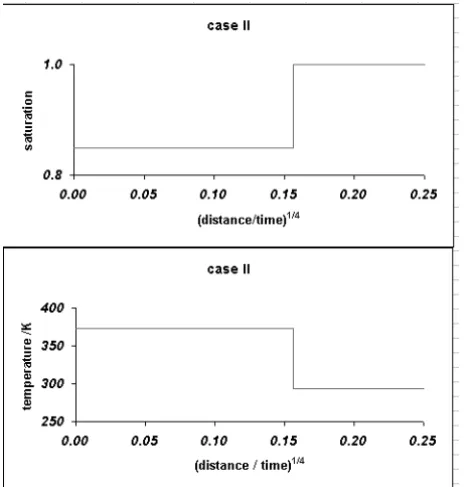
As we have seen, the nature of the solution changes and there are three possible cases (I), (II), and (III), depending on the injected steam qualitySginj =1−Swinj.
Case (I) occurs when the saturation wave velocityvsb(Swinj;uinj)≤vSCF (see Eq. (25)); it consists of a sequence of a constant state at the injection end, ararefaction wave in the hot steam zone (A) ending with saturationS† at the
SCF (B) with speed vSCF defined by saturationsS† andSw = 1, and a cold water constant state in (C). The constant state in (A) disappears if the injection saturation isSwc, that is, pure steam is injected. See Fig. 8. The rarefaction disappears forvb
s(Swinj;uinj)=vSCF, as in this caseSwinj =S†.
Case (II) occurs forvg,wb (Swinj, uinj) < vSCF < vsb(Swinj;uinj); see Eqs. (25), (26) and (27). This case consists of a hot constant steam–water state in (A), the
SCF (B) with speedvSCF defined by left and right saturationsSinj
w and 1 (see
Eq. (45)), and a constant cold water state in (C). See Fig. 9.
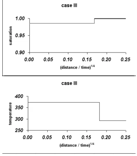
Case (III) occurs for a typically small region for the cooling contact disconti-nuity velocityvwb,0(given in Eq. (35)) withvwb,0> vbg,w(Swinj, uinj)(see Eq. (26)), i.e. the hot isothermal steam-water shock velocity. In this case, there is noSCF. In the hot region (A) there is a constant state with steam-water, then another constant state of pure hot water at the same boiling temperature, separated by a Buckley-Leverett shock. Then there is a cooling shock with speedvb,0
w , where
the saturation of water is constant (Sw =1) and the temperature changes from
Tbto the reservoir temperatureT0. (See Fig. 10.)
Figure 6 illustrates the saturation dependence of the various velocities that are the basis of the steam-water zone structure, for Cases (I), (II), (III).
5 Lax conditions for the steam condensation front
Despite the fact that our system does not satisfy Lax’s theorem hypotheses, we will compare theSCF speed to the left and right characteristic speeds. We will conclude that from the point of view of Lax’s inequalities, theSCF is a 2-shock or a limit of such shocks.
We introduce the heat capacitiesCp(T )as the temperature derivatives of the enthalpies [J/m3] at constant pressure,i.e. Cp
w(T )is the heat capacity of water
andCgp(T )is the heat capacity of steam. In the same way we define the thermal
Eqs. (21)–(22) may be written in quasilinear form as:
−∂u
∂x(ρwfw+ρgfg)= −ϕ
(Swρwαw+Sgρgαg)∂T ∂t
+ρg−ρw∂Sw
∂t
−u
fwρwαw+fgρgαg
+ρg−ρw∂fw/∂T∂T ∂x −
(ρw−ρg)∂fw ∂Sw ∂Sw ∂x , (62)
q0−∂u
∂x(Hwfw+H s
gfg)=ϕ
Crp
ϕ +SwC p w+SgC
p g
∂T ∂t
+Hw−Hgs∂Sw
∂t
+u
fwCwp+fgCgp
+(Hw−Hgs)∂fw/∂T
∂T
∂x +
(Hw−Hgs) ∂fw ∂Sw ∂Sw ∂x . (63)
We restrict our attention to regions where∂u/∂x=0 andq =0, that is, away from any kind of shocks. Thus, the LHS terms of Eqs. (62), (63) vanish.
We let
AI = C
p r
ϕ +SwC p w+SgC
p g,
AI I = fwCwp+fgCgp+(Hw−Hgs)∂fw/∂T .
(64)
Multiplying the RHS of Eq. (62) by−(Hw−Hs
g)and of Eq. (63) by(ρw−ρg)
and adding leads to a new equation, which will be used instead of Eq. (63):
ϕ
(Hw−Hgs)(Swρwαw+Sgρgαg)+ρw−ρgAI
∂T ∂t
+u
(Hw−Hgs)
fwρwαw+fgρgαg+(ρg−ρw)∂fw/∂T
+(ρw−ρg)AI I
∂T ∂x =0.
(65)
We let
AI V =
Hw−Hgs
(fwρwαw+fgρgαg+(ρg−ρw)∂fw/∂T )
+ρw−ρgAI I
.
(67)
Thus in regions where∂u/∂x=0 andq =0, that is, away from any kind of shocks (see Remarks 1 and 2), Eqs. (62)–(65) may be written in matrix form as:
A∂ ∂t +B
∂ ∂x
S
T =0. (68)
Letµbe a characteristic speed. Then the determinant of the following matrix must vanish:
−µϕ
ρg−ρw
(Swρwαw+Sgρgαg)
0 AI I I
+u
ρg−ρw∂fw/∂Sw fwρwαw+fgρgαg+(ρg−ρw)(∂fw/∂T )
0 AI V
.
(69)
Since the matrix above is upper triangular, the characteristic speeds are easily read from the diagonals:
µ= u
ϕ ∂fw
∂Sw and µ=
u ϕ
AI V
AI I I. (70)
(It is easy to check thatAI I I never vanishes.)
Now, in the liquid water region on the right of the SCF,Sg = 0, fg = 0,
∂fw
∂Sw =0, the characteristic speeds are
µ=0 and v0= C
p w(T0) Crp(T0)+ϕCw(Tp 0)
u0. (71)
The latter speed has already been calculated in Eq. (46).
On the other hand, in the hot steam zone the characteristic speeds are
vbs = u
b
ϕ ∂fb
w
∂Sw, and v
b T =
ub ϕ
AI V(Tb)
AI I I(Tb). (72)
For a(−)state for theSCF withSwin(S∗, S†)we have that the thermal char-acteristic speed in the steam zone satisfies 0< v0 < vSCF, and the steamfront velocity satisfiesvTb < vSCF < vb
s, so the SCF would be called a 2-shock in
Lax’s classification scheme. However, Lax’s theorem only applies to shocks with small amplitude, while theSCF is a large shock, and only if the governing equations were a system of conservation laws satisfying appropriate technical hypotheses, such as genuine nonlinearity, which is actually violated at the in-flectionSinf l. Moreover, even the Lax inequalities are violated starting at the steam-water bifurcation; there is no conclusive mathematical evidence that the
SCF shock needed to complete the Riemann solution is physically admissible. This is the issue left open.
6 Summary and conclusions
A complete and systematic description of all possible solutions of the Riemann problem for the injection of a mixture of steam and water into a water-saturated porous medium, for all possible reservoir temperatures and pressures below the water critical point. For each Riemann data, we found a unique solution.
As determined by the dissipative effects of capillary porous forces combined with the mass source term given in Eq. 3, the internal structure of theSCF is consistent with the Riemann solution in this work. This fact is demonstrated in a companion paper [4].
7 Acknowledgments
This work was partially done at IMA, University of Minnesota, and therefore partially funded by NSF. H.B. thanks Shell for the continuous support of the steam drive recovery research at the Delft University of Technology. We also thank Beata Gundelach for careful and expert typesetting of this paper. We thank the referees for suggestions that improved the paper.
Appendix A – Physical quantities; symbols and values
Physical quantity Symbol Value Unit
Water, steam fractional
functions fw, fg Eq. (9). [m3/m3] Water-steam frac. flow,
hot region fwb,fgb [m3/(m2s)] Porous rock permeability k 1.0×10⁻¹² [m2] Water, steam relative
permeabilities krw, krg Eq. (82), (82). [-]
Pressure p 1.0135×10⁵ [Pa]
Mass condensation rate q Eq. (3). [kg /(m3s)] Mass condensation
rate coefficient qb 0.01 [kg /(m3sK)] Steam injection rate uinj 9.52 ×10⁻⁴ [m3/(m2s)] Water, steam phase velocity uw, ug Eq. (2). [m3/(m2s)] Total Darcy velocity u uw+ug, Eq. (13). [m3/(m2s)] Flow rate in hot region ub Eq. (24), (34). [m3/(m2s)] Flow rate in cold water zone u0 Eq. (31). [m3/(m2s)]
SCFvelocity vSCF Eq. (42). [m/s]
Cooling contact disc. speed,
hot water zone vbw Eq. (36). [m/s]
Thermal characteristic speed,
cold water zone v0 Eq. (46). [m/s]
Saturation characteristic speed,
hot region vbs Eq. (25). [m/s]
Hot isothermal steam-water
shock velocity vbg,w Eq. (26). [m/s] Cooling contact
discontinuity velocity vb,0w Eq. (35). [m/s] Water, steam heat capacity∗ Cwp, Cgp dHw/dT , dHgs/dT [J/(m3K)] Effective rock heat capacity Crp 2.029×10⁶ [J/(m3K)] Steam enthalpy Hg ρg(T )hg(T )−hw(T0) [J/m3] Steam sensible heat Hgs Eq. (77). [J/m3] Steam latent heat Hgl ρg(T )0 [J/m3] Rock enthalpy Hr ρrCrp(T −T0) [J/m3] Water enthalpy Hw ρw(T )hw(T )−hw(T0) [J/m3] Water, rock enthalpy
at boiling temperature Hwb,Hrb Hw(Tb),Hr(Tb) [J/m3] Steam total, sensible enthalpy
at boil. temp. HgB,Hgb Eq. 43. [J/m3]
Physical quantity Symbol Value Unit
Water, rock enthalpy,
reservoir temperature Hw0,Hr0 Hw(T0),Hr(T0) [J/m3] Water, steam saturations Sw, Sg Dependent variables. [m3/m3] Connate water saturation Swc 0.15 [m3/m3] Water injection saturation Swinj See Section 4. [m3/m3] Hot-cold bifurcation
water saturation S∗ Theorem 1. [m3/m3] Steam-water bifurcation
water saturation S† Eq. (53). [m3/m3] Steam-water bifurcation
ghost saturation S†† See Remark 11. [m3/m3] Water saturation at inflection Sinf l Frac. flow infl. sat. [m3/m3]
Temperature T Dependent variable. [K]
Reservoir temperature T0 293. [K]
Boiling point of water–steam Tb Eq. (73). [K] Steam thermal expansion coefficient∗ αg −(1/ρg)(∂ρg/∂T )p [/K] Water thermal expansion coefficient αw −(1/ρw)(∂ρw/∂T )p [/K] Water, steam thermal conductivity κw,κg 0.652, 0.0208 [W/(mK)] Rock, composite thermal conductivity κr,κ 1.83, Eq. (7). [W/(mK)] Saturation exponent forPc λs 0.5, Eq. (83) [-] Water, steam viscosity µw,µg Eq. (79), Eq. (78). [Pa s] Water, steam densities ρw,ρg Eq. (81), Eq. (80). [kg/m3] Water, steam, rock densities
– boiling temp. ρbw,ρgb,ρbr Eq. (32) [kg/m3] Water, steam, rock densities
– reservoir temp. ρ0w,ρg0,ρr0 [kg/m3] Interfacial tension σwg 58 ×10−3 [N/m]
Rock porosity ϕ 0.38 [m3/m3]
Water evaporation heat
at reservoir temperature 0 Eq. 1. [J/kg] Capillary diffusion coefficient Eqs. (11), (12). [m3/m3]
functions. For convenience we express the heat capacity of the rockCrpin terms
of energy per unit volume ofporous mediumper unit temperaturei.e.the factor 1−ϕ is already included in the rock density. All other densities are expressed in terms of mass per unit volume of the phase.
A.1 Temperature dependent properties of steam and water
We use reference [16] to obtain all the temperature dependent properties below. The water and steam densities used to obtain the enthalpies are defined at the bottom. First we obtain the boiling pointTbat the given pressurep,i.e.
Tb=280.034+ℓ(14.0856+ℓ(1.38075+ℓ(−0.101806+0.019017ℓ))), (73)
whereℓ =log(p)andpis the pressure in [k Pa]. The evaporation heat [J/kg] is given as a function of the temperatureT at which the evaporation occurs. We use atmospheric pressure (p= 101.325 [k Pa]) in our computations, to make the example representative of subsurface contaminant cleaning.
The liquid water enthalpyhw(T )[J/kg] as a function of temperature is approx-imated by
hw(T ) = 2.36652×10⁷−3.66232×10⁵T +2.26952×10³T2
−7.30365T3+1.30241×10⁻²T4−1.22103×10⁻⁵T5
+4.70878×10⁻⁹T6.
(74)
The steam enthalpyhg[J/kg] as a function of temperature is approximated by
hg = −2.20269×10⁷+3.65317×10⁵T −2.25837×10³T2
+7.3742T3−1.33437×10⁻²T4+1.26913×10⁻⁵T5
−4.9688×10⁻⁹T6.
(75)
For the latent heathlg[J/kg] or evaporation heat(T )we obtain
hlg =
7.1845×10¹²+1.10486×10¹⁰T −8.8405×10⁷T2
+1.6256×10⁵T3−121.377T4 1 2.
(76)
The sensible heat of steamHs
g(T )in [J/m
3] is given as Hgs(T )=ρg
hg(T )−hw
T0
−
T0
We also use the temperature dependent steam viscosity
µg = −5.46807×10⁻⁴+6.89490×10⁻⁶T −3.39999×10⁻⁸T2
+8.29842×10⁻¹¹T3−9.97060×10⁻¹⁴T4
+4.71914×10⁻¹⁷T5.
(78)
The temperature dependent water viscosityµwis approximated by
µw = −0.0123274+27.1038
T −
23527.5
T2 +
1.01425×10⁷ T3
−2.17342×10
9
T4 +
1.86935×10¹¹
T5 .
(79)
For the steam density as a function of temperatureT[K]we use a different expression than [16] because our interest is a steam density at constant pressure, which is not necessarily in equilibrium with liquid water.
ρg(T )=pMH2O
ZRT (80)
wherep is the total pressure at which the steam displacement is carried out,
R=8.31 [J/mol K] and Z is the Z-factor (see e.g. Dake [6]) and MH2O =
0.018kg/mole is the molar weight of water. For the atmospheric pressures of interest here the Z-factor is close to unity. The liquid water density as a function of the temperatureT[K]is given as
ρw(T ) = 3786.31−37.2487T +0.196246T2−5.04708×10⁻⁴T3
+6.29368×10⁻⁷T4−3.08480×10⁻¹⁰T5. (81)
A.2 Constitutive relations
We use a porosityϕthat is representative for unconsolidated sand. The relative permeability functionskrwandkrgare considered to be power functions of their respective effective saturations [7],i.e.
Swe=(Sw−Swc)/(1−Swc), Sge =Sg/(1−Swc).
water permeability and a quadratic dependence for the steam relative permeabil-ity.
The relative permeability functionskrw and krg are considered to be power functions of their respective saturations [7],i.e.
krw =
Sw−Swc
1−Swc
nw
for Sw ≥Swc,
0 for 0≤Sw ≤Swc,
krg =
Sg
1−Swc
ng
.
(82)
For the computations we takenw =4,ng =2.The connate water saturation
Swcis given in the table.
The capillary pressure is of the Brooks-Corey type based on the dimensionless capillary pressure fromPc(Sw =0.5)/
σwg√ϕ/ k
=0.5. The capillary pres-sure between steam and water is given by the empirical expression which com-bines Leverett’s approach to non-dimensionalize the capillary pressure [9] with the semi-empirically determined saturation dependence suggested by Brooks [3]:
Pc =σwgγ
ϕ k
1
2−Swc
1−Swc 1
λs
Sw −Swc
1−Swc
−λs1
, (83)
whereγ is a parameter that in many cases assumes values between 0.3 and 0.7. We use γ = 0.5 andλs = 12. Finally σwg = 0.058 N/m is the water-vapor interfacial tension. We disregard its temperature dependence and use the value at the boiling point (see [17], p. F-45).
REFERENCES
[1] A. Ali Cherif, A. Daïf,Etude numérique du transfert de chaleur et de masse entre deux plaques planes verticales en présence d’un film de liquide binaire ruisselant sur l’une des plaques chauffée, Int. J. Heat and Mass Transfer42(1999), 2399–2418.
[2] J. Bear,Dynamics of Fluids in Porous Media, p. 650 and 651, Dover Publications, Inc., New York (1972).
[3] R.B. Bird, W.E. Stewart and E.N. Lightfoot,Transport Phenomena, John Wiley & Sons (1960). [4] R.H. Brooks and A.T. Corey,Properties of porous media affecting fluid flow, J. Irr. Drain.
[5] J. Bruining, D. Marchesin and S. Schecter,Steam condensation waves in water-saturated porous rocks, in preparation, 2002.
[6] J. Bruining, D. Marchesin and C.J. Duijn,Steam injection into water-saturated porous rock, IMPA preprint 136/2002, 2002.
[7] L.P. Dake,Fundamentals of Reservoir Engineering, Elsevier Science Publishers, Amsterdam, 1978.
[8] F.A.L. Dullien,Porous media; fluid transport and pore structure, Academic Press, N.Y. (1979). [9] E. Isaacson, D. Marchesin, B. Plohr and J.B. Temple,Multiphase flow models with singular
Riemann problems, Mat. Apl. Comput.,112 (1992), 147-166.
[10] M. C. Leverett,Capillary behavior in porous solids, Trans., AIME,142(1941), 142-169. [11] O. Ole˘ınik,Discontinuous Solutions of Nonlinear Differential Equations, Usp. Mat. Nauk.
(N.S.) v.12, pp. 3-73, 1957. English transl. in Amer. Math Soc. Transl. Ser.226, 95-172. [12] P.F. Peterson, Diffusion Layer Modeling for Condensation with Multicomponent
Non-condensable Gases, Journal of Heat Transfer, Transactions of the ASME, Vol122(2000), 716-720.
[13] G.A. Pope,The application of fractional flow theory to enhanced oil recovery, SPEJ, 191-205, June 1980.
[14] M. Prats,Thermal Recovery, Monograph Series, SPE, Richardson, TX,7(1982).
[15] S. Schecter, D. Marchesin and B. Plohr,Classification of codimension-one Riemann solutions, Journal of Dynamics and Differential Equations, vol.133 (2001), pp. 523-588.
[16] A. Shoda, C.Y. Wang and P. Cheng,Simulation of constant pressure steam injection in a porous medium, Int. Comm. Heat Mass Transfer Vol256 (1998), 753-762. (1998). [17] W.S. Tortike and S.M. Farouq Ali,Saturated-steam-property functional correlations for fully
implicit reservoir simulation, SPERE (November 1989) 471-474.