UNIVERSIDADE DE LISBOA FACULDADE DE CIÊNCIAS
The Family Traveling Salesman Problem
“ Documento Definitivo”
Doutoramento em Estatística e Investigação Operacional
Especialidade de Otimização
Raquel Monteiro de Nobre Costa Bernardino
Tese orientada por:
Professora Doutora Ana Maria Duarte Silve Alves Paias
UNIVERSIDADE DE LISBOA FACULDADE DE CIÊNCIAS
The Family Traveling Salesman Problem
Doutoramento em Estatística e Investigação Operacional
Especialidade de Otimização
Raquel Monteiro de Nobre Costa Bernardino
Tese orientada por:
Professora Doutora Ana Maria Duarte Silve Alves Paias
Júri: Presidente:
● Doutora Maria Eugénia Vasconcelos Captivo, Professora Catedrática, Faculdade de Ciências da Universidade de Lisboa; Vogais:
● Doutora Maria Cristina Saraiva Requejo Agra, Professora Auxiliar, Departamento de Matemática da Universidade de Aveiro;
● Doutor José Manuel Vasconcelos Valério de Carvalho, Professor Catedrático, Escola de Engenharia da Universidade do Minho;
● Doutor José Manuel Pinto Paixão, Professor Catedrático, Faculdade de Ciências da Universidade de Lisboa; ● Doutor Luís Eduardo Neves Gouveia, Professor Catedrático, Faculdade de Ciências da Universidade de Lisboa; ● Doutora Maria Eugénia Vasconcelos Captivo, Professora Catedrática, Faculdade de Ciências da Universidade de Lisboa; ● Doutora Ana Maria Duarte Silva Alves Paias, Professora Auxiliar, Faculdade de Ciências da Universidade de Lisboa (orientadora).
Documento especialmente elaborado para a obtenção do grau de doutor
O meu sincero obrigada à Professora Doutora Ana Maria Duarte Silva Alves Paias, a minha orien-tadora. A sua dedicação a esta dissertação fez com que esta chegasse a bom porto. Obrigada pela paciência, disponibilidade e por estar sempre disposta a ensinar-me. Foi mais uma vez uma honra tê-la como minha orientadora.
Um grande obrigada à minha família. Aos meus pais, que sempre me tentaram educar da melhor forma possível e fizeram de mim aquilo que sou hoje. Um obrigada especial ao meu pai, que nestes últimos anos sempre me incentivou a aprender mais e me proporcionou esta aventura que foi o doutoramento. Aos meus avós, Babá e Avô Júlio, obrigada por ainda hoje tomarem conta de mim. Daniel, obrigada! Obrigada pelo teu companheirismo durante esta etapa e por, mais uma vez, acreditares que isto seria possível antes de mim. Conseguimos, que venha o próximo desafio.
Gostaria também de agradecer a todos os professores que me acompanharam neste percurso. Um agradecimento especial ao professor Luís Gouveia, pois também contribuiu de forma indireta para esta dissertação.
Um obrigada especial aos meus colegas de gabinete e de almoço, Michele e Jessica pelas dis-cussões interessantes que tivemos e pelos bons tempos que passámos juntos.
Por fim, a todos os que de uma forma ou de outra me incentivaram durante o decorrer desta dissertação nem que seja por perguntarem como está a correr, o meu mais sincero obrigada.
Consider a depot, a partition of the set of nodes into subsets, called families, and a cost matrix. The objective of the family traveling salesman problem (FTSP) is to find the minimum cost circuit that starts and ends at the depot and visits a given number of nodes per family. The FTSP was motivated by the order picking problem in warehouses where products of the same type are stored in different places and it is a recent problem. Nevertheless, the FTSP is an extension of well-known problems, such as the traveling salesman problem.
Since the benchmark instances available are in small number we developed a generator, which given a cost matrix creates an FTSP instance with the same cost matrix. We generated several test instances that are available in a site dedicated to the FTSP.
We propose several mixed integer linear programming models for the FTSP. Additionally, we establish a theoretical and a practical comparison between them. Some of the proposed models have exponentially many constraints, therefore we developed a branch-and-cut (B&C) algorithm to solve them. With the B&C algorithm we were able to obtain the optimal value of open benchmark instances and of the majority of the generated instances.
As the FTSP is an NP-hard problem we develop three distinct heuristic methods: a genetic algorithm, an iterated local search algorithm and a hybrid algorithm. With all of them we were able to improve the best upper bounds available in the literature for the benchmark instances that still have an unknown optimal value.
We created a new variant of the FTSP, called the restricted family traveling salesman problem (RFTSP), in which nodes from the same family must be visited consecutively. We apply to the RFTSP the methods proposed for the FTSP and develop a new formulation based on the interfamily and the intrafamily relationships.
space
Keywords: Family traveling salesman problem; Multicommodity flow; Projections;
Considere-se um depósito, uma partição do conjunto de cidades em vários subconjuntos, aos quais chamamos famílias, e custos de deslocação entre o depósito e as cidades e entre as várias cidades. O objetivo do family traveling salesman problem (FTSP) é determinar o circuito elementar de custo mínimo que começa e acaba no depósito e visita um número predeterminado de cidades em cada família. O FTSP foi motivado pelo problema de recolha de produtos em armazéns onde os produ-tos do mesmo tipo estão armazenados em locais diferentes. O FTSP é um problema relativamente recente pois, além do artigo desenvolvido no âmbito desta dissertação, existe apenas um artigo na literatura sobre o mesmo. Contudo, o FTSP pode ser visto como uma generalização de problemas bem conhecidos da literatura, como o problema do caixeiro viajante e o problema do caixeiro vi-ajante generalizado (generalized traveling salesman problem), daí a importância do seu estudo no âmbito de uma dissertação de doutoramento.
Como as instâncias do FTSP disponíveis na literatura são em número reduzido decidimos criar um gerador de instâncias para o FTSP. Este gerador recebe uma matriz de custos e cria quatro instâncias diferentes do FTSP, que diferem no número de visitas por família, com a mesma matriz de custos. As quatro instâncias foram geradas para terem características diferentes, nomeadamente criámos um tipo de instância para ter um número reduzido de visitas por família e outro tipo para ter um número elevado de visitas por família. Para gerarmos novas instâncias do FTSP usámos matrizes de custos, simétricas e assimétricas, de instâncias de referência do problema do caixeiro viajante e de instâncias de referência assimétricas do problema do traveling purchaser. Criou-se um site dedicado ao FTSP no qual se disponibilizam para toda a comunidade científica todas as instâncias existentes do FTSP, nomeadamente as instâncias de referência da literatura e as instâncias geradas. Nesta dissertação apresentamos vários modelos de programação linear inteira mista para o FTSP. Estes modelos são comparados empiricamente e através de resultados teóricos. Alguns dos mode-los propostos contêm conjuntos de restrições que são em número exponencial, pelo que temos de recorrer a um algoritmo de branch-and-cut, que combina um algoritmo de branch-and-bound com um algoritmo de planos de corte, para os resolver. Pela experiência computacional verificámos que os modelos com um número exponencial de restrições são os mais eficientes. O melhor
mod-nação de subcircuitos propostas por Dantzig et al. (1954) para o problema do caixeiro viajante e as desigualdades RFV, criadas no âmbito desta dissertação para o FTSP. Estas últimas garantem que se num subconjunto de cidades que contém o depósito, designado por S′, não existem cidades sufi-cientes para satisfazer as visitas de uma determinada família, então teremos que visitar uma cidade no conjunto complementar de S′. Ambas as desigualdades eliminam subcircuitos contudo, como a separação das desigualdades RFV é muito demorada, usamos as desigualdades CC para eliminar subcircuitos e as desigualdades RFV são adicionadas como desigualdades válidas para melhorar o valor da relaxação linear. Foi ainda incorporado no algoritmo de branch-and-cut um método heurís-tico muito simples que permite obter uma solução admissível para o FTSP (não necessariamente a ótima). Deste modo garantimos que, com o algoritmo de branch-and-cut, conseguimos sempre obter uma solução admissível para o problema. Com o algoritmo de branch-and-cut aplicado ao modelo CC+RFV conseguimos obter o valor ótimo de instâncias de referência que tinham valor ótimo desconhecido. No que diz respeito às instâncias geradas, conseguimos obter o valor ótimo de 148 instâncias das 164 instâncias geradas, sendo que a proporção de instâncias simétricas resolvidas é 73% e a proporção de instâncias assimétricas resolvidas é de 99%.
Como o problema do caixeiro viajante pode ser visto como um caso particular do FTSP, em que temos que visitar todas as cidades de todas as famílias, podemos concluir que o FTSP pertence à classe de problemas NP-difícil, pelo que desenvolvemos métodos heurísticos para o FTSP. Nesta dissertação são propostos três métodos heurísticos, nomeadamente: um algoritmo genético, que usa permutações como cromossomas; um algoritmo de iterated local search (ILS), que itera entre um algoritmo de pesquisa local e um algoritmo de perturbação; e um algoritmo híbrido, que combina o modelo CC+RFV proposto com o algoritmo de ILS. Os resultados computacionais mostraram que o algoritmo genético é o algoritmo mais eficiente e que o algoritmo ILS e o algoritmo híbrido são os mais eficazes, pois nas instâncias testadas obtêm sempre uma solução de custo inferior ao da solução obtida com o algoritmo genético. Como o objetivo principal é obter as soluções com o menor custo possível decidimos usar o algoritmo ILS e o algoritmo híbrido, pois nenhum obteve o melhor resultado em todas as instâncias. Comparámos estes dois algoritmos e concluímos que, geralmente, o algoritmo ILS é mais eficiente enquanto que o algoritmo híbrido é mais eficaz. Os métodos heurísticos apenas foram aplicados a instâncias que o método exato não resolveu, isto é, instâncias que têm valor ótimo desconhecido. No que diz respeito às instâncias de referência com valor ótimo desconhecido, conseguimos obter soluções de custo inferior aos melhores limites su-periores disponíveis na literatura para todas as instâncias testadas e usando ambos os algoritmos.
ritmo de branch-and-cut. Das 16 instâncias geradas que têm valor ótimo desconhecido os métodos heurísticos só conseguiram obter uma solução de custo inferior à solução obtida pelo algoritmo de
branch-and-cut em três instâncias. Contudo, a comparação entre o algoritmo de branch-and-cut
e os métodos heurísticos não é justa pois o algoritmo de branch-and-cut obteve as suas soluções ao fim de três horas, enquanto que, por exemplo o algoritmo de ILS, obteve as suas soluções num tempo médio de 20 segundos.
Nesta dissertação também apresentamos uma variante do FTSP que, tanto quanto sabemos, nunca foi apresentada na literatura. A variante do FTSP chama-se restricted family traveling
sales-man problem (RFTSP) e é obtida exigindo que as cidades da mesma família sejam visitadas
con-secutivamente. Para resolver o RFTSP decidimos adaptar os métodos que obtiveram os melhores resultados no FTSP, nomeadamente o algoritmo de branch-and-cut aplicado ao modelo CC+RFV e, relativamente a métodos heurísticos, o algoritmo de ILS e o algoritmo híbrido. Com estes métodos obtivemos os valores ótimos e limites superiores, para as instâncias com valor ótimo desconhecido. Comparando os resultados obtidos para o FTSP e os obtidos para o RFTSP verificamos que, nas in-stâncias assimétricas, o número de inin-stâncias com valor ótimo conhecido baixou significativamente. Das 100 instâncias geradas com custos assimétricos e considerando o RFTSP, apenas conseguimos obter o valor ótimo de 76 instâncias. Ainda relativamente ao RFTSP, propomos um novo modelo de programação linear inteira mista. Este novo modelo explora as relações dentro de cada família e as relações entre famílias como um problema de caminho mais curto e um problema do caixeiro vi-ajante, respetivamente. Este novo modelo tem um número muito elevado de variáveis e restrições o que torna a sua resolução menos eficiente. Contudo, este novo modelo obtém valores de re-laxação linear superiores aos do modelo CC+RFV adaptado, pelo pode ser usado como objeto de investigação futura como ponto de partida para novas abordagens de resolução como por exemplo a utilização de técnicas de decomposição.
space
Palavras-chave: Family traveling salesman problem; Fluxos multicomodidade; Projecções;
1 Introduction 1
2 Mathematical Background 5
2.1 Graph theory . . . 5
2.2 Polyhedral theory . . . 8
2.3 Linear programming theory . . . 12
2.4 Complexity theory . . . 21
2.5 Basic linear programming problems . . . 22
2.5.1 The assignment problem . . . 23
2.5.2 The maximum flow problem . . . 23
2.5.3 The minimum capacity cut problem . . . 24
2.5.4 The shortest path problem . . . 25
3 The Family Traveling Salesman Problem 27 3.1 Literature review . . . 28
3.2 Related problems . . . 29
3.3 Basic constructive heuristics and neighborhoods . . . 30
3.3.1 Constructive heuristics . . . 30
3.3.2 Neighborhoods . . . 31
3.4 Instances . . . 33
4 Mathematical Formulations 37 4.1 A generic formulation for the FTSP . . . 37
4.2 Formulating the subtour elimination constraints . . . 39
4.2.1 Compact formulations . . . 39
4.2.1.1 The single-commodity flow model . . . 40
4.2.2.1 Connectivity cuts model . . . 45
4.2.2.2 Rounded visits model . . . 45
4.2.2.3 Rounded family visits model . . . 49
4.3 Theoretical comparison of the several formulations . . . 53
4.3.1 Comparing the compact models . . . 54
4.3.2 Comparing the compact and the non-compact models . . . 60
4.3.3 Comparing the non-compact models . . . 67
4.4 Empirical comparison of the several formulations . . . 68
4.4.1 Combining the CC inequalities and the RFV inequalities . . . 72
5 The Branch-and-Cut Algorithm 75 5.1 The branch-and-cut algorithm outline . . . 75
5.2 The separation algorithms . . . 76
5.2.1 Separating the CC inequalities . . . 76
5.2.2 Separating the RFV inequalities . . . 81
5.2.3 Separating both the CC and the RFV inequalities . . . 85
5.2.3.1 Separating only some RFV inequalities . . . 87
5.3 Heuristic callback . . . 92
5.4 Computational experiment . . . 94
5.4.1 Benchmark instances . . . 94
5.4.2 Generated instances based on symmetric TSP instances . . . 99
5.4.3 Generated instances based on asymmetric TSP instances . . . 105
5.4.4 Generated instances based on asymmetric UTPP instances . . . 110
6 Heuristic Algorithms 115 6.1 The genetic algorithm . . . 116
6.2 The iterated local search algorithm . . . 124
6.3 The hybrid algorithm . . . 130
6.3.1 Constructive phase . . . 131
6.3.2 Improvement phase . . . 137
6.3.2.1 Transferring information from the constructive phase to the im-provement phase . . . 138
7.2 Basic heuristics and neighborhoods for the RFTSP . . . 151
7.3 Mathematical formulations for the RFTSP . . . 153
7.3.1 Formulating the consecutiveness condition . . . 154
7.3.2 The inter- and intrafamily formulations . . . 154
7.3.2.1 Formulating the intrafamily subproblem . . . 155
7.3.2.1.1 The path single-commodity flow . . . 158
7.3.2.1.2 The path multi-commodity flow . . . 158
7.3.2.1.3 The path connectivity cuts . . . 159
7.3.2.1.4 The path rounded visits . . . 159
7.3.2.2 Formulating the interfamily subproblem . . . 160
7.3.2.3 Theoretical comparison of the inter- and intrafamily formulations 161 7.3.3 Empirical comparison between the adapted formulations and the inter- and intrafamily formulations . . . 162
7.4 The branch-and-cut algorithm for the RFTSP . . . 167
7.4.1 Heuristic callback . . . 168
7.4.2 Computational experiment . . . 169
7.4.2.1 Benchmark instances . . . 169
7.4.2.2 Generated instances based on symmetric TSP instances . . . 171
7.4.2.3 Generated instances based on asymmetric TSP instances . . . 175
7.4.2.4 Generated instances based on asymmetric UTPP instances . . . . 179
7.5 Heuristic algorithms for the RFTSP . . . 183
7.5.1 The iterated local search algorithm . . . 184
7.5.2 The hybrid algorithm . . . 185
7.5.3 Computational experiment . . . 186
8 Conclusion 197 8.1 Main conclusions . . . 197
8.2 Future work . . . 200
A Instance Description 207 B Branch-and-cut algorithm detailed results 217 B.1 Linear programming relaxation results without heuristic separation . . . 217
B.5 Linear programming relaxation results for instance set 3 . . . 224
B.6 Linear programming relaxation results for instances rbg with SCF model . . . 227
B.7 Linear programming relaxation results for instance set 4 . . . 228
C Heuristic algorithms detailed results 231 C.1 Genetic algorithm . . . 231
C.1.1 Results obtained with the GA algorithm . . . 231
C.1.2 Results obtained with the GA+NN algorithm . . . 232
C.1.3 Results obtained with the LS algorithm . . . 233
C.1.4 Results obtained with the LS_random algorithm . . . 233
C.1.5 Results obtained with the LS_insertRemove algorithm . . . 234
C.1.6 Results obtained by applying the LS_insertRemove algorithm to several solutions . . . 235
C.2 Iterated local search algorithm . . . 236
C.2.1 Results obtained with the several choosing criteria of the perturbation method236 C.2.2 Results obtained with the removal criterion Random_removal in the per-turbation method . . . 237
C.2.3 Results obtained combining both removal criteria in the perturbation method 238 C.2.4 Results obtained with different numbers of iterations in the ILS algorithm . 240 C.3 Hybrid algorithm . . . 241
C.3.1 Evaluating the number of visits by using instance bier . . . 241
C.3.2 Results obtained with the several r∗values . . . 242
C.3.3 Results obtained with the several ∆ values . . . 243
C.3.4 Results obtained with the several Λ values . . . 243
C.3.5 Results obtained with the hybrid algorithm . . . 244
C.3.6 Results obtained with the hybrid algorithm with dual information . . . 245
C.4 Final results with different seeds . . . 245
D RFTSP detailed results 251 D.1 Linear programming relaxation results obtained with the adapted formulations for the RFTSP . . . 251 D.2 Linear programming relaxation results obtained with the y-separation for the RFTSP 253 D.3 Linear programming relaxation results obtained with y-separation for the RFTSP . 254
E The Branch-and-Cut Algorithm for the Inter- and Intrafamily Formulations 265
E.1 The separation algorithms . . . 265 E.1.1 Separating the subtour elimination constraints in the interfamily subproblem 266 E.1.2 Separating the P-CC inequalities . . . 268 E.1.3 Separating the P-RV inequalities . . . 272
2.1 Examples of a directed and a nondirected graph. . . 6
2.2 Example of a directed and simple graph. . . 6
2.3 Graphical representation of the Pepolytope. . . 10
2.4 Graphical representation of the Pepolytope without the redundant inequalities. . . 12
2.5 Graphical representation of the set of feasible solutions for the Peproblem. . . 14
2.6 Graphical representation of the convex hull of the set of feasible solutions of the Pe problem. . . 15
2.7 Graphical representation of the formulation Pdual. . . 19
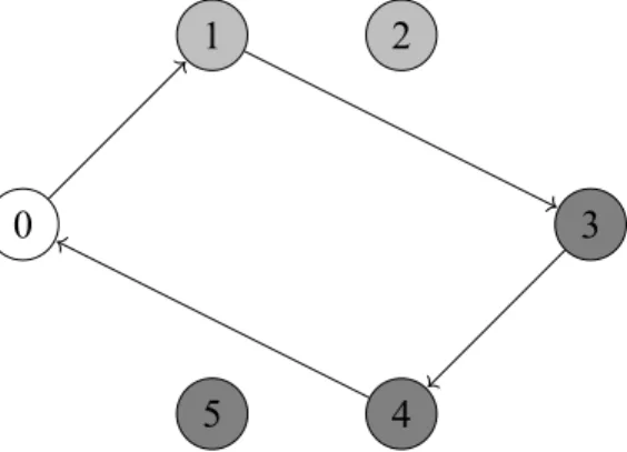
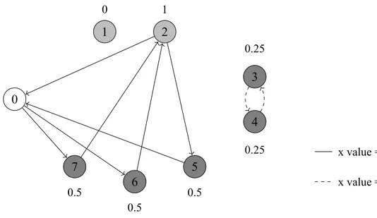
3.1 An example of a feasible solution for an FTSP instance. . . 28
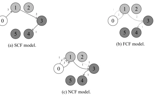
4.1 Representation of the several flow systems. . . 40
4.2 RV inequalities motivation. . . 48
4.3 RFV inequalities motivation. . . 52
4.4 Feasible solution for the LP relaxation of the FCF model. . . 57
4.5 Feasible solution for the LP relaxation of the NCF model. . . 59
4.6 Feasible solution for the LP relaxation of the RV model. . . 61
4.7 Feasible solution for the LP relaxation of the NCF+model. . . 63
4.8 Feasible solution for the LP relaxation of the RFV model. . . 65
4.9 Known relationships between the proposed formulations. . . 68
4.1 Node-commodity flow models summary. . . 44 4.2 Linear programming relaxation results obtained with the compact models. . . 69 4.3 Linear programming relaxation results obtained with the non-compact models. . . 70 4.4 Linear programming relaxation results obtained with the CC+RFV model. . . 72
5.1 Heuristic separation CC inequalities. . . 80 5.2 Heuristic separation RFV inequalities. . . 84 5.3 Heuristic separation for both CC and RFV inequalities. . . 87 5.4 Separation algorithms for the CC+RFV model. . . 91 5.5 Heuristic callback in the B&C algorithm. . . 93 5.6 Linear programming relaxation results for the instance set 1 with CC, RFV and
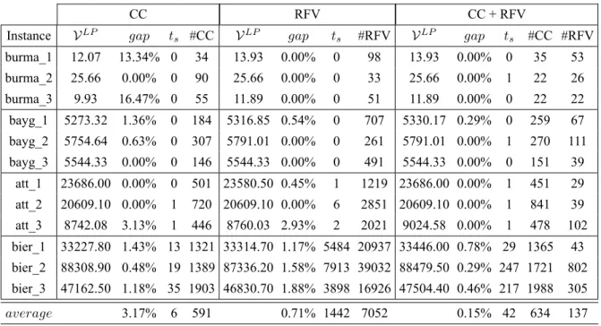
CC+RFV models. . . 95 5.7 Linear programming relaxation results for the instance set 1 with y- separation and
1-separation. . . 95 5.8 Linear programming relaxation results for instances a with y-separation and
1-separation. . . 96 5.9 Optimal values for the instance set 1 with y-separation and 1-separation. . . . 97 5.10 Optimal value for instances a with y-separation. . . . 98 5.11 Optimal value for instances a with 1-separation. . . . 98 5.12 Average LP relaxation results for the instance set 2. . . 99 5.13 Average gap and time by instance type for the instance set 2. . . 100 5.14 Optimal values for the instance set 2 with y-separation. . . 101 5.15 Statistics for the optimal value by instance type for the instance set 2. . . 104 5.16 Average LP relaxation results for the instance set 3. . . 105 5.17 Average gap and time by instance type for the instance set 3. . . 106 5.18 Optimal values for the instance set 3 with y-separation. . . 107 5.19 Statistics for the optimal value by instance type for the instance set 3. . . 110
5.22 Best upper bounds obtained with the B&C algorithm. . . 114
6.1 Best upper bounds for the benchmark instances obtained by Morán-Mirabal et al. (2014). . . 115 6.2 Experimenting parameter sets for the GA algorithm. . . 118 6.3 Experimenting generating individuals for the GA+NN algorithm. . . 119 6.4 Experimenting the LS algorithm. . . 121 6.5 Experimenting the LS_random algorithm. . . 122 6.6 Experimenting the LS_insertRemove algorithm. . . 123 6.7 Comparison of the different choosing criteria in the perturbation method. . . 127 6.8 Evaluation of the removal criterion Random_removal. . . 128 6.9 Combining both removal criteria using several ρ values. . . 129 6.10 Comparing different number of iterations in the ILS algorithm. . . 130 6.11 Optimal solution times for the variations of instance bier. . . 132 6.12 Comparing several values of r∗. . . 135 6.13 Comparing several values of ∆. . . 136 6.14 Comparing several values of Λ. . . 137 6.15 Results obtained with the hybrid algorithm. . . 138 6.16 Using the hybrid algorithm with dual information. . . 140 6.17 Summary of the best results obtained with the proposed heuristic algorithms. . . . 141 6.18 Summary of the final results obtained with the ILS algorithm. . . 143 6.19 Summary of the final results obtained with the hybrid algorithm. . . 144 6.20 Current best known upper bounds. . . 148
7.1 Average of linear programming relaxation results with the adapted models for the RFTSP. . . 163 7.2 Linear programming relaxation results for the instance set 1 with the inter- and
intrafamily formulations. . . 164 7.3 Linear programming relaxation results for the instance set 3 with the inter- and
intrafamily formulations. . . 165 7.4 Average of linear programming relaxation results with P-CC+RV model. . . 166 7.5 Average of linear programming relaxation results with y-separation. . . 167 7.6 Optimal values of the benchmark instances considering the RFTSP. . . 170
the RFTSP. . . 174 7.9 Optimal values of the instances from the instance set 3 considering the RFTSP. . . 175 7.10 Statistics for the optimal value by instance type for the instance set 3 considering
the RFTSP. . . 178 7.11 Optimal values of the instances from the instance set 4 considering the RFTSP. . . 179 7.12 Statistics for the optimal value by instance type for the instance set 4 considering
the RFTSP. . . 180 7.13 Best upper bounds found by the B&C algorithm for the RFTSP. . . 182 7.14 Reference values for the instance gr and pr considering the RFTSP. . . 187 7.15 Summary of the final results obtained with the ILS algorithm for the RFTSP. . . 187 7.16 Summary of the final results obtained with the hybrid algorithm for the RFTSP. . . 189 7.17 Current best known upper bounds for the RFTSP. . . 194
A.1 Complete description of the instance set 1. . . 207 A.2 Complete description of the instance set 2. . . 208 A.3 Complete description of the instance set 3. . . 212 A.4 Complete description of the instance set 4. . . 215
B.1 Linear programming relaxation results of the CC and RFV models without the heuristic separation algorithm. . . 218 B.2 Linear programming relaxation results of the CC+RFV model without the heuristic
separation. . . 219 B.3 Optimal values of the CC model without the heuristic callback. . . 220 B.4 Optimal values of the y-separation and the 1-separation without the heuristic callback.221 B.5 Linear programming relaxation results for instance set 2. . . 221 B.6 Optimal values for the instances of type high from the instance set 3 with 1-separation.224 B.7 Linear programming relaxation results for the instance set 3. . . 224 B.8 Linear programming relaxation results for instances rbg with SCF model. . . 228 B.9 Linear programming relaxation results for the instance set 4. . . 228
C.1 Results obtained with the GA algorithm. . . 232 C.2 Results obtained with the GA+NN algorithm. . . 232 C.3 Results obtained with the LS algorithm. . . 233 C.4 Results obtained with the LS_random algorithm. . . 234
C.7 Comparison of the choosing criteria M ean, M in and M ax. . . . 237 C.8 Comparison of the choosing criteria Random_choice and Least_chosen. . . 237 C.9 Results obtained with the removal criterion Random_removal. . . 238 C.10 Results obtained with the choosing criterion Random_choice and the combination
of both removal criteria with ρ = 200, ρ = 100 and ρ = 50. . . 239 C.11 Results obtained with the choosing criterion Random_choice and the combination
of both removal criteria with ρ = 25, ρ = 10 and ρ = 5. . . 239 C.12 Results obtained with the choosing criterion Least_chosen and the combination of
both removal criteria with ρ = 200, ρ = 100 and ρ = 50. . . 240 C.13 Results obtained with choosing criterion Least_chosen and the combination of
both removal criteria with ρ = 25, ρ = 10 and ρ = 5. . . 240 C.14 Results obtained performing 5000 iterations of the ILS algorithm. . . 241 C.15 Optimal results for the variations of instance bier. . . 242 C.16 Results obtained with the several r∗ values. . . 242 C.17 Results obtained with ∆ = 140, ∆ = 160 and ∆ = 200 values. . . 243 C.18 Results obtained with Λ = 30, Λ = 50 and Λ = 90 values. . . 244 C.19 Results obtained with the hybrid algorithm. . . 244 C.20 Results obtained with the hybrid algorithm with dual information. . . 245 C.21 Results obtained in five runs for the instances with unknown optimal value. . . 246
D.1 Linear programming relaxation results obtained with adapted formulations for in-stance set 1. . . 252 D.2 Linear programming relaxation results obtained with adapted formulations for
in-stance set 3. . . 252 D.3 Linear programming relaxation results obtained with the P-CC+RV model for the
instance set 1. . . 253 D.4 Linear programming relaxation results obtained with the P-CC+RV model for the
instance set 3. . . 254 D.5 Linear programming relaxation results obtained with the y-separation for the
in-stance set 1. . . 255 D.6 Linear programming relaxation results obtained with the y-separation for the
2.1 Cutting plane algorithm. . . 20 3.1 The neighborhood search procedure. . . 33 5.1 Separation algorithm for the CC inequalities. . . 77 5.2 Improved separation algorithm for the CC inequalities. . . 78 5.3 Heuristic separation of the CC inequalities. . . 80 5.4 Separation algorithm for the RFV inequalities. . . 82 5.5 Heuristic separation of the RFV inequalities. . . 83 5.6 Separation algorithm for the RFV inequalities for integer solutions. . . 84 5.7 Heuristic separation algorithm of both CC and RFV inequalities. . . 86 5.8 The y-separation algorithm. . . . 88 5.9 The 1-separation algorithm. . . 89 5.10 The local search procedure used in the heuristic callback. . . 93 6.1 The basic framework of the genetic algorithm. . . 118 6.2 The LS algorithm. . . 121 6.3 The basic framework of the ILS algorithm. . . 125 6.4 The local search procedure used in the ILS algorithm. . . 126 6.5 The perturbation method used in the ILS algorithm. . . 130 6.6 Constructive phase of the hybrid algorithm. . . 134 7.1 The local search procedure for the B&C algorithm for the RFTSP. . . 168 7.2 The local search procedure used in the ILS algorithm for the RFTSP. . . 184 7.3 The perturbation method used in the ILS algorithm for the RFTSP. . . 185 E.1 Separation algorithm for the subtour elimination constraints in the interfamily
sub-problem. . . 267 E.2 Separation algorithm for the P-CC inequalities. . . 269 E.3 Heuristic separation of the P-CC inequalities. . . 271 E.4 Separation algorithm for the P-RV inequalities. . . 273 E.5 Heuristic separation of the P-RV inequalities. . . 274
Introduction
Assume that products of the same type are scattered through different places in a warehouse and one must collect a given number of products of each type. This problem, the order picking problem in warehouses, motivated the family traveling salesman problem (FTSP), which will be addressed in this dissertation. More formally, consider a depot and a set of cities that is partitioned into several subsets, which are called families. The objective of the FTSP is to establish the minimum cost route that starts and ends at the depot and visits a given number of cities in each family.
The FTSP may be seen as a generalization of problems that have a wide variety of applications, which include the well-known traveling salesman problem and other variants. Additionally, the FTSP is a fairly recent problem and, in fact, as far as we know, there is only one article in the literature that addresses it. Therefore, for the reasons stated previously, the FTSP is a challenging problem to be studied within the scope of a Ph.D. dissertation.
The primary, and most general, objective of this dissertation is to study the FTSP in order to develop efficient methods that provide feasible solutions for this problem. The methods developed belong to one of two main categories: (i) exact methods, which guarantee that the solution obtained is the minimum cost feasible solution; and (ii) heuristic methods, which ensure that the solution obtained is feasible.
Regarding the exact methods, we will propose adaptations of methods from the literature de-veloped for other problems, namely for the traveling salesman problem, and we will also develop new methods that take into account the specificities of the FTSP. The proposed methods will not only be compared theoretically but also empirically by using a small subset of test instances. The method that provides the best results is applied to all the test instances.
The heuristic methods are used to address the instances which the exact methods could not solve efficiently. Similarly to what was done for the exact methods, we use a small subset of test instances to do the parameter tuning of the several heuristic methods and to evaluate their behavior. The
heuristic method that provides the solutions with the lowest cost will be used to solve the instances that the exact methods were unable to.
As a complement to this dissertation we decided to create a variant of the FTSP, which seems to be a natural variant and that arises by imposing the condition that cities from the same family must be visited consecutively. We denote this variant by the restricted family traveling salesman problem (RFTSP). We will adapt for the RFTSP the methods, both exact and heuristic, that provided the best results for the FTSP. Additionally, we developed an exact method that can only be applied to the RFTSP, which is compared to the adapted exact method through computational testing.
Finally, we created a website devoted to the FTSP which gathers the test instances used in this dissertation, both from the literature and the generated ones, and the best results obtained so far, which are either exact results or heuristic results. The site also contains the same type of information for the RFTSP.
This dissertation is organized as follows. In Chapter 2 we introduce definitions and theoretical results that will be used during this dissertation. Therefore, this chapter is purely expository and it is independent of the FTSP.
In Chapter 3 we provide a formal definition for the FTSP and present the notation used during the remainder of the dissertation. Additionally, we present the literature review as well as some problems that under specific circumstances can be solved as the FTSP. Some basic constructive heuristics are also described. We conclude this chapter by describing the FTSP instance generator developed and by presenting the test instances used.
Chapter 4 is devoted to the exact methods. We start by presenting several exact methods and then, by using a small subset of test instances, we establish a theoretical and an empirical comparison between the exact methods proposed.
In Chapter 5 we present the branch-and-cut algorithm, which is an algorithm used to solve some of the exact methods proposed, and the computational results obtained for the test instances with the best exact method.
In Chapter 6 we present the heuristic methods proposed for the FTSP, establish an empirical comparison between them, by using a small subset of test instances, and carry out the computational experiment, which consists in applying the best heuristic method to the instances that the exact methods could not solve efficiently.
Chapter 7 is devoted to the RFTSP, the variant of the FTSP that we proposed. We present exact methods for the RFTSP which are either adaptations of the exact methods for the FTSP or methods developed specifically for the RFTSP and we establish an empirical comparison between the exact methods proposed. We also develop heuristic methods by adapting the heuristic methods for the
FTSP. Finally, we present the computational experiment for the RFTSP.
We conclude this dissertation in Chapter 8 where we draw the main conclusions from this work and provide some bullet points of what the future work could entail.
Mathematical Background
The purpose of this chapter is to present or clarify some definitions and theoretical results that are going to be used throughout this dissertation. Therefore, this chapter is purely expository as the results presented are a collection of results from the literature. This chapter is divided into five sections: graph theory, polyhedral theory, linear programming theory, complexity theory and, fi-nally, some basic linear programming problems. More precisely, in Section 2.1 we present concepts related to graph theory, concepts related to polyhedral theory are presented in Section 2.2, in Sec-tion 2.3 we address linear programming theory, complexity theory is presented in SecSec-tion 2.4 and, finally, in Section 2.5 we present some basic linear programming problems.
2.1
Graph theory
One seminal paper addressing graph theory dates back to 1739 and it was published by Euler. Since then graphs have been used to model a wide variety of problems, being routing one of the most common type. Information related to graph theory can be found in Christofides (1975) and Ahuja et al. (1993), for example.
A graph G = (N, A) is defined as a pair of sets in which N = {1, 2, . . . , n} is a non-empty finite set called node (or vertice) set and A = {a1, a2, . . . , am} is either an arc set in which its
elements are pairs of elements of N or an edge set, that is, a set of subsets with two elements of N . In the former case, there is an orientation assigned to the elements of A and in the latter case, there is no orientation assigned to the elements of A. If A is an arc set, then G is called a directed graph whereas if A is an edge set, then G is called a nondirected graph.
Example 1. Figure 2.1 shows examples of a directed graph (Figure 2.1a) and a nondirected graph
1 2
3 4
(a) Directed graph.
1 2
3 4
(b) Nondirected graph. Figure 2.1: Examples of a directed and a nondirected graph.
We assume that G is a directed graph since any nondirected graph may be equivalently repre-sented as a directed graph by assigning two arcs to each edge. We represent an arc ai as a pair of
nodes, that is, ai = (j, k) where j is the initial node and k is the final node of the arc. Additionally,
if there is an arc between j and k we say that j and k are adjacent nodes. We also consider that G is a simple graph, that is, G contains a maximum of one arc between each pair of nodes and does not contain arcs which have the same initial and final nodes.
Example 2. To illustrate the definitions presented throughout this section consider the Ge graph presented in Figure 2.2. 1 2 3 4 5 6
Figure 2.2: Example of a directed and simple graph.
Given a graph G = (N, A), a subgraph Gs = (N
s, As) is a graph such that Ns⊆ N and As =
{(i, j) ∈ A : i, j ∈ Ns}. A path (chain in a nondirected graph) is a sequence of arcs such that the
final node of one arc is the initial node of the following one, that is,{(i1, i2), (i2, i3), . . . , (ik−1, ik)}.
Node i1 is the initial node of the path and node ikis the final node of the path. A circuit (cycle in a
nondirected graph) is a path in which the initial and the final nodes are the same, that is, i1 = ik.
Example 3. An example of a path in Ge is {(1, 2), (2, 3), (3, 4)} and an example of a circuit is
A simple path (or circuit) is a path (or circuit) which does not use the same arc more than once and an elementary path (or circuit) is a path (or circuit) that does not use the same node more than once.
Example 4. The path in Gepresented in Example 3 is a simple and elementary path. However, the path{(1, 2), (2, 3), (3, 5), (5, 2), (2, 3)} in Geis neither simple (it repeats arc (2, 3)) nor elementary
(it repeats nodes 2 and 3).
An elementary circuit (or path) that goes through every node of the graph is a Hamiltonian circuit (or path) and a simple circuit (or path) that traverses every arc of the graph is an Eulerian circuit (or path). A graph is Hamiltonian if it contains a Hamiltonian circuit and is Eulerian if it contains an Eulerian circuit.
Example 5. As the circuit presented in Example 3 is the only existing circuit in Gewe can conclude
that Ge is neither Hamiltonian (the circuit does not contain each node exactly once) nor Eulerian
(the circuit does not contain each arc exactly once).
The number of arcs that have node i as their initial node is called outdegree of node i. Equiva-lently, the number of arcs that have node i as their final node is designated as the indegree of node
i.
Example 6. Considering graph Ge, the outdegree of node 2 is 1 while the indegree of node 2 is 2.
A graph G = (N, A) is complete if for every i, j ∈ N, i ̸= j there exists the arcs (i, j) and (j, i).
Example 7. Graph Geis not complete since, for instance, the arc (6, 1) does not exist.
We say that two nodes i and j are connected if, ignoring the orientation of the arcs, there is at least one chain from i to j. A graph is connected if every pair of nodes in N is connected, otherwise the graph is disconnected. If there is a path between every pair of nodes then the graph is strongly
connected. A disconnected graph is comprised of several connected subgraphs which are called components.
Example 8. Graph Ge is connected but it is not strongly connected as there is no path between
nodes 6 and 4. If we remove the arc (1, 2), then the resulting graph is a disconnected graph with two components. One component is the subgraph with the node set{1, 6}, and the other component is the subgraph with the node set{2, 3, 4, 5}.
A cut is a partition of the node set N into two disjoint subsets S and S′ = N \ S. Each cut defines a cut-set [S′, S] which is a set of arcs (i, j) ∈ A such that i ∈ S′ and j ∈ S or i ∈ S and
j ∈ S′. An s-t cut is a cut-set [S′, S] that is defined with respect to two distinct nodes s and t, such
that: s∈ S′ and t∈ S.
Example 9. Considering the graph Geand S ={1}, we have [S′, S] ={(1, 2), (1, 6)}, which is an
s-t cut if, for instance, s = 1 and t = 2 however, if s = 2 and t = 6 the cut [S′, S] is not an s-t cut.
It is possible to associate a value cijwith each arc (i, j) ∈ A, which are called costs and the cost
of a generic path Π is defined as∑(i,j)∈Πcij. A graph is symmetric if the cost matrix associated
with A is symmetric, that is, if cij = cji,∀(i, j) ∈ A, and asymmetric if there exists at least a pair
of nodes such that cij ̸= cji, with (i, j)∈ A.
2.2
Polyhedral theory
In this section we present a summary of definitions and results addressing polyhedra, which are defined later on. For more on polyhedral theory see Nemhauser and Wolsey (1988), Wolsey (1998), Schrijver (1998) and Conforti et al. (2014).
Definition 1. A vector y ∈ Rn is a linear combination of vectors x1, x2, . . . , xk ∈ Rn if y =
∑k
i=1λixi, with λ1, λ2, . . . , λk ∈ R.
Definition 2. A vector y ∈ Rn is an affine combination of vectors x1, x2, . . . , xk ∈ Rn if it is a linear combination and∑ki=1λi = 1, with λ1, λ2, . . . , λk ∈ R.
Definition 3. A vector y ∈ Rn is a convex combination of vectors x1, x2, . . . , xk ∈ Rn if it is a
linear combination and∑ki=1λi = 1, with λ1, λ2, . . . , λk ≥ 0.
Definition 4. The convex hull of a set X ∈ Rn, denoted by conv(X), is the set of all vectors (or points) that are convex combinations of the vectors (or points) in X.
Definition 5. A set of vectors x1, x2, . . . , xk ∈ Rn is linearly independent if the only solution of the system∑ki=1λixi = 0n, with λi ∈ R, is λi = 0,∀i = 1, . . . , k.
The maximum number of linearly independent points inRnis n.
Definition 6. A set of vectors x1, x2, . . . , xk ∈ Rn is affinely independent if the only solution of
the system∑ki=0λixi = 0n,
∑k
Note that if vectors x1, x2, . . . , xk ∈ Rn are linearly independent then they are also affinely
independent. However, the reciprocal is not valid. Consequently, the maximum number of affinely independent points inRnis n + 1 (n linearly independent points and the zero vector).
We define matrices D∈ Rm×n, with m rows and n columns, and b∈ Rm×1, with m rows and 1 column. Note that the rows of D may be seen as vectors di
R∈ Rn, ∀i = 1, . . . , m, and equivalently,
the columns of D may be viewed as vectors di
C ∈ Rm, ∀i = 1, . . . , n.
Definition 7. The maximum number of linearly independent rows in D is the rank of D and is
denoted by rank(D).
Example 10. Consider the following matrix De ∈ R3×2:
De = 1 1 0 2 1 2
The vectors (1, 1), (0, 2), (1, 2), which correspond to the rows of matrix De, are not linearly
independent since (1, 2) = 1 × (1, 1) + 12 × (0, 2) but vectors (1, 1) and (0, 2) are. Therefore,
rank(De) = 2.
Considering the vector x∈ Rn×1 and the matrices D and b presented previously, it is possible
to define a system of linear inequalities Dx≤ b. We define (D=, b=) as the submatrix of (D, b) that
contains the rows associated with the equalities present in the system and (D≤, b≤) as the submatrix associated with the inequalities.
Definition 8. A polyhedron P ⊆ Rn is the set of points that satisfies a finite number of linear
inequalities, that is, P ={x ∈ Rn: Dx≤ b}, with D ∈ Rm×nand b∈ Rm×1. A polytope P ⊂ Rn
is a polyhedron that is bounded, that is, P ⊆ {x ∈ Rn : −ω ≤ x
j ≤ ω, with ω > 0, ∀j ∈
{1, . . . , n}}.
Throughout this dissertation we will focus our study on bounded polyhedra since it is always possible to define an M ∈ N such that 0 ≤ x ≤ M. Consequently, henceforth we assume that
P = {x ∈ Rn : Dx≤ b} is a polytope.
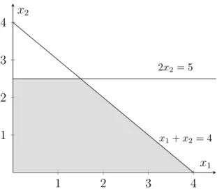
Example 11. Figure 2.3 shows the graphical representation of the polytope Pe = {x ∈ R2 :
x1 + x2 ≤ 4, 2x2 ≤ 5, 13x1 + x2 = 3, x1, x2 ≥ 0} in light gray. Polytope Pe will be used to
1 2 3 4 1 2 3 4 x1+ x2= 4 2x2= 5 1 3x1+ x2= 3 x1 x2
Figure 2.3: Graphical representation of the Pepolytope.
Definition 9. A polyhedron P is of dimension k, denoted by dim(P ) = k, if the maximum number
of affinely independent points in P is k + 1.
Example 12. The polytope Pehas at least three affinely independent points: (0, 0), (1, 0) and (0, 1). Therefore, we can deduce that dim(Pe)≥ 3 − 1 = 2. As we saw previously, the maximum number
of affinely independent points inR2is 3 so, in this case, we can ensure that the equality dim(Pe) = 2
holds. However, usually that is not possible hence the importance of the next proposition.
Proposition 1. If P ⊆ Rn, then dim(P ) + rank(D=, b=) = n.
Example 13. Polytope Pe ⊆ R2 therefore dim(Pe) = 2− rank(D=e, b=e). As Peis not defined by
any equality, then rank(D=
e, b=e) = 0. Consequently, dim(Pe) = 2.
Definition 10. Given π ∈ R1×nand π0 ∈ R, an inequality πx ≤ π0is a valid inequality for P ⊆ Rn
if is satisfied by all x∈ P .
A given valid inequality πx ≤ π0 is violated by a point y if y does not satisfy that inequality,
that is, πy > π0.
Definition 11. Consider πx≤ π0 and µx≤ µ0 two distinct valid inequalities for P ⊆ Rn. We say
that πx ≤ π0 dominates µx ≤ µ0 if there exists u∈ R : u > 0 such that π ≥ uµ, π0 ≤ uµ0 and
(π, π0)̸= (uµ, uµ0).
Definition 12. A valid inequality πx ≤ π0 is redundant in the description of P ⊆ Rnif there are
k ≥ 2 valid inequalities µix≤ µi
0, with i = 1, . . . , k, for P and weights ui > 0, with i = 1, . . . , k,
such that (∑ki=1uiµi)x≤
∑k i=1uiµ
i
Example 14. Inequality x2 ≤ 3 is a valid inequality for Pe, while inequality x1 ≤ 3 is not since
(4, 0)∈ Peand (4, 0) does not satisfy the previous inequality (x1 = 4 ≰ 3). Additionally, inequality
x2 ≤ 3 is dominated by inequality 2x2 ≤ 5 ⇔ x2 ≤ 52 as 52 < 3. We can also verify that inequality 1
3x1 + x2 ≤ 3, which is a valid inequality for Pe, is redundant since it can be obtained as a linear
combination of inequalities x1+ x2 ≤ 4 and 2x2 ≤ 5, with u1 = u2 = 13.
Definition 13. Let πx ≤ π0 be a valid inequality for P and F = {x ∈ P : πx = π0}. Then F is
called a face of P and we say that πx ≤ π0 represents F . A face F is a proper face if F ̸= ∅ and
F ̸= P .
Example 15. The following sets are faces of the polytope Pe:
• F0 ={(x1, x2)∈ Pe : x2 = 3};
• F1 ={(x1, x2)∈ Pe : x1+ x2 = 4};
• F2 ={(x1, x2)∈ Pe : 2x2 = 5}, and;
• F3 ={(x1, x2)∈ Pe : 13x1+ x2 = 3}.
The only face that is not a proper face of Peis F0, since F0 =∅.
Definition 14. A face F of P is a facet of P if dim(F ) = dim(P )− 1.
Proposition 2. Every inequality dkRx≤ bk from the system Dx≤ b that represents a face of P of
dimension less than dim(P )− 1 is irrelevant to the description of P .
Example 16. Since F1, F2 and F3 are faces of Pe we know that dim(Fi) ≤ dim(Pe)− 1 = 1,
∀i = 1, 2, 3 (faces have one additional equality). Points (4, 0) and (3 2,
5
2) belong to F1 and are
affinely independent, therefore dim(F1) ≥ 2 − 1 ⇒ dim(F1) = 1, thus F1 is a facet of Pe. By
using the same argument for face F2and the points (0,52) and (32,52) we can conclude that F2is also
a facet of Pe. Finally, face F3 ={(32,52)}, thus dim(F3) = 1− 1 = 0. Another way of proving that
the inequality 13x1+ x2 = 3 is redundant in the description of Peis by using Proposition 2. As F3
is not a facet, it is irrelevant in the description of Pe.
Henceforth we assume that the polytope Peis defined by the non-redundant inequalities, that is,
1 2 3 4 1 2 3 4 x1+ x2= 4 2x2= 5 x1 x2
Figure 2.4: Graphical representation of the Pepolytope without the redundant inequalities.
Definition 15. A point x∈ P is an extreme point of P if it cannot be obtained as a convex
combi-nations of other points in P .
Proposition 3. A point x ∈ P is an extreme point of P if and only if x is a zero-dimensional face
of P .
Example 17. As we saw previously dim(F3) = 0, therefore F3 ={(32,52)} is an extreme point of
Pe.
Definition 16. Given a polyhedron P ⊆ Rn−p× Rp, the projection of P onto the subspaceRn−p, denoted projxP , is defined as:
projxP ={x ∈ Rn−p : (x, w)∈ P for some w ∈ Rp}
Example 18. The polytope Pe ⊆ R2may be seen as a subset ofR1×R1, thus it is possible to project
Peonto the space of x1and onto the space of x2. For example, by projecting Peonto the subspace
of x1, we obtain projx1Pe ={x1 ∈ R : (x1, x2) ∈ Pefor some x2 ∈ R} and, by observing Figure
2.4 we can conclude that projx1Pe = [0, 4]. Analogously, projx2Pe= [0,
2 5].
2.3
Linear programming theory
Linear programming is a mathematical field devoted to the study of problems involving linear func-tions. Books that address linear programming theory are, for instance, Nemhauser and Wolsey (1988), Wolsey (1998) and Schrijver (1998).
Let D ∈ Rm×n, b ∈ Rm×1 and c ∈ R1×n be matrices with known values and x ∈ Rn×1 be
the vector of variables. A linear programming (LP) problem consists in determining the value of the variables, in this case the x values, that minimize (or maximize) a linear function cx, which is called objective function, over a polyhedron, that is,
min{cx : Dx ≤ b, x ≥ 0n×1}.
Each inequality of the system Dx ≤ b is called a constraint of the problem and the inequalities
x≥ 0n×1are called the domain constraints of variables x.
When we impose the additional condition that some of the variables must be integer, that is,
x1, . . . , xk ∈ Z, with k < n, we obtain a mixed integer linear programming problem. When all
variables must be integer (i.e., k = n) we have an integer linear programming (ILP) problem. A particular case of ILP problems arises when the variables are binary, that is, x ∈ {0, 1}n×1. This particular case is called binary linear programming.
Definition 17. A polyhedron P ⊆ Rn is a formulation for a set X ⊆ Zn−p × Rp if and only if
X = P ∩ (Zn−p× Rp).
Consider the following LP problem: min{cx : x ∈ P }. An element x ∈ P is called a feasible
solution for that LP problem. If P =∅ we say that the problem is unfeasible. The element x∗ ∈ P
such that cx∗ ≤ cx, ∀x ∈ P is an optimal solution of the LP problem and cx∗ is the optimal value. Note that the optimal solution of an LP problem is not necessarily unique. Additionally, recall that we are particularly interested in bounded polyhedra, that is, polytopes.
Theorem 1. Consider a polytope P ∈ Rnand the linear programming problem min{cx : x ∈ P }.
If P ̸= ∅, then there is an optimal solution of the linear programming problem that is an extreme point of P .
According to Theorem 1, when P is a polytope, it is possible to find the optimal solution of an LP problem by enumerating all of its extreme points, however, this is not viable in practice since, usually, there are too many extreme points. Nowadays, the common approach to solve LP problems is by using commercial solvers that have specific algorithms implemented. This is how we will solve LP problems throughout this dissertation.
Example 19. Let Pe be the polytope presented in Section 2.2. Consider the following LP and ILP problems, with the same formulation Pe:
max{x1+ 3x2 : x∈ Pe}
which we will designate by LPe and Pe, respectively. Note that we called the ILP problem by the
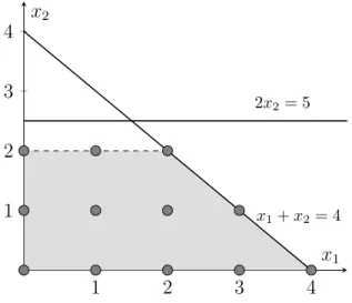
same name as the formulation since this is the notation adopted in the remainder of the dissertation. Figure 2.4 shows the set of feasible solutions for the LPeproblem while Figure 2.5 shows the
set of feasible solutions for the Peproblem. By comparing both figures we can see how adding the
integrality condition changes the solution set. In fact, the solution set of Peis not even a polyhedron.
1 2 3 4 1 2 3 4 x1+ x2= 4 2x2= 5 x1 x2
Figure 2.5: Graphical representation of the set of feasible solutions for the Peproblem.
We now analyze the optimal solutions of the LPeand the Peproblems presented previously. In
the case of the LPeproblem, the optimal solution is (32,52) and the optimal value is 32 + 3× 52 = 9,
whilst for the Pe problem, the optimal solution is (2, 2) and the optimal value is 2 + 3× 2 = 8.
Note that the optimal solution of the LPeproblem corresponds to an extreme point of the polytope
Pe, which was determined in Section 2.2, while the optimal solution of the Pe problem does not
correspond to any extreme point of the polytope Pe. Nevertheless, if we were to consider the convex
hull (see Definition 4 in Section 2.2) of the points which are feasible solutions for the Peproblem,
then its optimal solution would be an extreme point. This fact shows the importance of the convex hull.
Proposition 4. For any X ⊆ Rnconv(X) is a polyhedron.
Proposition 5. For any X ⊆ Rnthe extreme points of conv(X) all belong to X.
From the results presented previously, in Propositions 4 and 5, we can conclude that the LP problem min{cx : x ∈ X} is equivalent to the LP problem min{cx : x ∈ conv(X)}. In particular, solving the ILP problem min{cx : x ∈ X, x ∈ Zn} is equivalent to solving the LP
Example 20. Figure 2.6 shows, in light gray, the convex hull of the points which are feasible
solutions of the Peproblem.
1 2 3 4 1 2 3 4 x1+ x2= 4 2x2= 5 x1 x2
Figure 2.6: Graphical representation of the convex hull of the set of feasible solutions of the Peproblem.
When developing a formulation for an ILP problem, the aim is to create a system of inequalities that defines the convex hull of points that are the feasible solutions of the ILP problem. In most cases this is a hard task, thus, the formulation developed should give a close approximation of the convex hull.
Example 21. By observing Figure 2.6, we verify that the half-space defined by the dashed line
gives a better approximation of the convex hull of the points that are feasible solutions of the Pe
problem than the half-space 2x2 ≤ 5, thus it is better to include in the formulation the inequality
that originates the half-space represented by the dashed line than the inequality 2x2 ≤ 5.
Definition 18. Given a set X ⊆ Rnand two formulations P1and P2for X, P1is a better formulation
than P2 if P1 ⊆ P2.
Definition 19. Given a set X ⊆ Rnand two formulations P1and P2 for X, P1 is not comparable
to P2 if P1\ P2 ̸= ∅ and P2\ P1 ̸= ∅.
In practice, in order to show that two formulations P1 and P2 are not comparable we consider
two points x1 ∈ P1 and x2 ∈ P2and verify that x1 ∈ P/ 2and x2 ∈ P/ 1.
Definition 20. For the ILP min{cx : x ∈ P ∩ Zn} with formulation P = {x ∈ Rn : Dx ≤
b, x ≥ 0n×1}, the linear programming relaxation is the linear program min{cx : x ∈ P }.
Example 22. Note that the LPe problem, presented in Example 19, is the linear programming relaxation of the Pe problem, also presented in Example 19, as the LP relaxation is obtained by
relaxing the integrality conditions of the ILP problem. Consequently, the LPe problem will be
called LP relaxation of the Peproblem henceforth.
Proposition 6. Suppose that P1 and P2 are two formulations for the problem min {cx : x ∈
X ⊂ Zn} such that P
1 is a better formulation than P2. Let VLP(Pi) be the linear programming
relaxation value of min{cx : x ∈ Pi ⊂ Zn}, with i = 1, 2, then VLP(P1)≥ VLP(P2) for all c.
If P1 and P2are two not comparable formulations for the set X ⊂ Rn, then it is not possible to
establish a relationship between their linear programming relaxation values which is valid for every cost matrix c ∈ R1×n.
Example 23. Consider a new LP problem with the formulation Pconv = conv(Pe∩ Z2), that is,
max{x1+ 3x2 : x∈ Pconv},
which will be designated as the LP relaxation of the Pconv. Note that the formulation Pconv is the
one represented in Figure 2.6. Since the formulation Pconv is contained in the formulation Pe and
due to the result of Proposition 6, we expect thatVLP(Pconv)≤ VLP(Pe). In fact,VLP(Pconv) = 8
andVLP(Pe) = 9.
Definition 21. A formulation P ⊂ Rn is an ideal formulation for a set X ⊂ Zn if and only if
P = conv(X).
Example 24. Formulation Pconv is an ideal formulation as it corresponds to convex hull of the set
of points that are feasible solutions of the Pe problem, as mentioned previously. A consequence
of having an ideal formulation is that when we solve an LP problem over conv(Pe) the optimal
solution obtained is integer, and, therefore, it is the optimal solution of the ILP problem.
Considering the matrices D, b and c defined as previously, we define a formulation P ={x ∈ Rn : Dx ≤ b, x ≥ 0n×1} for the ILP min{cx : x ∈ X = P ∩ Zn}. To simplify, we will
refer to the ILP as P , which is the name of the formulation. When the formulation P is not ideal, that is, conv(X)̸= P , we have to resort to a branch-and-bound algorithm to determine the optimal solution of the ILP problem. The basic idea of a branch-and-bound (B&B) algorithm is to partition the set of feasible solutions of P into smaller and easier to search subsets. We start by solving the LP relaxation of P . Since we are considering a minimization problem,VLP(P ) is a lower bound
for the optimal value of P . Similarly, the value of any feasible solution for P is an upper bound for its optimal value. Let x0 be the optimal solution of the LP relaxation of P . If x0 is integer,
then it corresponds to the optimal solution of P , otherwise we must do branching on a variable with fractional value. Let xi
B&B subproblems, Pk1 and Pk2, which correspond to the problem P with the additional constraints xi ≤ ⌊xi
0⌋ and xi ≥ ⌈xi0⌉, respectively (other branching techniques may be used, see for instance
Barnhart et al., 1998). The B&B subproblems Pk1and Pk2are added to thelist of open subproblems.
Then, we choose and remove a B&B subproblem Pk from the list of open subproblems and solve
its LP relaxation. If Pk is not unfeasible, letVLP(Pk) be the LP relaxation value of Pk and xk be
the corresponding optimal solution. If xkis feasible for P , that is, if it is integer, we verify whether
or notVLP(P
k) is lower than the best upper bound found so far during the B&B algorithm, which
we designate by U B∗, and, if it is, we update U B∗ to VLP(P
k). Otherwise, that is, if xk is not
feasible for P , we also must check whether VLP(Pk) < U B∗ or not. IfVLP(Pk) ≥ UB∗, then
there is no need to do branching on the optimal solution of the LP relaxation of Pk as the B&B
subproblems that stem from Pk would never originate a solution with a lower value than U B∗. If
VLP(P
k) < U B∗, we do branching on a variable with a fractional value as we explained previously
and the B&B subproblems originated go to the list of open subproblems. The B&B algorithm stops when the list of open problems is empty and one optimal solution corresponds to the integer solution with value U B∗.
Having formulations that provide a high LP relaxation value (in the case of minimization prob-lems) is very important in order to have an efficient B&B algorithm, since we can eliminate B&B subproblems if their LP relaxation value is higher than the best upper bound found so far. We can create several formulations for the same ILP problem, namely by using different variables and, consequently, defined in different subspaces. In these cases in order to compare formulations we must use projections so that all formulations are defined in the same subspace. Additionally, we can also create formulations with an exponential number of constraints (or variables), which are called
non-compact formulations. Formulations with a polynomial number of constraints (or variables)
are designated by compact formulations.
Linear duality
Given matrices D ∈ Rm×n, b ∈ Rm×1 and c ∈ R1×n and the vector of variables x ∈ Rn×1, we define the primal problem (P) as the following linear programming problem:
max{cx : Dx ≤ b, x ≥ 0n×1} The dual problem (D) associated with (P) is the LP problem:
min{uTb : DTu≥ cT, u≥ 0m×1}
Note that the dual problem of the LP problem (D) is the LP problem (P). Therefore, it is equivalent to define the maximization problem as the primal problem and the minimization problem as the dual problem or vice-versa.
Proposition 7 (Weak duality). Consider the primal problem (P) and the dual problem (D) defined
previously and let x and u be feasible solutions for (P) and (D), respectively. Then, cx ≤ uTb.
A consequence from Proposition 7 is that any feasible solution of (D) provides an upper bound for the optimal value of (P).
Proposition 8. Let x∗and u∗be feasible solutions for (P) and (D), respectively. Then the following statements are equivalent:
(i) x∗ and u∗ are, respectively, the optimal solutions of (P) and (D). (ii) cx∗ = (u∗)Tb.
(iii) If a component of u∗ is positive, the corresponding inequality in Dx ≤ b is satisfied by x∗ with equality, that is, (u∗)T(b − Dx∗) = 0, and, equivalently, if a component of x∗ is
positive, the corresponding inequality in DTu ≥ cT is satisfied by u∗ with equality, that is,
x∗(DTu∗− cT) = 0.
Example 25. Consider the formulation Pdual ={(u1, u2)∈ R2 : u1 + 2u2 ≥ 3, u1 ≥ 1, u1, u2 ≥
0}, which is represented in Figure 2.7, and the following LP problem, which we designate by LPdual:
w = min{4u1+ 5u2 : (u1, u2)∈ Pdual}.
Notice that, the LPdual problem is the dual problem associated with the LP relaxation of the
Pe problem. The optimal solution of the LPdual problem is (1, 1) and the optimal value is w =
4× 1 + 5 × 1 = 9, which corresponds to the optimal value of the LP relaxation of the Peproblem.
Consider now the ILP problem Pe, the only relationship that we can establish between the LPdual
and the Pe problems is given by Proposition 7, that is, the value of any feasible solution of the
LPdual problem is greater than or equal to the value of any feasible solution of the Pe problem. In
1 2 3 4 1 2 3 4 u1+ 2u2= 3 u1= 1 u1 u2
Figure 2.7: Graphical representation of the formulation Pdual.
Generating valid inequalities
Consider X = P ∩ Zn, with P = {x ∈ Rn : Dx ≤ b, x ≥ 0n×1}. We know that is possible
to formulate any ILP problem as an LP problem by using its convex hull. However, in order to do so we would need to have an explicit description of conv(X). Therefore, we must find valid inequalities for conv(X) that are violated by the points in P \ conv(X). We present several ways of generating valid inequalities.
space
Chvátal-Gomory procedure to construct valid inequalities for X: Recall that di
C, with i =
1, . . . , n, are the column vectors of D and let λ∈ Rm×1, λ
j ≥ 0, with j = 1, . . . , m :
(i) the inequality∑ni=1(λdi
C)xi ≤ λb is valid for P ;
(ii) the inequality∑ni=1⌊λdi
C⌋xi ≤ λb is valid for P ; and
(iii) the inequality∑ni=1⌊λdiC⌋xi ≤ ⌊λb⌋ is valid for X.
Theorem 2. Every valid inequality for X can be obtained by applying the Chavátal-Gomory
pro-cedure a finite number of times.
Example 26. Recall the inequality 2x2 ≤ 5 used in formulation Pe. By using the procedure (iii) of
the Chvátal-Gomory procedure to construct valid inequalities we obtain the inequality x2 ≤ ⌊52⌋ = 2
which, according to Theorem 2, is a valid inequality for the set of points which corresponds to the feasible solutions of the Pe problem. In fact, this is the inequality that defines the half-space
represented by a dashed line in Figure 2.6 and describes the convex hull of the set of points which are feasible solutions of the Peproblem.