M
ASTER OF
S
CIENCE IN
M
ONETARY AND
F
INANCIAL
E
CONOMICS
M
ASTER
F
INAL
W
ORK
D
ISSERTATION
What Is the Size and Cyclicality of Mark-ups in
Portuguese Industries?
ANDRÉ FILIPE FIGUEIREDO SILVA
M
ASTER OF
S
CIENCE IN
M
ONETARY AND
F
INANCIAL
E
CONOMICS
M
ASTER
F
INAL
W
ORK
D
ISSERTATION
What Is the Size and Cyclicality of Mark-ups in
Portuguese Industries?
André Filipe Figueiredo Silva
Supervisor:
Luís Filipe Pereira da Costa
Carlos Daniel Rodrigues Ascenção Santos
i
Abstract
This dissertation provides new insights on the estimation of mark-up ratios in Portugal, using annual panel data for Portuguese manufacturing industries over the period 2004-2010. I used a production-function approach for single-product firms and made weak assumptions on the productivity stochastic process. The main difference from this empirical setting is that I used product-level quantity and price information, rather than firm-level revenues. The conclusion rests on the finding that mark-up ratios or price-marginal cost ratios, are significantly larger than one in general, i.e. prices tend to be larger than marginal costs. This study also contributes for the discussion on the cyclicality of mark-ups and provides evidence that they tend to be countercyclical with GDP.
KEYWORDS: Mark-ups, Productivity, Production Function. JEL CODES: C23, C36, D24, D43, E32, L22
ii
C
ONTENTS1! Introduction ... 1!
2! Literature ... 3!
2.1! Measuring Market Power ... 3!
2.2! Estimating Production Functions ... 7!
3! Methodology ... 8!
4! Data description ... 13!
5! Empirical Analysis ... 16!
5.1! Interpretation and Possible Estimation Biases ... 16!
5.2! Interpreting Mark-ups ... 20!
5.3! Comparison with previous studies ... 23!
5.4! Mark-up and TFP distributions ... 24!
6! Cyclicality with GDP ... 27!
7! Conclusion ... 31!
References ... 33!
iii
A.1! Sample Selection ... 36!
A.2! Construction of Physical Stock of Capital ... 39!
B.1! OLS Results and Figures ... 39!
B.2! GMM Coefficients ... 45!
B.3! GMM Results ... 46!
B.4! Indicators of median mark-up level ... 47!
iv
TABLE I Sample Size of Firms per Industry and Year ... 16!
TABLE II GMM Estimates for the Coefficients of the Production Function ... 17!
TABLE III Returns to Scale Test at 1 per cent significance ... 18!
TABLE IV Validity of the Instruments ... 19!
TABLE V Mark-up Regression with GDP: Estimated Values in eq. (12) ... 28!
TABLE VI Mark-up regressions: Estimated Values in eq. (13) ... 29!
TABLE VII Number of firms per year for the IES database ... 36!
TABLE VIII Number of products and firms per year for the IAPI database ... 36!
TABLE IX Number of firms by number of products reported (IAPI database) ... 36!
TABLE X Number of firms per year for total sample ... 37!
TABLE XI Number of firms per year per industry from the IAPI database, merged and usable sample ... 37!
TABLE XII Single-product firms versus multi-product firms - summary statistics ... 38!
TABLE XIII OLS Estimations for quantities: Median mark-up obtained using the labour share without intermediate inputs ... 39!
TABLE XIV OLS Estimations for Value Added: Median Mark-up obtained using the labour share without intermediate inputs ... 40!
TABLE XV OLS Estimations for Revenues: Median mark-up obtained using the labour share without intermediate inputs ... 40!
TABLE XVI OLS Estimations for Quantities: Median mark-up obtained using both labour and intermediate inputs shares ... 41!
TABLE XVII OLS Estimations for Value Added: Median Mark-up obtained using both labour and intermediate inputs shares ... 41!
v
TABLE XVIII OLS Estimations for Revenues: Median mark-up obtained using both labour and intermediate inputs shares ... 42! TABLE XIX Coefficients of GMM Estimation ... 45! TABLE XX GMM Estimations Median mark-up: obtained using the labour share ... 46! TABLE XXI GMM Estimations: Median mark-up obtained using the labour share (without intermediate inputs) ... 46! TABLE XXII GMM Estimations: Median Mark-up obtained by Labour and
Intermediate Inputs share ... 47! TABLE XXIII Correlation between log of output and mark-up level per industry ... 47! TABLE XXIV Intensity and correlation between the log of physical stock of capital and median mark-up level ... 48! TABLE XXV Kolmogrov-Smirnov Normality Test for Mark-up ... 48! TABLE XXVI Unit root test for TFP and Mark-up ... 49!
vi
Acknowledgments
Firstly, I would like to thank Professor Luís Costa who gave me support and motivation to proceed with my dissertation. The knowledge and the patience he had with me were crucial to cope with all of this hard process. I would also like to thank Professor Carlos Santos for the support. It has been a privilege to work with both.
The dissertation was made as part of project PTDC/EGE-ECO/104659/2008, financed by FCT. I would like to thank Professor Paulo Brito and UECE for the support and for accepting my integration in this research project.
Finally, I would like to express my deepest appreciation to my family, friends and girlfriend for their support and technical help and motivation.
1
1 I
NTRODUCTIONThe main purpose of a mark-up indicator is to measure the market power of a firm, an industry, a sector. It postulates the firm’s capacity to set the price above its marginal cost; a mark-up ratio bigger than 1 implies that prices are higher than the marginal cost, which is an evidence of market power. Therefore, estimating the monopoly degree in a specific sector is important not only for academics or scholars, but also for competition regulators or policymakers. Likewise, competition regulators or authorities would like to know if the current regulation is conducive to competition or not. Also, as mark-up estimations vary across countries, industries and even firms it will help to better understand what kind of political or economic policy decisions can be implemented that affect competition, and to note the importance of doing a comparison between sectors or even countries, which should be helpful in order to identify which sectors would benefit from changes in legislation or regulation that affect competition. Also, an environment with a high degree of competition may lead to a more efficient reallocation of resources and foster innovation.
This dissertation contributes to the existing literature by providing new insights on the importance of the size of mark-ups as a market power indicator and on its respective cyclicality when related to GDP. It does so by expanding, notably, Santos’ et al. (2014) core specification, in order to obtain the measurement of market power. I conduct an assessment of mark-ups using the same criteria. However, in addition to this, I also identify other single-product industries and study their relation or correlation with prices, quantities, revenues and added value. Also, in this dissertation I use firm-level data with information to estimate mark-up based on prices and quantities. The firm-level data give me crucial information to understand the components of
2
competitiveness, as industry performance depends solely on the firm’s decisions. Furthermore, most authors estimate mark-ups with revenues instead of quantities and using a single firm as a representation of an entire industry1 or country2, which may lead to implausible measurement of mark-ups and which could hide the degree of dispersion across sectors. The same could be pointed out about the use of the aggregation level to identify the single-product industries, since it can include quite different products in the same industry, i.e. huge product heterogeneity inside the same industry or sector.
The results presented may not be of high importance since this aggregation occurs at product level, hence, the possibility of not being able to identify the key industries, which is the reason behind the difference when compared to the market investigations made by competition authorities. Nevertheless, the results are a good first approach to identify industries that may have conditions to create or extend their market power and, therefore, to exclude the entry of new firms into the sector or industry.
The dissertation is organised as follows: section two presents a brief review of the main related literature; section three presents the methodology for the production-function estimation; in section four, I present a brief summary of the data used; in section five, I conduct the empirical analysis of the mark-up and productivity distributions in a sample of industries; section six presents the analysis of mark-up cyclicality; finally, section seven concludes and points out some possible topics for future research on this subject.
1 See, for example, Martins et al. (1996), amongst others. 2 See, for example, Afonso & Costa (2013)
3
2 L
ITERATURE2.1 Measuring Market Power
Estimating mark-ups has a long tradition in Industrial Organization3 (IO). The mark-up expresses the power firms have to set a price above the cost of producing an additional unit of output, i.e. the market power. The identification and the estimation of production functions using data on inputs and outputs is an old empirical problem in economics4. Most of the literature proposes two ways of measuring mark-ups: the first one is using cost functions and the second one is using production functions5. The latter is more common, although it requires more assumptions about optimization. The main issue in constructing measurements of mark-up, lies in the fact that marginal cost cannot be measured directly. Most common measurements of marginal costs consider an increase in the cost of an input as a consequence of increasing output. Therefore, it is not easy to obtain suitable measures of marginal cost, since all of the measures are obtained indirectly and rely on the production or cost function of each firm. Another important issue are the theoretical problems posed by production functions. Rotemberg & Woodford (1999) point out several reasons why standard assumptions on production functions may lead to biased or spurious estimates of the mark-up via its influence on the marginal cost. Some of these reasons are: i) the functional form of production function; ii) the inputs considered; iii) returns to scale. Furthermore, concerning the inputs, the issue is if they are pre-determined or not, and if they are substitutable or not.
Concerning the reasons above, some examples are presented: i) the functional form
3 See, for instance, Hall (1988), Roeger (1995) and Martins et al. (1996). 4
As seen in Gandhi et al. (2013).
5 For the production-function approach see Christopoulou & Vermeulen (2012); for the cost-function
4
of the function may have an influence, as in the special case of a Cobb-Douglas production function, for which marginal cost is proportional to average input cost; ii) it is plausible to reduce marginal cost if the firm finds a less costly input in substitution of another; concerning iii), if a firm exhibits constant returns to scale, the marginal cost will be constant. As pointed before, Rotemberg & Woodford (1999) and Nekarda & Ramey (2013), amongst others, point out some of these theoretical problems that affect the marginal cost and lead to a biased estimation of mark-ups.
Apart from the above-mentioned reasons, the empirical research in this topic is not abundant. However, there are several papers that try to measure mark-ups levels following Hall (1988) that suggests a simple way to estimate mark-ups. Hall’s article relies on the cost share of inputs in total cost to identify the mark-up. He applied his method to 26 industries from 1953 to 1984 and noticed that prices exceeded marginal costs. The size of the mark-up ratio estimated by Hall, in many cases, is clearly above 100 per cent.
Roeger (1995) is another example of the literature on measuring mark-up levels in different industries. This methodology uses the difference between the Solow Residual obtained from profit maximization and cost minimization of the firm. He uses a panel of 24 U.S. manufacturing industries for the same period, as in Hall (1988). The mark-up obtained is substantially lower when compared to Hall. Also, Roeger presents two topics for the value of mark-up – excess of capacity and labour hoarding. Comparing both Hall’s and Roeger’s results to mine, they present a much higher mark-up, considering that they assume that a firm is representing the entire sector or industry.
Martins et al. (1996) also measure mark-up levels in several industries, for a panel of 36 industries from 14 OECD countries, by using an extend version of Roeger’s
5
method. In comparison with the authors cited above, they compute substantially lower mark-ups. The estimated mark-ups are low, or close to one, in all countries data concerning industries such as textiles, clothing, footwear and machinery. The authors argue that the size of the mark-up obtained is related with the market structure (establishment size, degree of vertical integration, amongst others).
Christopoulou & Vermeulen (2012) also use a version of Roeger’s method to measure the mark-up levels for several countries and industries. These authors use a panel of 50 sectors of 8 euro-area countries and the US, between 1981 and 2004. They conclude that mark-ups are generally higher in services sectors than in manufacturing industries. Also, that mark-up ratios differ widely across sectors, with some sectors having systematically higher mark-up ratios than other sectors, e.g. a) tobacco, when we consider the manufacturing industries, b) Real Estate Activities, when we consider the services sector. As pointed out by Martins et al. (1996), there are some stylized factors that influence the market power, such as barriers to entry, product differentiation and exposure to international competition.
More recently, Amador & Soares (2012) provides an overview of competition indicators for Portuguese economy in the period of 2000-2009. The first one is obtained through the Herfindahl–Hirschman index (HHI) and the second one through the Price-cost margin (PCM). They classify markets as: a) tradable sectors, if they are part of the manufacturing markets, and b) tradable sectors, when dealing with the non-manufacturing markets, given the firm’s market power is exposure to international competition. The article covers concentration and profitability measurements and concludes that markets where concentration increased are in general the ones that present low values of HHI, especially in the non-tradable sector. Regarding
6
profitability, positive trends are more widespread in the tradable sector, compared to non-tradable sector.
To sum up, most of the literature supports the view that, in general, prices in most sectors tend to exceed marginal costs by a statistically significant amount. Furthermore, mark-up levels tend to differ across sectors or industries, and across countries. The authors present some stylised factors as the main influence in the mark-up level, such as barriers to entry, exposure to the international competition and product differentiation, amongst others.
The cyclicality of mark-ups is one of the most challenging measurement problems in macroeconomics. Rotemberg & Woodford (1991, 1999), Martins & Scarpetta (2003) and, more recently, Nekarda & Ramey (2013), Afonso & Costa (2013), Juessen & Linnemann (2012) and Hall (2009) have produced some research on the cyclicality of mark-ups.
Most authors agree that mark-ups tend to behave in a countercyclical manner, as they vary in the inverse way of real marginal costs. Rotemberg & Woodford (1999) use the cyclical behaviour of labour share to conclude that mark-ups are unconditional. Afonso & Costa (2013) find that mark-ups are countercyclical to fiscal shocks for 6 of 14 OECD countries. However, Nekarda and Ramey (2013) present evidence suggesting that mark-ups are largely procyclical or acyclical to demand shocks for US industries. These authors also investigate the role of mark-up cyclicality in the transmission mechanism of macroeconomic shocks. Nekarda and Ramey (2013) present two measurements of cyclicality: the first one is a conditional cyclicality, which analyses the behaviour of ups in response to identified shocks (also, they mention that mark-ups tend to behave pro-cyclically with supply shocks – according to them, mark-mark-ups are
7
not countercyclical to fiscal shocks, i.e. demand shocks); the second one is a non-conditional cyclicality, i.e. analysing just the correlation of Gross Domestic Product (GDP) with the mark-up or the its correlation with prices or quantities.
2.2 Estimating Production Functions
The estimation of production functions is a main fundament of economics. As first pointed out by Marschak & Andrews (1944), a solid and correct identification of the production function is related to the firm’s optimal choice of inputs, in order to maximize the profits or minimize costs. This gives rise to the input-endogeneity problem and, therefore, it can bias the econometric results.
However, there are some attempts to solve the input-endogeneity problem that are common to the majority of the studies. One set of techniques relies on using observed input decisions to proxy unobserved productivity shocks, e.g. Olley & Pakes (1996) (henceforth OP), Levinsohn & Petrin (2003) (henceforth LP), and Ackerberg et al. (2006) (henceforth ACF). Alternatively, we can use dynamic panel-data techniques, e.g. Arellano & Bond (1991), Blundell & Bond (2000) and Bond & Soderbom (2005). I will focus on the first set of techniques.
Note that both the OP and LP methods rely on some assumptions besides the first-order Markov process and the fact that productivity evolves exogenously. ACF points out that, besides being an important econometric assumption, it is also an economic assumption, as productivity expectations will depend solely on time t.
The chosen technique implies some assumptions: the first is the strict monotonicity in productivity; the second is that productivity is the only unobservable variable; the final assumption relates the timing and dynamic implications of input choices. The timing, here, refers to the point in the productivity process at which inputs are chosen, creating a moment condition. The use of lagged decisions to adress the
8
current value as assumed by OP, LP and ACF raises the problem of multicollinearity and, once again, leads to a bias in the econometric results.
More recently, many authors, such as Bond & Soberdom (2005), Ackerberg et al. (2006), Wooldridge (2009) or Ghandi et al. (2013) have raised a concern with the multicollinearity-problem. In order to avoid the multicollinearity problem, all inputs should be costly to adjust. Bond & Soberdom (2005) point out that the existence of adjustment costs and productivity shocks that vary across firms implies that input prices also vary across them and break the collinearity between the levels of different inputs, i.e. that this is only a concern if there is no other source of variation to the input demand besides the state variables.
Klette & Griliches (1996) and, more recently, De Loecker (2007) referred the problem of using revenues instead of quantities as the dependent variable. Since price is determined in function of quantities, when we use revenues as a proxy for output (quantities), both the production function and the real productivity are not identified, and the residual usually contains both supply and demand shocks, i.e. since firms do not necessarily post the same price, when output prices are not observed, deflated revenues do not measure properly the quantity that the firm produces. I do not have this measurement problem, since I make use of rich firm-level price data that allow me to estimate production functions in quantities instead of revenues.
3 M
ETHODOLOGYThe strategy for measuring the market power or mark-up is based upon Santos et.
al. (2014). It consists in estimating the production function for single-product firms,
using common input factors such as labour, physical capital stock and intermediate inputs. Also, firms are assumed to work in imperfectly competitive markets,
9
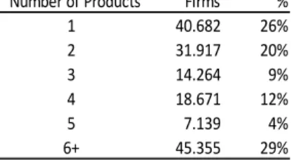
characterized by few sellers, with the power to set prices above marginal costs and many price-taking buyers. If the firm was inserted in a perfectly competitive market, the mark-up would be equal to one, since the price would be equal to the marginal cost. The standard approach in the literature is to use a sectorial classification as a market segmentation. The assumption is that firms sell one good and compete in only one market. Therefore, multi-product firms are a source of bias, especially if products are not close substitutes. Apart from that, my option for single-product firms concerns the difficulty of identifying concretely and specifically the inputs allocation, i.e. the portion applied of each input used in different production processes. Besides this assumption, there is a difficulty in specifying multi-product production functions, since there is huge diversity in the nature of outputs estimated and since there are multiple equations that are needed and a large number of restrictions for each one. As we can see in table IX in appendix A.1, around 26 per cent of the sample are single-product firms and, from these, I selected industries that had a sufficient number of firms each year to allow for estimation, i.e. more or less 20 per year on average. This option may raise some criticism since the inclusion of multi-product firms would guarantee a higher representativeness, because most firms produce more than one product.
Finally, the option for the median mark-up, instead of the average mark-up, which is more common in the literature, addresses the fact that the average may not be a robust tool, since it is largely influenced by outliers. Apart from that, the median is better suited for skewed distributions to derive to a central tendency.
The mark-up level, that here is the price-marginal cost ratio, is defined as
(1) !!"#=
!!"# !"!"# ,
where !!"# represents the price of good j for firm i at time t. I assume that firm i
10
(2) !!"#= !! !!"#, !!"#, !!"#, !!"# ,
where !!"#!represents the quantity of good j produced by firm i at time t, !!"#!stands for
the physical capital stock held by the firm, !!"# is labour, !!"# stands for materials
(intermediate inputs), and !!"# stands for unobservable total factor productivity (TFP). If the firm maximizes its profits, its marginal cost is given by
(3) !"!"#=
!!"#! !"#!"#!,
where ! = K, L, M and !"#!"#, is the marginal product of input !, and p!"#! represents
its price, with !!"#! = !
!" being the nominal wage rate, !!"#! = !!",! is the rental price of
capital and!!!!"#! is the price of the materials.
Considering the marginal product of ! is given by (4) !"#!"# =
!"!
!"!"# !!"#, !!"#, !!"#, !!"# !,
Thus, if we substitute eq. (3) and (4) in (1), we obtain !!"!= !!"# !!"! !"!!"#= !!"#! !"#!"# !"#!"#!, where !!"#! =!!"!!!"#
!!"# is cost share of input ! as a proportion of total revenue !!"#=
!!"#!!"# and !"#!"#= !!"#
!!"# is the average product of input !. In my model I will focus
on intermediate inputs (materials). This option addresses the fact that it is less costly to adjust the usage of materials than that of labour. In the literature presented in section 2, labour is the most common input factor used.
Let !!"#! =!"#!"#
!"#!"# denote the input elasticity and so that eq. (1) can be written as
(5) !!"#! =!!"#
!
!!"# Thus, we obtain a system with two equations:
11
(6) !" !!"#= ! !" !! !!"#, !!"#, !!"#, !!"# !" !!"# = !" !!! !
!"#, !!"#, !!"#, !!"# −!!" !!"#!
In this system, we need only to estimate the first equation. From the estimation procedure we identify !!!!,!the input’s elasticity, and !
!"#! , the cost share of the input, is
obtained from the data. In the system above, we have only two unobservable variables: !!"# and!!!"#.
Let us assume a Cobb-Douglas production specification for eq. (2): ! !!"# = !!"#!!"#!!!
!"# !!!
!"# !!
where !!, !!, !!!! 0,1 . In this case, we obtain !!"#! = !
!, !! or !!, i.e. the output
elasticity of the inputs is constant. Since I assumed a Cobb-Douglas6 production function, the technology is Hicks-neutral. Therefore eq. (6) becomes:
ln !!"#= !!ln !!"#+ !!ln !!"#+!!ln !!"#+ ln !!"# ln !!"#= ! ln !!− ln !!"#!
As Olley & Pakes (1996), Levinshon & Petrin (2003) and Ackerberg et al. (2006) pointed out, the input-endogeneity problem arises once TFP and mark-ups are unobserved and correlated with inputs. Following Olley & Pakes (1996), I introduce a standard Markovian assumption about the TFP stochastic process.
Assumption 1: Productivity evolves according to a first-order Markov process given by
(7) ln !!"# = ! ln !!,!!! + !!"!,
where g(.) is a general function and !!" is i.i.d. over i and over t .
Since I assume that TFP follows a first-order Markov process in a model that has a dynamic common factor representation, there is no need to specify input demand
6 The option for a Cobb-Douglas production function concerns the fact that it is easier and simpler to
estimate and to interpret and requires estimation of a small number of parameters when compared to a Translog. Besides this fact, it has one main advantage, which is that all firms have the same production elasticities and that substitution elasticities equal one. For other examples of production functions, like Translog, see, for example, Santos et al. (2014) or Gandhi et al. (2013).
12
functions – see further information in Blundell and Bond (2000)7. Under this assumption, state variables are uncorrelated. Violations of the Markov assumption will generate serial correlation and !!" would be correlated with the state variables, and this instrument would not be valid8. Furthermore, predetermined variables are also valid instruments, e.g. the capital stock or labour (especially skilled labour) when it is chosen at the end of period t-1.
Therefore, if we substitute eq. (7) in the Cobb-Douglas case, our estimating equation becomes:
(8)
ln !!"#= ! !!ln !!"#+ !!ln !!"#+!!ln !!"#+ ln !!"# = !!ln !!"#+ !!ln !!"#+!!ln !!"#+
! ln !!",!!!− !!ln !!",!!!− !!ln !!",!!!−!!ln !!",!!! + !!"
Following Hu & Shum (2012) once more, the generalized method of moments (GMM) estimator uses the following orthogonality conditions:
(9) ! !!" ℎ! ! !",!!!, !!",!!!, !!",!!!, !!",!!!! … ℎ! ! !",!!!, !!",!!!, !!",!!!, !!",!!!! !!" !!" = 0
where ℎ!(.) for p = 1,…, P are polynomials of order p. The GMM estimator is used
eliminate unobserved firm-specific effects.
7 The common factor is !
!", since it connects different coefficients on the same variable with a first or
higer-order difference lag.
13
4 D
ATA DESCRIPTIONThe dataset consists of an annual frequency panel ranging from 2004 to 2010, including price data. This allows me to avoid the problem identified by Klette & Griliches (1996) when using revenues instead of quantities.
The dataset was constructed from two sources. The first data source is a sample of firms surveyed: IAPI (Inquérito Anual à Produção Industrial), available for the period of 1992-2011 and containing very detailed 12-digit product information, including total revenues and quantities, both produced and sold. Prices are collected for each firm and each product. This survey covers roughly 8,000 firms per year and an average of nearly 42,000 products per year. The second source is a census of firm-level financial data: IES (Informação Empresarial Simplificada), available for the period of 2004-2010 and covering all domestic firms. For my analysis, I considerer manufacturing industries that do not belong to sole proprietors. This source covers around 1 million firms per year, but after these exclusions, the universe of registered firms is around 300,000 per year. This census has financial information, usually presented in balance sheets and some employment and investment statistics.
IES had a previous version, though it was a survey instead of a census, named IEH (Inquérito às Empresas Harmonizado), available for the period of 1996-2004. However, since it covered a sample of the firm population, it did not contain full information and it was difficult to cross it with IAPI, because the samples were independently drawn. Besides this, I also restrict myself to industries with, at least, 20 observations per year, on average, in order not to obtain biased estimations due to small sample sizes.
Another important issue is the selection criteria of single-product firms and the level of aggregation. As the information on products is very detailed, I aggregate it at 5 and 7 digits, instead of at a 12-digit product level, taking into account the measurement
14
units. The measurement units criterion also excludes some industries, since it is not plausible to match different measurement units (e.g. litres with pounds), and, therefore, this would lead to biased estimations.
The selection criterion of single-product firms also consists in setting a minimum proportion of revenues originated by the firm’s most important product.
Another important issue is the definition of variables. The set of variables required to estimate eq. (7) is relatively wide. Firstly, I exclude all firms that have less than 3 employees. This option adresses the low variability of employment in this kind of firms.
The physical capital stock is always quite difficult to measure. The measurement of physical capital stock presented here follows the perpetual-inventory method (PIM)9. Applying the measures of assets and investment presented in the data I use the following equation:
(10) !!!!= !! 1 − ! + (!!"#!− !"#$%&!) ,
where !!" is the investment and !"#$!" is the desinvestment. The depreciation rate of manufacturing industries10 (!),!was constructed using the variables taken from the European Commission AMECO database.
Finally, the intermediate inputs were measured by adding the series of cost of goods sold and consumed and supplies and services. In eq. (11), I present a price deflator for intermediate inputs that is common to all the firms:
(11) !! = !! !! !!−!"!!! !! = 1!!"#!! = 2004 !! = 1!!"#!! = 2004 9
PIM is a method of constructing estimates for the physical capital stock and consumption of fixed capital from time series of gross fixed capital formation.
15
where !! is the price deflator of intermediate inputs; !!!stands for the intermediate
inputs, constructed through IES; !" represents revenues; !!!represents the price index for output; !"! stands for nominal value added and !! is the price index for value added.11 The following equations represent the price index of output and value added, respectively: !!,! = !!!,!!! !!,! !!,!!! and !!,! = ! !!,!!! !"!,! !"!,!!! .
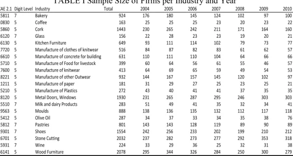
Concerning all these assumptions, I adduce table I, which presents the sample size of firms per industry and year of single-product firms with 100 per cent of total revenues as the selection criterion. This selection criterion leads me to a sample that represents just 5 per cent of usable sample firms, i.e more or less 350.00, as we can see in table XI appendix A.1, and that fact, may not guarantee the representativeness required.12 This classification and choice of single-product firms can be criticised as being too simplistic, although it is a good starting point for analysing the levels of mark-ups.
11 The variables were taken from Instituto Nacional de Estatística (INE): !"
! – C.1.2.1 ; !"#! –
A.1.4.4.1
12 See for instance, in appendix A.1 a set of tables with the information of the dataset selection and a
16
TABLE I Sample Size of Firms per Industry and Year
5 E
MPIRICALA
NALYSIS5.1 Interpretation and Possible Estimation Biases
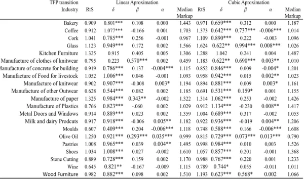
The results of the estimation of the production function in eq. (8), using both linear and cubic polynomials to approach the stochastic process for productivity, and using the share of intermediate inputs to measure mark-ups, are presented in Table II13. Besides the estimation of the production function with GMM, I also tried using Ordinary Least Squares (OLS). The results are presented in Appendix B.1 and, as expected and pointed out in the literature, OLS estimations of the coefficients are biased and inconsistent14.
13 Estimates for the coefficients and standard errors and values of the g(.) function in eq. (8) are presented
in Table XVIII as are estimations for the same equation but with just capital stock as an instrument, i.e. when labour and intermediate inputs are not predetermined.
14What is shown in Appendix B.1 are the results of the OLS estimation of a Cobb-Douglas production function for quantities, revenues, and value added. Two cases are presented. The first one does not consider intermediate inputs and the mark-up is measured by labour share. The second one may include intermediate inputs and the mark-up is obtained from the materials share. In Appendix B.3, we can find estimations for the following topics: i) GMM estimations using labour share to measure mark-up in Table XX, ii) GMM estimations using both labour and intermediate inputs share to measure mark-up in Table XXII, iii) GMM estimations using labour share to measure mark-up, without intermediate inputs in Table XXI.
CAE$2.1 Digit$Level Industry$ Total 2004 2005 2006 2007 2008 2009 2010
15811 7 Bakery 924 176 180 145 124 102 97 100 10830 5 Coffee 163 25 25 25 23 20 23 22 15860 5 Cork 1443 230 265 242 211 171 164 160 26120 7 Glass 156 22 28 23 23 19 20 21 36130 5 Kitchen$Furniture 649 93 111 114 102 79 73 77 17720 5 Manufacture$of$clothes$of$knitwear 516 84 87 82 83 61 62 57 26610 5 Manufacture$of$concrete$for$building 631 110 111 110 104 64 66 66 15710 5 Manufacture$of$Food$for$livestock 399 60 64 56 61 55 46 57 17600 5 Manufacture$of$knitwear 413 64 69 65 59 49 54 53 18221 5 Manufacture$of$other$Outwear 932 144 167 157 145 120 102 97 21211 5 Manufacture$of$paper 181 31 29 27 25 23 25 21 25210 5 Manufacture$of$Plastics 272 43 40 41 41 37 35 35 28120 5 Metal$Doors,$Windows 1930 231 265 287 295 246 303 303 15510 7 Milk$and$dairy$Products 283 51 49 41 35 32 34 41 29563 5 Moulds 888 138 136 135 132 112 117 118 15412 5 Olive$Oil 287 34 37 33 34 35 38 76 15812 7 Pastries 801 143 143 128 119 89 90 89 19301 7 Shoes 1554 242 256 233 202 199 210 212 26701 5 Stone$Cutting 2032 237 282 273 277 292 353 318 15931 7 Wine 224 33 29 36 25 32 31 38 36141 5 Wood$Furniture 2078 295 344 326 284 250 300 279 Source:$Author's$Computation Note:$Number$of$firms$per$year$at$100%$criteria$at$5$and$7$digits$level$aggregation$of$product$code$between$2004X2010
17
Figures 6 to 11, shown in Appendix B.1, exhibit a comparison of mark-ups estimated with quantities, revenues and value added as dependent variables using OLS15.
TABLE II GMM Estimates for the Coefficients of the Production Function TFP transition Industry RtS δ β α Median Markup RtS δ β α Median Markup Bakery 0.909 0.801*** 0.108 0.000 1.443 0.971 0.659*** 0.312 0.000 1.187 Coffee 0.912 1.077*** -0.166 0.001 1.703 1.373 0.642*** 0.737*** -0.006*** 1.014 Cork 1.041 0.785*** 0.256 -0.001 0.967 1.109 0.890*** 0.222 -0.003 1.096 Glass 1.123 0.949*** 0.172 0.002 1.566 1.624 0.622** 0.994*** 0.008*** 1.026 Kitchen Furniture 1.325 0.915 0.405 0.005 1.306 1.288 1.042 0.241 0.004 1.487 Manufacture of clothes of knitwear 0.795 0.223 0.570*** 0.002 0.459 1.183 0.622** 0.690*** 0.003** 1.010 Manufacture of concrete for building 0.919 0.786*** 0.137 -0.004*** 1.115 0.852 0.846*** 0.009 -0.004* 1.201 Manufacture of Food for livestock 1.052 1.006*** 0.046 -0.001 1.093 0.958 0.942*** 0.015 0.002** 1.023 Manufacture of knitwear 0.902 0.907*** -0.008 0.003* 1.194 0.894 0.881*** 0.009 0.003* 1.161 Manufacture of other Outwear 0.628 0.544*** 0.082 0.002 1.185 0.691 0.531*** 0.159* 0.001 1.155 Manufacture of paper 1.325 0.984*** 0.343** -0.002 1.322 1.314 1.062*** 0.253 -0.002 1.426 Manufacture of Plastics 0.766 0.823*** -.060 0.002 1.029 0.912 1.134*** -0.230 0.008** 1.417 Metal Doors and Windows 0.914 0.889*** 0.023 0.002 1.359 1.004 0.689*** 0.317 -0.002 1.053 Milk and dairy Prodcuts 0.917 0.918*** -0.006 0.005** 1.182 0.922 0.936*** -0.019 0.004** 1.206 Moulds 0.607 0.409*** 0.204 -0.006*** 1.118 0.748 0.588*** 0.166 -0.006*** 1.608 Olive Oil 1.250 0.921*** 0.293*** 0.035*** 0.999 0.815 0.729*** 0.073*** 0.013*** 0.790 Pastries 1.008 0.965*** 0.039 0.004** 1.495 0.998 0.984*** 0.010 0,003 1.526 Shoes 1.034 1.008*** 0.027 -0.002 1.610 1.057 0.857*** 0.201 -0.001 1.368 Stone Cutting 0.889 0.728*** 0.159 0.002 1.170 0.988 0.767*** 0.220 0.001 1.233 Wine 0.645 0.821** -0.167 -0.009 1.115 0.789 0.744* 0.055 -0.011 1.011 Wood$Furniture 0.982 0.882*** 0.098 0.002 1.510 1.193 0.623*** 0.568* 0.002 1.066
Linear Aproximation Cubic Aproximation
Source:$Author's$Computation
Nothes:$The$set$of$instruments$is$the$level$of$capital$stock$and$employment$together$with$linear$terms$(for$linear$approximation),$ quadratic$and$cubic$terms$(for$cubic$approximation)$of$all$variables$lagged$one$period.
*,**,***$denotes$statistacally$significant$at$10,$5$and$1$per$cent$level,$respectively.
First, the column presenting the levels of returns to scale (RtS), in Table II, shows us that most industries exhibit constant returns to scale, i.e. the values for !!+ !!+ !! that are close to one. However, Moulds and Wine may show decreasing RtS. On the other hand, Manufacture of paper, and Metal doors and Windows may exhibit increasing RtS. Table III presents the results of the formal t-test described above. The following statistical test has a greater importance because some industries exhibit a small sample size and this may lead to spurious coefficients. We can observe, in Table III, that, at 1 per cent significance, only Olive oil and Manufacture of outwear reject the hypothesis
15 From these results, we can conclude that quantities produce higher mark-ups when compared to
revenues, but lower when compared to value added, using the labour share to measure mark-ups. If we introduce intermediate inputs, the mark-ups are higher when quantities are used as a dependent variable, instead of revenues or value added.
18
of constant returns to scale for both approximations. These results are similar to the ones presented in the previous paragraph.
TABLE III Returns to Scale Test at 1 per cent significance Linear Cubic Industry p-stat p-stat Bakery 0.258 0.791 Coffee 0.395 0.000 Cork 0.760 0.529 Glass 0.571 0.000 Kitchen Furniture 0.137 0.421 Manufacture of Clothes of Knitwear 0.128 0.298 Manufacture of Concrete for Building 0.545 0.366 Manufacture of Food for Livestock 0.506 0.155 Manufacture of Knitwear 0.282 0.065 Manufacture of other Outwear 0.000 0.000 Manufacture of Paper 0.038 0.007 Manufacture of Plastics 0.000 0.527 Metal Doors and Windows 0.203 0.957 Milk and Dairy Products 0.162 0.238 Moulds 0.026 0.157 Olive Oil 0.002 0.000 Pastries 0.898 0.976 Shoes 0.625 0.477 Stone Cutting 0.271 0.957 Wine 0.171 0.802 Wood Furniture 0.784 0.210 Source: Author's computation
P-Stat represents the probability of RtS being different from one
Another important issue are the values estimated for the coefficients. The low values obtained for !, in some cases even negative, e.g. Coffee or Moulds, are odd from an economic point of view. The low or non-significant estimates may be due to the fact that the time dimension of the panel is short and the physical capital stock does not have enough time variability at the firm level.
On the other hand, we can observe high values for the estimates of !, the elasticity of materials, as I assume that the input factors are substitutes and that intermediate inputs are easily adjusted by the firm, allowing for higher variability.
The estimated values for ! are usually positive, with some exceptions, e.g. Manufacture of knitwear, Manufacture of plastics, Milk and dairy products and Wine. As we can see in Table II, none of them is statistically significant. It is important to
19
point out that most of the literature, e.g. Rotemberg & Woodford (1999), amongst others, do not use intermediate inputs or materials, but labour to estimate the mark-up.
Also, it is important to explore the validity of the instruments used. The analysis of the validity is presented in Table IV, which contains the results for the Sargan-Hansen statistical test. The joint null hypothesis is that the instruments used are valid, i.e. that they are uncorrelated with residuals. We can observe that, at 5 per cent significance, only in Manufacture of outwear and in Manufacture of concrete for building is the null hypothesis rejected, i.e. the instruments may not be valid for this equation or they may be incorrectly used. Considering the cubic approximation instead of the linear one, results may differ, but not significantly. For the industries identified above, along with Olive oil and Wine, we reject the null hypothesis at 5 per cent significance.
TABLE IV Validity of the Instruments
Industry J Stat Degrees of Freedom P-Value J Stat Degrees of Freedom P-Value Bakery 10.002 12 0.616 9.817 7 0.196
Coffee 7.011 12 0.857 3.289 7 0.856
Cork 5.415 12 0.943 3.312 7 0.855 Glass 8.704 12 0.728 5.798 7 0.564 Kitchen Furniture 4.177 12 0.980 4.114 7 0.766
Manufacture of clothes of knitwear 17.146 12 0.144 9.009 7 0.252 Manufacture of concrete for building 22.836 12 0.029 20.992 7 0.04
Manufacture of Food for livestock 15.638 12 0.208 8.148 7 0.319
Manufacture of knitwear 6.064 12 0.913 2.895 7 0.895 Manufacture of other outwear 25.314 12 0.013 26.985 7 0.03
Manufacture of paper 12.984 12 0.370 7.361 7 0.392
Manufacture of Plastics 15.416 12 0.219 8.026 7 0.330
Metal Doors and Windows19.136 12 0.085 17.129 7 0.017 Milk and dairy Products 7.516 12 0.822 3.557 7 0.829
Moulds 12.370 12 0.416 9.978 7 0.254 Olive Oil12.606 12 0.398 12.863 7 0.095 Pastries 12.865 12 0.379 4.955 7 0.665 Shoes 7.027 12 0.856 4.123 7 0.766 Stone Cutting 20.871 12 0.052 17.445 7 0.126 Wine 5.854 12 0.923 5.078 7 0.065 Wood Furniture 18.101 12 0.113 2.111 7 0.953
Linear Approximation Cubic Approximation
Source:(Author's(computation(
Notes:(the(J5Stat(presented(is(The(Sargan5Hansen(test(
Another issue that is important to analyse are the values of the g(.) function presented in eq. (8). In Table II, we can observe a difference between the results of median mark-up for Coffee and Glass with linear and cubic approximations. Besides the
20
reasons previously mentioned, the values of the coefficients in the g(.) function also influence the results, as we can see in Table XIX, presented in appendix B.2. For the industries mentioned, it is possible to see the difference between the values of the g(.) function for the linear and cubic approaches, which consequently leads to a difference in estimated mark-ups. Also, and according to Klette & Griliches (1996), using quantities instead of revenues to estimate the production function results in higher mark-ups. The reason for this difference is related to the use of deflated sales as the dependent variable. The main idea is related to a cost improvement, when compared to the other firms of the industry, which allows for a reduction in the price and, therefore, expands the market share of the firm. It follows, due to the correction of relative prices, that replacing changes in real output by growth in deflated sales will introduce a bias in parameters. I did not address these kinds of problems, since my method uses the prices obtained by dividing revenues by quantities. This method provides more accurate estimates of the median mark-up level and allows us to understand its true value, i.e. the monopoly degree.
5.2 Interpreting Mark-ups
The industrial organization literature16 typically associates the mark-up level to a range of structural variables such as establishment size, capital intensity, vertical integration, economies of scale or scope, product differentiation, capital intensity, exposure to international competition, R&D, amongst others, although the rationale for mark-up levels differs depending on the type of industry. To identify the type of competition and relate it to the mark-up estimates, I will focus on a few indicators.
21 0! 0,2! 0,4! 0,6! 0,8! 1! 1,2! 1,4! 1,6! 1,8! 12! 12,5! 13! 13,5! 14! 14,5! 15! 15,5! 16! 16,5! Me di an 'Ma rk* up ' log'of'output'
The first indicator that I will analyse is the average firm size. The firm size is a proxy for the existence of size advantage, like scale economies at the firm level as pointed by Martins et al (1996). It is expected, in this kind of industries, that a large average firm size may exhibit large firms that cover a large percentage of the employment and of the output of the industry. For this reason, I analyse the relation between the median mark-up and the median size of each industry, taking into account the output, i.e. the volume of sales. As far as we can see in figure 1, in general, firms that exhibit a larger median output may tend to display smaller median mark-ups. This might be odd from an economic point of view, that firms do not take advantage of their respective size.
Figure 1- Median mark-up and log of median output by industry
It seems that mark-ups tend to be smaller in industries with a large average firm size, and these industries may indeed be closer to a state of perfect competition, although the heterogeneity of each industry might need a pattern more complex than the one presented in the figures. Besides this, it can be taken as a sign that a high degree of intra-industry competition or a high degree of product differentiation exist, which may lead to a difference in costs and prices, and, therefore, the mark-up level is close to one, i.e. does not allow the exercise of market power by the large firms of the industry. This
22
may be the example of the pastries industry once we are talking about different types of fresh pastry. The same can happen with glass industry, although, if we analyse the correlation between the median mark-up and the establishment size, it appears that the firm size does not have a significant correlation with the mark-up, as we can see in table XXIII in appendix B.4.
The second indicator is the capital intensity. From the capital intensity, some advantages may arise, such as: a) the scale economies, b) an increase in productivity., amongst others. Here, the capital intensity is analysed considering the ratio of the physical stock of capital, measured in thousands of euros, and the number of employees. Half of the 22 industries selected present a capital intensity ratio greater than 50 per cent, and it is curious to see that the industries that present a higher capital intensity are the ones that present, in general, smaller median mark-ups, with the exception of the production of Coffee, as can be seen in table XXIV, shown in appendix B.4. It is important to highlight, for example, the production of Cork, which, exhibits a large capital intensity ratio, shows a median mark-up level closer to one, i.e. there may not exist an advantage in the industry for being intensive in capital. As it happens with establishment size, this indicator appears to have no significant correlation with the mark-up level, as we can see in table XXIV.
These results are in line with such literature as Martins et. al. (1996), which analysis these two indicators and concludes that both appear to have no significant link with the mark-up.
Another important indicator may be the research and development at firm level, allowing to study the investment that each firm makes concerning the innovation and differentiation; however, the data do not make available the importance of R&D in the cost structure of the firm. In the same situation there are the entry barriers or the
23
exposure to international competition. Besides the fact that data do not have the export/import ratio, I will make a guess based on the knowledge surrounding the subject. Many firms that compete in international markets hope to gain cost advantages, mainly due to the attainment of economies of scale that lower their production costs. Nevertheless, this kind of industries, that are exposed to international competition, are also exposed to a new set of costumers, but, at the same time, to a higher level of competition and, therefore, mark-ups may be closer to one. Also, the product differentiation influences the results. Besides the fact that external or internal competition may reduce the market power, if we are comparing very different products, the costs and the prices may necessarily be different, e.g. the Wine industry or textile sector.
5.3 Comparison with previous studies
The results were expected since mark-up expresses the power that a firm has to set a price above its marginal cost. Nevertheless, some industries may exhibit a median mark-up lower than 1, e.g. Olive oil, Cork and Manufacture of knitwear clothing, which was not expected and can be odd from an economic point of view, i.e. a firm sells at a price below the cost of the last unit; however, I did not impose any restrictions in order for mark-ups to be larger than one. The results of mark-ups obtained for manufacturing industries range, with some exceptions, from zero to 50 per cent and are, in general, above 15 per cent. These values are substantially lower than the ones reported by Santos
et. al. (2014), which are, in general, above 20 per cent for the Portuguese manufacturing
sector. In broad terms, the difference between these results is primarily due to the adjustment of intermediate inputs. In the results reported by Hall (1988), the significant mark-up ratios are clearly above 100 per cent, which is similar to Roeger’s (1995) results for the U.S. manufacturing sector, that range from 15 to 175 per cent. The results
24
presented in this paper are more in line with those of Martins et. al. (1996), where the mark-up level ranges between zero to 30 per cent.
5.4 Mark-up and TFP distributions
Besides all these hypothesis, it is important to analyse the distribution of mark-up and TFP distributions, taking into consideration some of the problems presented above.
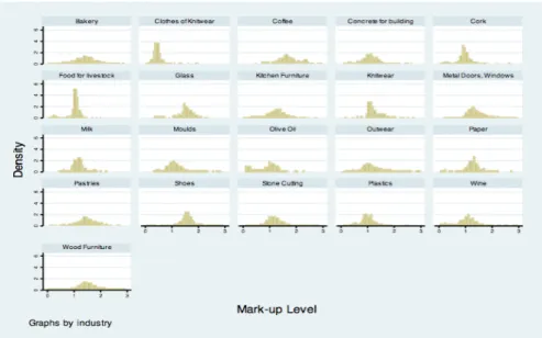
Table II shows a median mark-up level in each industry. However, there is a large amount of heterogeneity that empirically arises from the shares of inputs to the production function approach, even when we consider similar technologies. Figure 2 depicts the distribution of firm’s ups in each industry. The distributions of mark-ups in some of the industries look like a Gaussian distribution17, e.g. Bakery, Coffee, Kitchen furniture, Metal doors and windows, Milk and dairy products, Moulds, Manufacture of other outwear, Pastries, and Wood furniture. The other industries tend to be more asymmetric, e.g. Manufacture of food for livestock.
From the Kolmogrov-Smirnov non-parametric test, I conclude that, at 5 per cent of significance, results may differ in the shape of distributions presented in Figure 2. This type of behavior is expected since we did not impose any mark-up restrictions to be larger than one, and there are always some measurement errors that are present when the mark-up is smaller than one, as shown in the figure.
Notice that the coefficient of intermediate inputs influences only the median mark-up level. So, even if we had assumed similar technologies across industries, the intermediate input share would still change from one firm or industry to another, i.e. there is a large amount of heterogeneity across industries. However, industries that present more homogeneous products, such as Cork, tend to show less dispersion than
25
Bakery or Manufacture of other outwear. Moulds, for instance, present a mark-up distribution that is closer to a state of perfect competition and a long tail of producers with high market power, in an industry where there is not much product differentiation, this being the reason why it is measured by the number of moulds produced. Other examples are the production of olive oil or the manufacture of concrete for building.
Figure 2- Mark-up Distribution by Firm for Each Industry
26
Figure 3 shows us the firm distribution TFP for each industry. The logarithm of TFP seems to have a Gaussian distribution, which implies a lognormal distribution for TFP levels. As we can observe, there is a significant dispersion of firm TFP across the same industry, e.g. Kitchen furniture. This may happen due to products’ heterogeneity within industry, e.g. in the Kitchen furniture industry, the unit considered is the number of pieces used to construct each part of the furniture, meaning one cupboard or one table.
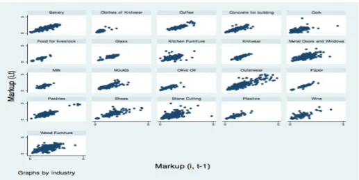
Figures 4 and 5 depict the persistency in mark-up and TFP levels obtained for each firm, i.e. in materials shares across firms in the same industry. Market power measures tend to exhibit a high persistency18, but not as high as TFP. To analyse the persistency, I present, in Table XXVI, appendix B.5, a formal ADF unit-root test. The null hypothesis tests the correlation between the variable at time t and t-1. As we can see from the results, we cannot reject the existence of a unit root, i.e. there is a correlation of mark-ups between period t and t-1. The same occurs when we consider the TFP. We can observe this in Bakery and Wood furniture, shown in figure 5. The smaller dispersion might be a sign of the fact that the industry may have a more dynamic market structure in more homogeneous industries. This may be an indication that firms compete more with each other in more homogeneous industries and for more homogeneous products. This may also be a sign of the fact that industries which show less dispersion tend to be more competitive. See, for example, Olive oil, which presents a mark-up close to one, in an industry with small product differentiation, since we are talking about the production of litres of olive oil.
27
Figure 4- Mark-up Transition by Industry
Figure 5- TFP Transition by Industry
6 C
YCLICALITY WITHGDP
The cyclicality of mark-ups is one of the topics that raise most interest in macroeconomic literature nowadays19. In this section, as a first approximation to the analysis of cyclicality of mark-ups, I analyse it in relation to the logarithm of GDP, which will be followed by a brief study of unconditional cyclicality of mark-ups with prices, quantities, revenues and value added.
19 See Afonso & Costa (2013), Nekarda & Ramey (2013) and Juessen & Linnemann (2012), amongst
28
Nekarda & Ramey (2013), Rotemberg & Woodford (1999), amongst others, analyse the behavior of mark-ups concerning the GDP, as well as the effect of shocks of supply and demand. Therefore, I assess the cyclicality by computing the correlation of mark-ups with the GDP with fixed effects. The GDP at constant prices was taken from the European Commission AMECO database (1.1.0.0.OVGD).
Table V shows the results of the following equation: (12) !!"= ! !!!" !"#!+ !! +!!!"
where !! represents firm’s dummies.
TABLE V Mark-up Regression with GDP: Estimated Values in eq. (12) Coef. s. e. Coef. s. e. ln(GDP) -0.484*** 0.13 -0.10*** 0.03 Constant 3.89*** 0.59 2.19*** 0.12 R-Squared 0.002 0.04 Prob>F 0.000 0.000 Observations 16285 1438911 Firms 4299 364528
Source: Author's computation
Notes: The sample results are for the selected industries. In the whole economy the dependent variable is the inverse of the input share for materials and the whole census data is used. *** significant at 1 per cent
Sample Whole economy
As we can see in Table V, the market power measure tends to have a negative correlation with the GDP log. This is also true for the whole economy, which represents the whole set of firms presented in the IES. Our results are similar to the ones that are presented in the literature, e.g. Santos et al. (2014). Considering other assesses of the unconditional cyclicality, I compute the correlation of mark-ups with prices, quantities, revenues and value added.
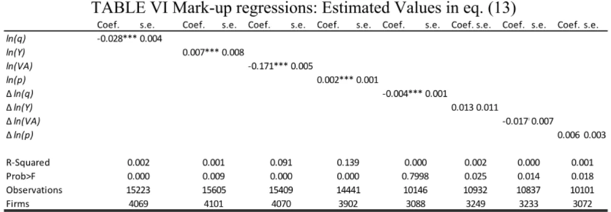
The results shown in Table VI, are obtained through the following equation: (13) !" !!"= !!!" !!"+!!!+!!!"
29
TABLE VI Mark-up regressions: Estimated Values in eq. (13)
Concerning the results in Table VI, we can see that the mark-up is positively correlated to prices and negatively to quantities. This was expected since demand functions are downward slopping. The results of both tables are as expected. Rotemberg & Woodford (1999), for example, use the evidence on the pro-cyclical behavior of input factors to conclude that average mark-ups are unconditionally countercyclical, although the pro-cyclical behavior of inputs itself does not guarantee the counter-cyclicality of mark-ups with GDP. A deeper analysis is necessary concerning the supply and demand shocks, even more when the mark-up depends not on input utilization but on the share of one input, in this case an intermediate input. Nonetheless, this is a preliminary indication of the fact that mark-ups tend to be countercyclical with shocks that affect the GDP. Also, as explained by many authors, namely Rotemberg & Woodford (1999), mark-up variations contribute to output movements, even if these are independent from the real marginal cost shift and even if there is a negative correlation between them. This relation between output and mark-ups plays an important role, mostly due to effects concerning shocks, as for example the technology shocks. If those shocks induce countercyclical markup variations, this will further amplify their effects upon the output, in addition to the effects that come from marginal cost variations. The argument for value-added and revenues is the same as for output, and the correlation between
Coef. s.e. Coef. s.e. Coef. s.e. Coef. s.e. Coef. s.e. Coef. s.e. Coef. s.e. Coef. s.e.
ln(q) '0.028*** 0.004 ln(Y) 0.007*** 0.008 ln(VA) '0.171*** 0.005 ln(p) 0.002*** 0.001 Δ"ln(q) '0.004*** 0.001 Δ*ln(Y) 0.013 0.011 Δ"ln(VA) '0.017**0.007 Δ"ln(p) 0.006 0.003 R'Squared Prob>F Observations Firms 10146 10932 10837 10101 Source:FAuthor'sFComputationF Notes:F***,**,*FdenotesFstatiscallyFsignificantFatF1,5FandF10FperFcentFlevel,Frespectively qFrepresentsFquantities,FYFstandsFforFrevenues,FVAFstandsFforFValue'Added;FpFrepresentsFprices 3088 3249 3233 3072 4069 4101 4070 3902 0.002 0.000 0.001 0.7998 0.025 0.014 0.018 0.002 0.001 0.091 0.139 0.000 0.000 15223 0.000 14441 0.009 15605 0.000 15409
30
them and mark-ups is also negative. Hall (2009) for instance, presents a point of view stating that models where mark-up falls when output expands are due to sticky prices of products.
From a policy point of view, the cyclicality of mark-ups is largely influenced by the effectiveness of the economics policy. For these reasons, some shocks are identified by the literature mainly due to productivity, taxation, government spending, amongst others. Nowadays, there is a renewed interest in the effects of fiscal policy, which resulted in a series of papers (e.g. Afonso & Costa (2013)); this is also true for government-spending (e.g. Hall(2009))
New Keynesisan synthesis models produced undesired endogenous mark-ups due to nominal rigidity, highlighting the effectiveness of demand-side policy when compared to real business cycle models, as explained by Afonso & Costa (2013) or Rotemberg & Woodford (1999). Goodfriend & King (1997), analyse the neoclassical synthesis and the role of monetary policy and conclude that mark-ups are counter-cyclical mainly due to nominal rigidity and to the costly dynamic of prices adjustment. Therefore, it occurs that mark-up reduction arises with an increase in ouput. Concerning government spending, Hall (2009) presents a point-of-view stating that there is an increase in total output when the government buys more goods and services.
When we consider the case of desired mark-ups, see for example Ravn et al. (2006), that relates productivity shocks in the presence of fiscal shocks.
To sum up, the theoretical literature on mark-ups is largely dominated by the idea that mark-ups behave pro-cyclically with supply shocks and counter-cyclically with demand shocks.
31
7 C
ONCLUSIONThis dissertation aims to provide new insights on the estimation of mark-up levels in Portuguese manufacturing industries by using a plant rich price and quantity data, where information on prices allows estimating production function in quantities instead of revenues. The first conclusion is that the former approach produces higher mark-ups than the latter.
I used a GMM approach that combines quantities, labour, physical stock of capital, or intermediate inputs, and lags of the variables as instruments. Due to the fact the optimal choice of inputs may lead to an input-endogeneity problem, I presented a new way of estimating the production function under mild assumptions for the productivity stochastic process, based upon the recent work of Santos et al. (2014).
The analysis for 21 manufacturing industries using single-product firms in the period of 2004-2010 shows that, price-marginal cost ratios are substantially larger than one in general, usually above 15 per cent.
I have also conducted an empirical analysis of mark-up (and TFP) distributions for each industry and I provide some explanations about the mark-up level. The main conclusion in this front is that there is a large amount of heterogeneity amongst firms and industries. Furthermore, industries that show less dispersion, tend to more competitive.
Finally, I study the unconditional cyclicality of mark-up with respect to GDP, prices, quantities, revenues and value added. I conclude that mark-ups tend to be countercyclical with GDP, quantities, revenues and value added, and procyclical with prices.
Considering the mark-ups are generally accepted to be procyclical with supply (i.e. TFP) shocks, the evidence here tends to favour the vision that mark-ups may be
32
countercyclical with demand shocks. However, I cannot advance that conclusion since I did not identify demand shocks separately in order to perform a condition cyclicality analysis.
In terms o future research, this dissertation opens the door to continue a detailed study on mark-ups in Portugal, with different production functions, less restrictive assumptions, and also for multi-product firms, especially using a cost-function approach.
33
R
EFERENCESAckerberg, D. K., Caves, K. & Frazer, G. (2006). Structural Identification of Production Functions. MPRA Papers, 38349
Afonso, A. & Costa, L. (2010) Market Power and Fiscal Policy in OECD Countries.
Applied Economics, 45, 4509-4555
Amador, J. & Soares, A.C. (2012) Competition in the Portuguese economy: an overview of classical indicators, Bank of Portugal Working Paper 8
Arellano, M. & Bond, S. (1991). Some Tests of Specification for Panel Data: Monte Carlo evidence and an application to employment equations. Review of Economic
Studies 58, 277–297
Blundell, R. & Bond. S. (2000). GMM Estimation with Persistent Panel Data: An application to production functions. Econometric Reviews- 71, 655-679
Blundell, R. and Powell, J. (2004) Endogeneity in semiparametric binary response models. Review of Economic Studies, 19, 321-340
Bond, S. & Soderbom, M. (2005). Adjustment Costs and the Identification of Cobb Douglas Production Functions. IFS Working Papers, WP05/04
Christopoulou R. & Vermeulen, P. (2012). Mark-ups in the Euro Area and the US over the Period 1981-2004: A comparison of 50 sectors. Empirical Economics, 42, 53-77
De Loecker, J. (2011). Product Differentiation, Multi-Product Firms and Estimating the Impact of Trade Liberalization on Productivity. Econometrica, 79, 1407-1451
34
Gandhi, A., Navarro, S. & Rivers, D. (2013). On the Identification of Production Funtions: How heterogeneous is productivity? 2012 Meeting Papers - Society of
Economics Dynamics, 105
Goodfriend, M. & King, R. (1997) The new neo-classical synthesis and the role of monetary policy, NBER Macroeconomics Annual 12, 231–83.
Hall, R. (1988). The Relation between Price and Marginal Cost in U.S. Industry. The
Journal of Political Economy 96, 921–947.
Hall, R. (2009). By how much does GDP rise if the government buys more output?,
Brookings Papers on Economic Activity 40, 183–249
Hu, Y. & Shum, M. (2012). Nonparametric Identification of Dynamic Models with Un- observed State Variables. Journal of Econometrics, 171, 32-44
INE (2014). Contas Nacionais – [Database], September 2014. Lisboa. Available at: http://www.ine.pt/xportal/xmain?xpid=INE&xpgid=ine_cnacionais
Klette, T. & Griliches, Z. (1996) The Inconsistency of Common Scale Estimators when Output Prices are Unobserved and Endogenous. Journal of Applied Econometrics, 11, 343-361
Juessen, F. & Linnemann, L. (2012) Markups and Fiscal Transmission in a Panel of OECD Countries. Journal of Macroeconomics, 34, 674-688
Levinsohn, J. & Petrin, A. (2003). Estimating Production Functions Using Inputs to Control for Unobservables. Review of Economic Studies, 70, 317-341