Is the low volatility anomaly still persistent? : it depends!

(1)

Is the Low Volatility Anomaly still persistent? It depends!

Maria Joana Farinha 152112062

Abstract

According to the methodology in Ang et al. (2009), we find that monthly stock excess returns are negatively related to the one-month lagged firm idiosyncratic volatility, across the U.S. with data spanning from June 1962 to December 2012. We show that the Low Volatility Anomaly disappears after controlling for price momentum for the overall market, which leads us to perform a deeper analysis. We segment the market by industry and find that, across 49 industries, the Food Products sector is the only one evidencing higher returns on low volatility stocks, even after controlling for market returns, size, value, long- and short-term momentum. An investment strategy that goes long on the low volatility portfolio and short on the high volatility portfolio within this sector is highly profitable, outperforming largely both the S&P500 and the DJIA indexes in 14% per annum, on average.

Professor José Faias Supervisor

Dissertation submitted in partial fulfillment of requirements for the degree of MSc in Business Administration, at Universidade Católica Portuguesa, March 2014.

(2)

Acknowledgements

My main motivation for engaging in this Empirical Finance thesis fully emerged from the great experience and knowledge acquired from the Methods in Finance course that I took on the last semester of my master’s degree.

Foremost, I would like to thank my supervisor Professor José Faias for his unconditional dedication, support, patience and problem-solving capability over all the obstacles faced during this dissertation. His expertise, goal-oriented and structured thoughts were undoubtedly key drivers for the quality achieved. In addition, I would also like to thank José Silva for teaching me the basic knowledge on MatLab programming, which was crucial for this thesis’ analytical development. Further, thanks to all my thesis colleagues for the great and stressful moments shared along this important stage of my life and to Fundação para a Ciência e Tecnologia for financial and data support.

I also sincerely thank my parents and Luisa for providing me the opportunity of studying in this amazing school and learning from the best, and mostly important, for the emotional support and care during my path.

On top of, a special thank you to Filipe not only for his guidance and helpful advice on work-related issues, but also for his continuous support and dedication throughout the countless failure moments, which I always overcame with him by my side.

(3)

Index of Tables

Table 1 - Summary Statistics ... 6

Table 2 - Cross-sectional Standard and Weighted Fama-MacBeth regressions ... 9

Table 3 - Recession vs Expansion periods ... 13

Table 4 - Descriptive Statistics and FF-3 alphas on IVOL portfolios ... 14

Table 5 - Long-Short portfolio time-series regressions ... 16

Table 6 - Descriptive Statistics across industries ... 19

Table 7 - Comparison of the Food Products industry with the remaining industries ... 24

Table 8 - 1-5 Food Products: Expansion vs Recession ... 25

Index of Figures

Figure 1 – Evolution of Total Volatility and Idiosyncratic Volatility ... 7

Figure 2 – Evolution of IVOL quintile portfolios ... 10

Figure 3 – Evolution of IVOL quintile portfolios in different starting times ... 11

Figure 4 – Comparison of the Low-High IVOL portfolio with the S&P500, DJIA and CRSP indexes ... 11

Figure 5 – Evolution of long low IVOL, short high IVOL and S&P500 ... 12

Figure 6 – 10-Industry High-Low IVOL portfolio regressions ... 20

Figure 7 – 49-Industry High-Low IVOL portfolio regressions ... 22

(5)

1. Introduction

“The long-term outperformance of low-risk portfolios is perhaps the greatest anomaly in finance” Baker, Bradley, and Wurgler (2011, FAJ)

The main goal of this paper is to provide further investigation on how to take better advantage on the Low Volatility Anomaly (LVA). The LVA evidences that low volatility stocks have higher average returns than high volatility stocks, when measuring volatility as the realized idiosyncratic risk of a stock. The idiosyncratic volatility is the risk of a stock that arises from the specific firm characteristics. This constitutes a huge market anomaly, since the idiosyncratic volatility corresponds to the part of the risk of the assets that is not measured by common asset pricing models such as the CAPM.

The LVA is the violation of one of the most remarkable theories in finance – the risk-return trade-off within the stock market. The majority of empirical studies realized on this subject is dated over the past 50 years and confirm that high volatility and high beta stocks underperform low volatility and low beta stocks. This has been confirmed in not only the U.S. market but also in many developed and emerging markets. For instance, Baker and Haugen (2012) find that the LVA exists, considering a short timespan, in 21 developed countries and 12 emerging markets, studying volatility decile portfolios. Moreover, Blitz and van Vliet (2007) analyze a global large-cap firms’ universe in a similar sample period and also observe this volatility effect within the U.S., European and Japanese markets, while Blitz, Pang and van Vliet (2012) working in a sample period of around 20 years and covering stocks from 30 different emerging markets find the same by creating monthly quintile portfolios based on ranking stocks on their past volatility. Moreover, Ang, Hodrick, Xing and Zhang (2006) find that, for the U.S. market, from 1963 to 2000, by sorting firms on the variation of VIX loadings over the previous month, the LVA exists and is persistent, even with controls for many variables such as market, size and value factors of Fama and French (1993), book-to-market, momentum, and liquidity risk factor from Pástor and Stambaugh (2003). Bali and Cakici (2008) find similar results to Ang et al. (2006), but discover that the data frequency used to calculate idiosyncratic risk, the weighting scheme adopted for generating monthly portfolio returns, the breakpoints utilized to sort stocks into quintile portfolios and the use of a screen for size, price, and liquidity are important distinctions to make when measuring the significance

(6)

of the relation between cross-sectional expected returns and idiosyncratic volatility. Ang et al. (2009) prove not only that the LVA exists in 23 developed markets (including U.S.) but also that the negative returns’ difference between high and low idiosyncratic risk stocks across the G7 countries present strong co-variation with the difference in returns in the U.S., suggesting that slightly non-diversifiable factors may happen to be the cause for this puzzle. They provide more detailed analysis on the U.S. stock market, precisely explaining causes for the realized volatility effect on expected returns, such as market frictions, analyst coverage [Diether, Malloy and Scherbina (2002) and Liu (2011)], institutional ownership [Kang, Kondor and Sadka (2011)] and private information. Earnings shocks are also studied as potential explanations for this anomaly, according to Wong (2011). Additionally, Walkshausl (2013) finds that, the ‘firms’ quality’, defined by the variables cash flow variability and operational profitability, totally explains the spread in stock returns caused by sorting portfolios on idiosyncratic volatility.

Furthermore, this puzzle has recently been related, by a large number of empirical studies, to many other financial and non-financial topics. According to Baker, Bradley and Wurgler (2011) this anomaly might partially be explained by certain behavioral finance concepts, such as the irrationality of some market agents, causing the increasing demand for higher volatility stocks and the limits to arbitrage dilemma. Besides, for instance, trading volume volatility by George and Hwang (2010), expected vs realized idiosyncratic volatility by Peterson and Smedema (2011), short-term return reversals by Huang, Liu, Rhee and Zhang (2010, HLRZ from now on) and price momentum by Arena, Haggard and Yan (2008) are examples of more topics studied regarding the relation between idiosyncratic volatility and returns. Likewise, Dutt and Humphery-Jenner (2013) find that firms with lower stock return volatilities have higher operating returns, which might at least partially explain their outperformance. Chan (2003) and Fang and Peress (2009) also conclude on the predictability of stock returns taking into account public news and media coverage, respectively, controlling for stocks’ idiosyncratic risk in the analysis.

Our contribution towards these findings is related to an industry-specific analysis in order for the investors to better benefit from the LVA, which is explained afterwards. First of all, we find a negative relationship between idiosyncratic volatility (IVOL henceforth) and cross-sectional firm excess returns, for the most extended U.S. sample period of 50 years, from January 1963 to December 2012. IVOL is

(7)

measured as the standard deviation of the Fama and French (1993) three-factor model’s residuals, according to Ang et al. (2009), AHXZ hereafter. Additionally, we validate the results after controlling for firm risk factor loadings such as the global market, size and value and for firm-specific characteristics like size, book-to-market and lagged return. This relation is robust to value-weighted cross-sectional returns. Secondly, we corroborate the value-weighted excess returns’ spread between high and low IVOL stocks, by forming monthly rebalanced IVOL sorted quintile portfolios and running time-series regressions on the Fama and French (1993) three-factor model. The excess returns’ difference between high and low IVOL stocks (Portfolio 5-1) is robust to equally-weighted cross-sectional returns, contrarily to what AHXZ (2009) find. Moreover, we add to the three-factor model two price-momentum factors and find that, when combined, not only do both factors exhibit statistically significant coefficients, but also, that they totally explain the LVA by turning positive the 5-1 portfolio returns. These are the UMD long-term momentum factor of Carhart (1997) and the WML short-term momentum factor, from HLRZ (2010).

As shown by Hong et al. (2007), many specific industries present similar patterns that predict the stock market. Hence, the main intuition for this study arises on whether the conclusions on the LVA sustain among within-industry stock returns. We perform the portfolio 5-1 time-series analysis among two different industries’ classifications. Taking into consideration the 10-industry classification, we find similar results to the ones obtained from the global analysis, which led us to the next stage. Regarding a 49-industry segmentation, we prove that (i) when controlling solely for the UMD factor, either for the industries exhibiting long-term return reversals or not, the LVA persists to exist in all of them except for the Utilities and Automobiles sectors, (ii) when controlling solely for the WML factor, the LVA persists to exist only in the Food Products sector, but it does not appear to exhibit short-term return reversals, while the Construction and Business Services sectors are affected by this variable and the 5-1 portfolio returns are positive and significant, suggesting that high IVOL stocks outperform low IVOL stocks and (iii) when controlling for both the UMD and WML factors, again only the Food Products sector still experiences the LVA while exhibiting neither long nor short term return reversals, even though the Construction, Computer Hardware, Retail and Business Services sectors appear to experience the opposite returns’ effect along with short term return reversals (for the first two) and both reversals (for

(8)

the last two). Overall, we find that a LVA strategy of going long in portfolio 1 and short in portfolio 5 presents large average returns for the Food Products industry, outperforming both S&P500 and DJIA by 14% with a 0.65 Sharpe ratio. This is somehow driven by the short position in the fifth portfolio, and during recessions the strategy still presents positive average returns, on the contrary of both indexes. The remainder of this paper is organized as follows. Section 2 provides information on the data and variables used. Section 3 establishes the low volatility puzzle in the U.S. stock market, presenting cross-sectional evidence. In Section 4 we perform a time-series analysis among IVOL sorted portfolios. Section 5 examines the robustness of the previous results considering two different industries’ classifications. Finally, Section 6 concludes.

2. Data

The analysis comprises all the U.S. firms’ over a sample period of 50 years, from June 1962 to December 2012. The daily and monthly data collected regarding the companies’ stock prices and shares outstanding is obtained from CRSP and the firm-level annual accounting data is from COMPUSTAT.1

We focus on common stocks by including in the sample strictly share codes 10 and 11. The U.S. one-month T-Bill rate (Rf) and the market stock returns (MKT), size (SMB) and value (HML) daily and monthly Fama and French (1993) three factors (FF-3 hereafter), as well as the momentum (UMD) factor of Carhart (1997), are obtained from the data library of Kenneth French.2_{Logarithms are used to}

normalize the daily and monthly returns’ distributions. The computation of an appropriate IVOL measure is explained in this section. The IVOL measure used follows AHXZ (2009), by estimating monthly regressions based on the FF-3 factor model. We regress daily excess returns (𝑟) to the FF-3 factors in order to get the daily estimated returns. The monthly IVOL corresponds to the standard deviation of the daily regression’s residuals from that month. We only consider months with at least 15 daily observations. Accordingly, we run the following FF-3 regressions,

𝑟! = 𝛼!+ 𝛽! 𝑀𝐾𝑇 + 𝑠! 𝑆𝑀𝐵 + ℎ! 𝐻𝑀𝐿 + 𝜀! (1)

1_{The firm-level data must be available 6-months prior to the analysis period, that is why the data is collected from June 1962 but the analysis} 2_{We kindly thank Kenneth French for making these data available. For more information on the factors construction see Fama and French} (1993) or the data library.

(9)

The IVOL measure used from now on corresponds to the one-month lagged IVOL, indicating realized IVOL. In Panel A of Table 1, we report the time-series raw average for the most important variables used during this study. The sample period is from January 1963 to December 2012 and the average firm size in the U.S. is 1,250 million dollars, within 4,060 firms on average, during the 598 months.3_The

total volatility of the average firm in US is 52% and the average IVOL is 45%. The book-to-market ratio is computed using the annual book value of equity, thus we take the book value of equity available six months prior and the market capitalization at the same month (both at the beginning of the month) and use from the current month for the coming 1-year. In Panel B, we present monthly means and standard deviations of the FF-3 factors, as well as the Carhart (1997) Momentum factor (UMD) and the Winners minus Losers factor (WML). The positive averages for SMB and HML factors suggest that small firms and higher book-to-market ratio firms outperformed large firms with lower book-to-market ratios, according to the results shown by Banz (1981). Also, the positive average for UMD indicates that long-term winners outperformed long-long-term losers. The WML factor is computed by subtracting to the Winners returns the Losers returns, when ranking stocks based on the previous month returns. This factor presents notorious higher average returns and standard deviation in comparison to the remaining factors, showing the large difference in monthly returns between short-term winners and losers’ companies.

In Panel C of Table 1, we report the descriptive statistics concerning IVOL and monthly returns. The “Returns” column corresponds to the firm monthly returns time-series while the “IVOL” column refers to the 1-month lagged and annualized IVOL time-series. The monthly returns raw average is -0.2%, with a standard deviation of around 16%. The first quartile of returns is -7.2% and the third is 7%, with a median of 0%. The returns’ distribution does not follow a normal distribution, since the JB test p-value is 0.1%, and is positively skewed with a leptokurtic curve. The 1-lag autocorrelation is positive of 15% suggesting a limited predictability power of stock returns over time. The IVOL mean is 45.2% with a standard deviation of around 39%. The first quartile of IVOL is 21.7% and the third is 55.9%, with a median of 34.7%. The IVOL does not follow a normal distribution and the curve is more skewed and with a more pronounced peak and tails than the returns distribution. The serial correlation is also

3_{The months excluded in the analysis are January 1963 for not having returns nor lagged IVOL information and September 2001 since it is the} only month with less than 15 daily observations.

(10)

positive, of around 16%. The cross-correlation between returns and IVOL is slightly negative which corroborates the initial intuition, a well as the cross-correlation between returns and total volatility.

Table 1

Summary Statistics

The table presents summary statistics about the sample, which extends from January 1963 to December 2012. The currency is U.S. dollars during the whole analysis. In Panel A, the columns “Size” and “Book-to-Market” report the average firm characteristics of the market capitalization and the book-to-market ratio within the firms reported in the column “# Firms”. “Excess Returns” report the normalized mean of U.S. monthly excess returns and “Total Volatility” is the average time-series of volatility across firms, expressed in annualized terms, by multiplying by 250. In Panel B, the “MKT”, “SMB”, “HML”, “UMD” and “WML” lines report the mean and standard deviation of the monthly time-series of the FF-3 factors, the Momentum and the Winners Minus Losers factors. Panel C shows descriptive statistics for the variables returns and IVOL, which corresponds to the one obtained from Eq. (1) with a one-month lag and annualized. Q1 and Q3 are the 25th_{and 75}th

percentiles of each series, respectively. The JB test line represents the p-value of the normality test, rejected it in both series. AR(1) denotes the 1-lag autocorrelation of each series. The last two lines correspond to cross-correlations, respectively.

In Figure 1, we show how meaningful is IVOL in terms of what it represents out of the stocks’ total volatility. Yet, volatility is well known to be time varying, as it fluctuates over time by being subject to changes in stock returns. Furthermore, as shown in the figure, volatility is persistent (see Engle, 1982), that is periods of both high and low volatility tend to last in time, and specifically, the former tend do happen during recession periods while the latter generally occur in expansions. Since standard asset pricing models do not take IVOL into account when measuring assets’ risk, it is of our interest to show that IVOL represents a considerable part of a stock’s volatility. Therefore, IVOL is an important risk measure that must be taken into account when predicting stocks’ returns.

Panel A: Summary Statistics

# Months # Firms Size (M) Book-to-Market Excess Returns Total Volatility

598 4,060 1,252 0.94 -0.61 52.0

Panel B: Monthly Factors

MKT SMB HML UMD WML

Mean (%) 0.48 0.26 0.39 0.71 48.59

St. Dev. (%) 4.5 3.1 2.9 4.3 13.4

Panel C: Descriptive statistics

IVOL Returns Mean (%) 45.2 -0.2 St. Dev. (%) 38.6 16.2 Q1 (%) 21.7 -7.2 Median (%) 34.7 0.0 Q3 (%) 55.9 7.0 Skewness 4.1 0.2 Kurtosis 51.1 20.0 JB Test (%) 0.1 0.1 AR(1) 0.2 0.2

Correlation IVOL & Ret. (%) -3.2

(11)

Figure 1

Evolution of Total Volatility and Idiosyncratic Volatility

The figure shows the monthly average of cross-sectional stocks total volatility and IVOL, both annualized, from February 1963 to December 2012. The grey bars correspond to the recession periods in the U.S. stock market, according to the NBER.

3. Idiosyncratic volatility and Expected Returns

3.1. Cross-sectional evidence

Following AHXZ (2009) the cross-sectional regressions methodology is applied to examine the relationship between monthly returns and IVOL. In a first stage, we regress, for every month, firm excess returns (𝑟) with respect to the 1-month lagged idiosyncratic volatility (𝜎). However, it has been proved that other variables have significant impact on stock returns variability. This way, in a second stage, we include three risk factor loadings (𝛽) and three specific firm characteristics (𝑧). The Fama-MacBeth (1973) cross-sectional regressions take the following form,

𝑟! 𝑡, 𝑡 + 1 = 𝑐 + 𝛾 𝜎! 𝑡 − 1, 𝑡 + 𝜆! 𝛽! 𝑡, 𝑡 + 1 + 𝜆! 𝑧!(𝑡) + 𝜀!(𝑡 + 1) (2)

The timings (t, t+1) and (t-1, t) are used to better emphasize the period from which each variable is used. The firm excess returns (r) are from the current month; the stock’s IVOL (𝜎) is from the previous month, computed with daily data from month t-1 to t; the risk factor loadings (𝛽) correspond to the three betas estimated in Equation (1), the market, size and value estimated coefficients, over the current month; the firm characteristics (𝑧) correspond to the size, book-to-market and lagged return variables

0 20 40 60 80 100 120 140 1963 1968 1973 1978 1983 1988 1993 1998 2003 2008 Total Volatility IVOL

(12)

available at time t. The most important coefficient on this regression is 𝛾, since it evaluates how stocks’ excess returns vary according to the previous month IVOL level, after controlling for the remaining variables. According to Shanken (1992), we control for exposures to risk factors, presented by the coefficients 𝜆!, which include contemporaneous firm factor loadings. Fama and French (1992) and Black, Jensen and Scholes (1972), among others, also run the Fama-Macbeth regressions using these. On the other hand, Daniel and Titman (1997) show that factor loadings do not account for the total impact of firm characteristics on stock expected returns. Hence, we refer to specific firm characteristics, by including the 𝜆! coefficients. Size is equal to the logarithm of the market capitalization at the beginning of the month, which approximates the series to a normal distribution. The book-to-market ratio is the one available six months prior, at the beginning of the month, for the sake of right lag time reporting date. Finally, the lagged returns account for a momentum characteristic, following Jegadeesh and Titman (1993), and correspond to the return of the firm during the previous six months. Table 2 reports Equation (2) results, by showing, in the first column, the average time-series intercept (c) and IVOL coefficient (𝛾) estimations for the first model and in the third column the correspondent coefficients for the second model, with equally weighted cross-sectional stock returns (EW). In order to test whether the average coefficient on the lagged IVOL variable is statistically significantly different from zero, we take the regressions’ coefficients and standard errors time-series and compute the t-statistics. These are shown below the coefficients in square brackets and are Newey-West (1987) adjusted. The adjustment controls for the standard errors’ heteroskedasticity and five-lag serial correlation. Both estimated coefficients appear to be significant and 𝛾 presents a negative value, which leads us to the negative relation between returns and IVOL. The remaining of the third column (second model, EW) supports the first conclusions, emphasizing the fact that, except for the book-to-market, all the variables have significant impact on expected returns. Furthermore, the variables with most impact are the size and lagged return, when comparing to the factor betas, which is also shown by Daniel and Titman (1997). The lagged return coefficient is positive and large in magnitude in the EW, since small firms exhibit larger momentum effects in returns. The SMB beta presents an opposite sign to the one predicted by Fama and French (1993) due to the weakly small-stock effect in the sample period from 1980 ahead. Moreover, the adjusted R2_{increased largely from the first to the second model, validating}

(13)

Table 2

Cross-sectional Standard and Weighted Fama-MacBeth regressions

The table reports the results from two cross-sectional models performed based on Eq. (2). The first two columns present the first model that includes only previous month IVOL, equally weighted (EW) and value weighted (VW). In the last two columns we show the second model at which, each month, we regress firm excess returns to previous month IVOL, three firm factor loadings, β (MKT), β (SMB) and β (HML) with respect to the FF-3 model from the current month, and three firm specific characteristics all available at the beginning of the current month, also EW and VW. The coefficients shown are the respective average time-series. Newey-West adjusted t-stats are shown below the coefficients in square brackets and the significance level considered is of 5%. Adjusted R2_{corresponds to the average time-series of cross-sectional R}2_’s.

The standard Fama-MacBeth (1973) regressions treat each stock equally, placing the same weight on a very large firm as on a small firm, functioning like equally weighted portfolios. This way, we estimate weighted regressions (VW) by taking into account, for each period, the existing firms’ weights, as a vector with the inverse of the market capitalizations, in order not to give extra weight to the smallest firms, in comparison to the largest. As we can see in Table 2, columns two and four, the results for the VW regressions are shown. Both regressions’ 𝛾 coefficients present also negative and significant values, corroborating the previous conclusions. Additionally, the remaining coefficients have similar values to the EW regressions, explained before, except for the lagged return. The adjusted R2_{is lower in these}

regressions in comparison to the EW regressions, as well as it is the 𝛾 coefficient, suggesting that the LVA is stronger among smaller firms, which goes along with previous literature (for instance, regarding the CAPM) documenting that most mispricing effects are more evident among smaller firms.

4. Idiosyncratic Volatility Portfolios

In this section, given that we found strong disparity of returns across volatility levels over time, we now explore this using portfolio analysis. We form portfolios by sorting firms on the past one-month IVOL

Models EW VW EW VW Intercept (%) 0.194 0.213 0.759 0.839 [6.19] [7.32] [4.20] [5.74] IVOL -0.961 -0.782 -0.561 -0.383 [-4.25] [-3.92] [-3.05] [-2.68] β (MKT) 0.235 -0.070 [2.79] [-2.45] β (SMB) -0.023 -0.019 [-2.16] [-2.36] β (HML) 0.046 0.005 [2.37] [2.39] Size -0.004 -0.007 [-4.46] [-6.79] Book-to-Market -0.003 0.005 [-1.41] [1.81] Lagged Return 0.179 -0.261 [14.99] [-3.83] Adjusted R2_(%) _3.8 _1.9 _21.4 _6.2

(14)

(portfolio formation period is t-1) and analyze the returns’ evolution in each portfolio, with the monthly returns spanning from February 1963 to December 2012. For each month, stocks are sorted on quintile IVOL breakpoints, creating five IVOL portfolios, where the first is the lowest IVOL portfolio (Portfolio 1) and the fifth is the highest IVOL portfolio (Portfolio 5). The volatility portfolios are based on both equally weighted (EW) and value weighted (VW) average of firms’ excess returns, monthly rebalanced. The weighted-average portfolio returns are computed using monthly firm market capitalization at the beginning of the month. Figure 2 shows the time-series evolution of weighted average monthly value for the five IVOL portfolios, starting with a base value of 100 in January 1963. The outperformance of the bottom IVOL portfolio over the top one is clear, with a monotonic increase in average returns in all the portfolios, from the fifth to the first portfolio respectively. The grey bars represent the recession periods in the U.S. stock market according to NBER. It is evident the decrease in returns is all the portfolios in those periods.

Figure 2

Evolution of IVOL quintile portfolios

The figure shows the time-series evolution of each VW quintile portfolio based on IVOL, in U.S. dollars, starting at January 1963 with $100 basis until December 2012. The grey bars represent the recession periods in the U.S. stock market.

In Figure 3, we present the portfolios’ value starting in different periods in time, which we select by looking at the three higher peaks, January 1983, January 1998 and January 2007. Our goal is to show that the portfolios’ returns trend still follows the LVA when we base the analyses in the highest (that means worst) points of the 50-year period.

0 100 200 300 400 500 600 700 800 1963 1968 1973 1978 1983 1988 1993 1998 2003 2008

(15)

Panel A Panel B Panel C

Figure 3

Evolution of IVOL quintile portfolios in different starting times

Panel A shows the IVOL portfolios value in U.S. dollars from January 1983 until December 2012, while Panel B starts at January 1998 and Panel C at January 2007. The figures shows the outperformance of the bottom portfolio over the top one at different points in time, emphasizing the larger difference in returns in the last period that corresponds to the subprime crisis.

4.1. Evidence on LVA investment strategy

This way, an investment strategy of long portfolio 1 and short portfolio 5 appears to be profitable. In Figure 4, we show the outperformance of the 1-5 portfolio returns over the indexes S&P500, Dow Jones Industry Average (DJIA) and value weighted CRSP returns, evidencing the large returns obtained from the LVA investment strategy. The choice of the CRSP index concerns to the fact that this is the index that most resembles to our sample, thus constituting a better comparison.

Figure 4

Comparison of the Low-High IVOL portfolio with the S&P500, DJIA and CRSP indexes

The figure shows the monthly value in U.S. dollars of the 1-5 portfolio, the S&P500, the DJIA and the VW CRSP indexes based in January 1963 with a value of $100, with the returns spanning from February 1963 to December 2012. The grey bars correspond to the recession periods, according to the NBER.

Furthermore, we find that there are two main causes for the large outperformance of the 1-5 portfolio. The first one is related to the fact the short position in the highest IVOL portfolio is that what mostly

10 100 1,000 10,000 100,000 1,000,000 10,000,000 1963 1968 1973 1978 1983 1988 1993 1998 2003 2008 2012 SP500 DJIA 1-5 VW CRSP Index 0 100 200 300 400 500 600 700 1983 1988 1993 1998 2003 2008 0 20 40 60 80 100 120 140 1998 2000 2002 2004 2006 2008 2010 2012 0 20 40 60 80 100 120 2007 2008 2009 2010 2011 2012 0 100 200 300 400 500 600 700 800 1963 1968 1973 1978 1983 1988 1993 1998 2003 2008

(16)

increases the value of the 1-5 strategy. By looking at Figure 5, we show the huge difference in value of the two positions taken in this strategy, concluding that what drives the high returns on the 1-5 portfolio are the negative returns of the fifth IVOL portfolio while the positive returns on the first IVOL portfolio remain below the S&P500 returns along the whole 50-year period. Also, in the recession periods the short selling on portfolio 5 appears to have larger value peaks than the long position in portfolio 1. Besides the peaks in the short position are increasing, while the peaks in the long position decrease.

Figure 5

Evolution of long low IVOL, short high IVOL and S&P500

The figure shows the monthly value of the two positions taken in the 1-5 portfolio and the S&P500. The short position in portfolio 5 is computed using the symmetric of the original returns.

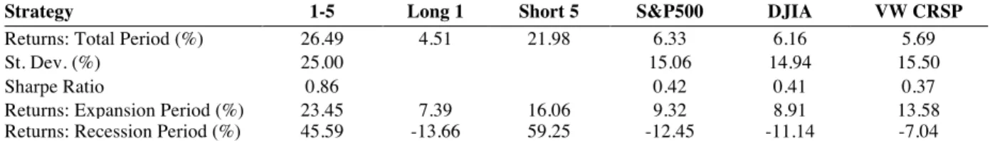
Moreover, there is a remarkable discrepancy of returns between recession and expansion periods in the 1-5 portfolio, at which the former clearly enlarge the outperformance of this strategy. This arises due to the short selling huge profits that account for the whole 1-5 return during recessions. When comparing the average annual indexes with the 1-5 portfolio returns on recession and expansion periods, it is clear that recessions are also driving the outperformance of our strategy, which we show in Table 3, below. The fact that our strategy is not only positive, but also much higher in recessions together with the short-selling high peaks in returns, allows it to benefit from the market losses. Therefore, this strategy constitutes a sustainable alternative in economic downturns.

Additionally, the 1-5 strategy gives us 0.86% returns per each percentage of risk taken (standard deviation) that is more than 50% higher than the Sharpe ratio (SR) obtained from any of the indexes. This is a good indicator regarding the risk-return relation of an investment, which, as it may be seen in

10 100 1,000 10,000 100,000 1,000,000 10,000,000 1963 1968 1973 1978 1983 1988 1993 1998 2003 2008 2012 SP500 Short 5 Long 1

(17)

Table 3, happens mostly due to the higher returns obtained together with relatively lower standard deviation of returns (from around 15% of the indexes to 25% of the strategy) in the 1-5 portfolio.

Table 3

Recession vs expansion periods

In the table we report the total period average annual returns, as well as, in recession and expansion periods of the 1-5 strategy, S&P500, DJIA and VW CRSP. We also show the returns on the two positions taken (long portfolio 1 and short portfolio 2), in order to analyze what are the main causes that explain the large outperformance of the 1-5 strategy. We show the Sharpe ratios of the 1-5 portfolio and the indexes, and the annualized standard deviation of each returns’, for a better understanding of the SR’s values. The sample is period is from February 1963 to December 2012.

4.2. Time-series regressions

We run time-series regressions over the returns of portfolios 1 to 5, as it follows,

𝑟_!,!= 𝛼_!,!+ 𝛽_!,! 𝑀𝐾𝑇 + 𝑠_!,! 𝑆𝑀𝐵 + ℎ_!,! 𝐻𝑀𝐿 + 𝑢_!,! 𝑈𝑀𝐷 + 𝑤_!,! 𝑊𝑀𝐿 + 𝜀_!,! (3)

In a first stage, we regress monthly excess returns with respect to the FF-3 factors, in order to evaluate the average returns in each portfolio (alpha) after controlling for the market, size and value factors. The objective is to check the signal and significance of alpha of the portfolio 5-1, in order to corroborate the profitability of the investment strategy described previously. Table 4 provides the time-series results of each quintile portfolio (1-Low to 5-High) on past IVOL and the portfolio 5-1. Panel A shows descriptive statistics for each portfolio. The average monthly returns span from 0.4% to -1.8%, in portfolio 1 and 5 respectively, confirming the decreasing returns trend from the bottom IVOL portfolio to the top one. The portfolios have around 800 stocks each, exhibiting the diversity and consistency of our sample with such large portfolios. The IVOL varies from 14% to 89%, on average, with a minimum of around 2% in the bottom portfolio and maximum of 503% in the top portfolio. The market capitalization mean of the portfolios’ firms is as large as 3,238 million dollars in portfolio 1, corresponding to 57% of the total sample, and 113 million dollars in portfolio 5, that is 2% of the total sample market capitalization.In Panel B of Table 4, we report the results for the five portfolios’ time-series regressions and the 5-1 portfolio, both equally and value weighted. We show the values of the intercept of each regression as

Strategy 1-5 Long 1 Short 5 S&P500 DJIA VW CRSP

Returns: Total Period (%) 26.49 4.51 21.98 6.33 6.16 5.69

St. Dev. (%) 25.00 15.06 14.94 15.50

Sharpe Ratio 0.86 0.42 0.41 0.37

Returns: Expansion Period (%) 23.45 7.39 16.06 9.32 8.91 13.58

(18)

well as the Newey-West adjusted t-statistics (computed with 5 lags) and the adjusted R2_{’s. As it may be}

seen, the alphas decrease monotonically from the first to the fifth portfolio and the adjusted R2_{’s are as}

high as 90%. The 5-1 portfolio coefficient is the most important to analyze, since it represents the returns’ difference between the top and the bottom monthly portfolios. Both equally and value weighted portfolios present negative 5-1 alphas that are negatively statistically significant at a 5% significance level, suggesting that the IVOL strategy of going long on the low IVOL stocks and short on the high IVOL stocks is profitable.

Table 4

Descriptive Statistics and FF-3 alphas on IVOL portfolios

The table shows descriptive statistics for the five IVOL sorted portfolios in Panel A. The row “% Market Cap” reports the percentage of the size of the whole sample that corresponds to each of the portfolios. In Panel B we show the alphas of the time-series FF-3 regressions for each portfolio and for the 5-1 portfolio, in percentage, as well as the robust t-stats in square brackets, below. The lines “Adjusted R2_{” correspond to the time-series regressions’ R}2_{’s, also reported in percentage.}

Considering the results obtained that prove the existence of the LVA among the U.S. stock market when controlling for the FF-3 factors, we now show evidence of a change in this pattern by including price momentum controls, following HLRZ (2010). Firstly, a long-term momentum factor is added to the model, the Carhart (1997) fourth factor, in order to control for the effect already documented by Jegadeesh and Titman (1993, 2001 and 2011), among others. They find that the tendency of the performance of U.S. stocks during the following three to twelve months will be similar to the one

Panel A: Descriptive statistics

Portfolios Ranked on Idiosyncratic Volatility

1 Low 2 3 4 5 High 5-1 VW Monthly Returns (%) 0.376 0.281 0.168 -0.511 -1.832 -2.208 EW Monthly Returns (%) 0.393 0.420 0.215 -0.240 -1.094 -1.488 # Stocks 812 812 812 812 812 Min IVOL (%) 1.9 19.9 28.8 40.0 58.4 Max IVOL (%) 19.9 28.8 40.0 58.3 503.5 Mean IVOL (%) 14.3 24.3 34.1 48.1 89.3 Market Cap (M) 3,238 1,373 624 301 113 % Market Cap 57.3 24.3 11.0 5.3 2.0

Panel B: Time-series FF-3 regressions alphas (%)

1 Low 2 3 4 5 High 5-1 Value Weighted -0.045 -0.274 -0.457 -1.250 -2.714 -2.669 [-1.05] [-4.28] [-5.35] [-8.35] [-14.02] [-12.67] Adjusted R2 ₉₄ ₉₅ ₉₃ ₈₈ ₈₁ ₆₁ Equally Weighted -0.211 -0.328 -0.598 -1.126 -2.067 -1.856 [-2.81] [-4.14] [-7.04] [-10.73] [-12.86] [-10.88] Adjusted R2 ₈₉ ₉₃ ₉₄ ₉₂ ₈₀ ₅₄

(19)

observed in the previous correspondent period, suggesting a persistence in time of stocks’ returns path. Therefore, we use the UMD factor that controls for the past 12-months returns as of the portfolio’s formation period (t-1). On the other hand, it is also shown in previous studies a strong effect in expected returns caused by prior short-term returns. The short-term return reversals is a well-established phenomenon according to Jegadeesh (1990) and Da, Liu and Schaumburg (2013), from which the profits are proof that market prices may reflect investor’s overreaction to information (called sentiment) or positions in illiquid stocks (called price pressure). This way, we construct another momentum factor, the past winners minus losers (WML), that takes into account the past 1-month returns as of the portfolio’s formation, according to HLRZ (2010). More specifically, in the t-1 period (IVOL portfolios formation), we rank monthly stocks by the previous month returns, forming ten past 1-month returns portfolios. We subtract the first decile portfolio equally average returns to the tenth one (past winners minus past losers) and thus have our WML factor.4 _{Hence, we are able to control for both long- and}

short-term price momentum effects, respectively, with the UMD and WML factors. Accordingly, we perform Equation (3) but using, from now on, the monthly returns of the 5-1 portfolio with respect to the FF-3 factors (Regression 1) plus the UMD and the WML factors (Regression 2 and Regression 3, respectively). Regression 4 corresponds to the entire Equation (3). In Table 5, we report the results for Regressions 1, 2, 3 and 4. We show the results for value and equally weighted portfolios (VW and EW, hereafter), accordingly in Panel A and Panel B. The alphas are statistically significant at a 5% significance level for all the regressions, except for Regression 3, but as we introduce the short-term momentum factor (in that regression), they switch from negative to positive. The coefficients from MKT, SMB and HML present all statistically significant values, showing the explanatory power of market returns, size and value on the 5-1 portfolio, whereas the MKT and SMB are always positive, indicating the outperformance of small stocks over large stocks and the HML is negative, as low book-to-market stocks outperform high book-book-to-market stocks, in the 5-1 portfolio.

4_{According to HLRZ (2010), the use of value-weighted returns in the creation of WML factor outcomes similar results to an equally weighted} average. Therefore we follow their methodology and used the value-weighted scheme for the factor computation. For more detailed information on the WML factor construction see HLRZ (2010).

(20)

Table 5

Long-Short portfolio time-series regressions

The table reports the time-series regressions coefficients, for the sample period February 1963 to December 2012. The dependent variable is the return from the 5-1 portfolio, in order to show the difference in returns between the top IVOL portfolio and the bottom IVOL portfolio. Robust t-stats are shown in square brackets, according to Newey-West (1987), adjusted for 5-lag residuals’ serial correlation. The lines “Adjusted R2_{” correspond to the time-series regressions’ R}2_{’s, also}

reported in percentage.

Also, since all the momentum factors’ coefficients are negatively statistically significant, we can assert that the 5-1 portfolio monthly returns are negatively affected by past returns, experiencing both long- and short-term return reversals. This way, we can conclude that the long-term return reversals effect did not explain the LVA; on the contrary, the short-term return reversals affected the 5-1 portfolio returns, which turned positive. Furthermore, by looking at the adjusted R2_{’s of the regressions we confirm the}

high global significance of the models performed, with values as high as 54% to 67%, and always increasing when adding the momentum factors, confirming exactly these factors’ explanatory power on the portfolio returns.

Panel A: Value Weighted time-series regressions

Regression Models Intercept (%) MKT SMB HML UMD WML Adjusted R2

Regression 1 -2.67 0.478 1.365 -0.298 61 [-12.67] [5.44] [51.98] [-2.59] Regression 2 -2.40 0.425 1.370 -0.390 -0.301 64 [-11.47] [5.80] [13.82] [-2.19] [-3.33] Regression 3 1.70 0.478 1.375 -0.302 -0.090 64 [1.54] [5.87] [17.84] [-2.80] [-3.70] Regression 4 2.38 0.421 1.380 -0.402 -0.326 -0.098 67 [2.31] [6.54] [14.96] [-2.56] [-3.36] [-4.41] Panel B: Equally Weighted time-series regressions

Regression Models Intercept (%) MKT SMB HML UMD WML Adjusted R2

Regression 1 -1.86 0.372 1.119 -0.246 54 [-10.88] [6.76] [15.00] [-2.53] Regression 2 -1.63 0.326 1.122 -0.326 -0.261 57 [-9.19] [6.87] [13.63] [-1.95] [-2.72] Regression 3 0.77 0.372 1.124 -0.248 -0.054 55 [1.20] [6.99] [15.38] [-1.64] [-2.45] Regression 4 1.35 0.324 1.129 -0.333 -0.276 -0.061 58 [2.08] [7.08] [13.96] [-2.12] [-2.77] [-2.74]

(21)

5. Portfolio analysis within industry segmentation

In this section, we perform an industry-specific analysis on the LVA. The motivation for this detailed analysis arises since, according to Chou et al. (2012), not only have industries not received the deep investigation they should among the academia papers, but also due to the existing relation between industry-related patterns and asset pricing theories. Besides, they prove that there is high comovement among firms from the same industry, confirming how industry-related patters have an impact in stock returns. So, what drives such within-industry comovements? They defend that either rational factors such as the common fundamentals shared by companies in the same industry, or behavioral forces like investors’ sentiment, might, at least partially, account for that. They find that industry returns cannot be totally explained by specific rational or behavioral theories, concluding that asset pricing anomalies shall not be attributed to isolated factors, such as industry segmentation. Motivated by these findings, we expect that by exploring within-industry returns the LVA might be strengthened, increasing investors’ potential profits when exploiting the 1-5 investment strategy.

Additionally, Hong et al. (2007) assert that many specific industries present similar patterns that predict the stock market. Also, they find a strong correlation between the stock market forecast power and the fact that industry returns foresee measures of economic activity, focusing on the industrial production growth. Moreover, they study the lead-lag effect among the stock market and its delayed reaction concerning industry returns information, by controlling for industry stock price momentum. This way, we include in our industry analysis controls for two different momentum factors, taking into account this delayed price reaction of the stock market as a result of the released information on industry returns. Furthermore, Wang (2010) documents investigation on trends of industry-specific volatility, suggesting that there are two particular industries that aggregate the most important indicators that lead industry-specific volatilities. Mostly important, they study volatility shocks in the stock market and find that three particular industries are the main sources of risk affecting many other industries. Nevertheless, further analyses have been developed concerning time-varying volatility among industries. For instance, Zhang (2010) compares different theories to explain the change in the average return volatility trend before and after 2000 and find that it is the average idiosyncratic volatility that has overall increased over time, while the market portfolio volatility does not appear to follow the same pattern. They show robustness

(22)

of these findings among different industries, and find different volatility patterns across industries using a 10-industry classification.

In this paper we focus on evaluating the persistence of the LVA across industries, in order to understand to which extent are there specific sectors where investors might achieve higher profits. In line with this, besides the controls for FF-3 factors, short- and long-term momentum factors are again taken into consideration due to their significant and strong explanatory power over stock returns across and within industries, as documented by Moskowitz and Grinblatt (1999). They explain that an investment strategy based on industry portfolios sorted on momentum (past winners minus past losers) is highly more profitable than the general momentum investment strategy of Jegadeesh and Titman (1993), since industry portfolios exhibit significant price momentum effect even after controlling for FF-3 and other risk factors. On the contrary, Hameed and Mian (2012) show that not only do intra-industry monthly returns evidence short-term reversals but also that these are larger in magnitude, persistent over time and more consistent across larger and more liquid stocks. Moreover, it is shown by Boni and Womack (2006) that the predictability of future relative under- and outperforming stocks within industries can be successfully drawn from changes in analyst recommendations. Also, they find that when controlling for price momentum within industry portfolios sorted on analyst coverage (leading to “hot” and “cold” industries), the factor loadings are remarkably lower relative to a non-recommendations analysis. Having this said, the point we raise is whether the industry segmentation will let us understand how can investors take better advantage from the LVA. Therefore, we apply the same methodology described in Section 4, by computing time-series regressions with respect to the portfolio 5-1 excess returns for two different industries’ segmentations. The industries’ classification is based on the Kenneth French data library definition, using the four-digit SIC codes. In a first stage we analyze 10 industries, although achieving inconclusive results as we explain in the following section. Hence we provide a 49-industry analysis afterwards. In Table 6, we present descriptive statistics concerning the 49-industry segmentation. The average number of months reported is different among industries, depending on the data available, which is filtered in order to have a minimum of 15 stocks per IVOL portfolio each month. The industries’ size varies from 39 to 3,363 million and the book-to-market ratios span from 0.35 to 2.81, showing the large disparity of size and value among industries.

(23)

Table 6

Descriptive statistics across industries

The table shows descriptive statistics regarding the 49-industry segmentation. The number of months changes across industries depending on the data available. We define a minimum average “# stocks” of 15 per portfolio, per month. All the remaining columns correspond to time-series averages of the variables concerning each specific industry.

5.1. Time-series evidence on IVOL Portfolio among 10 industries

We now perform the four regressions explained in Section 4.2 concerning a 10-industry classification. By looking at Figure 6, we report the results for Regression 1 in the dark grey bars, always considering a significance level of 5%. We find that all 10 industries have negative and significant values for the average monthly returns (alpha), which means that the 1-5 strategy is profitable for all industries, after controlling for the FF-3 factors. Thus, we confirm that among 10-industry market segmentation the LVA is persistent. Moreover, the adjusted R2_{is computed for each industry with values spanning from}

18% to 47%, suggesting a good global significance of the FF-3 model. The light grey bars show Regression 2 results, where we regress within-industry firm excess returns with respect to the four-factor model of Carhart (1997). Noticing the UMD effect, we clearly see two different clusters of industries: # Months Returns (%) # Stocks IVOL (%) Total Vol. (%) Mkt Cap (M) B/M

Food Products 323 0.14 17 39.0 43.7 717 1.04 Entertainment 165 -2.21 19 72.0 80.8 956 0.74 Consumer Goods 361 -0.13 21 41.5 46.9 783 0.95 Clothes 300 -0.47 17 45.7 50.6 137 1.79 Healthcare 304 -0.81 22 58.4 65.6 610 0.39 Medical Equipment 379 -0.77 30 55.5 63.0 1,107 0.46 Pharmaceutical 358 -0.54 45 57.9 66.4 2,682 0.35 Chemicals 440 -0.09 18 40.8 47.2 1,322 1.00 Textiles 416 -1.10 15 47.6 53.1 39 2.81 Construction Materials 416 -0.33 28 40.8 46.0 297 0.99 Construction 57 -0.73 16 59.7 66.4 164 1.08 Steel Works 367 -0.38 17 36.1 41.4 319 1.37 Machinery 572 -0.04 32 40.5 47.7 1,667 1.07 Electrical Equipment 288 -1.24 26 59.0 66.5 334 0.70

Automobiles and Trucks 323 -0.31 17 42.5 48.1 1,124 1.11

Oil and Gas 514 -0.15 38 48.0 55.9 2,585 0.79

Utilities 599 0.06 30 20.7 24.5 1,681 1.06 Telecom 355 -0.64 27 49.2 57.4 3,252 0.92 Personal Services 33 -0.33 16 57.2 64.3 435 0.49 Business Services 479 -0.62 53 51.0 58.4 505 0.79 Computer Hardware 409 -0.83 26 57.9 66.6 2,166 0.59 Computer Software 359 -0.70 56 59.3 68.5 1,614 0.48 Electronic Equipment 533 -0.49 45 51.9 60.6 1,127 0.78 Lab Equipment 429 -0.34 21 51.1 58.3 432 0.82 Transportation 455 -0.08 21 41.7 48.7 984 1.55 Wholesale 479 -0.42 38 47.7 54.5 491 1.01 Retail 581 -0.01 46 40.5 47.0 1,496 1.10

Restaurants and Hotels 431 -0.50 22 47.5 54.2 623 0.88

Banking 479 -0.09 73 32.2 37.6 990 1.18

Insurance 337 0.09 29 33.4 40.2 3,363 1.04

(24)

industries that provide products or services of essential needs and industries supplying other goods. The UMD is not significantly different from zero for the industries Durable Goods, Energy, Health and Utilities (the first cluster), whereas the companies trading in the second cluster (High Tech, Telecoms, Shops, Manufacturing and Non-dur. Goods) exhibit the opposite. This leads us to the conclusion that the companies providing essential goods do not experience long-term return reversals, hence tend to be more stable in terms of price variations than the second cluster, at which there are long-term return reversals. Moreover, the constant term remains significantly negative for all the industries, highlighting that the long-term return reversals do not explain the LVA. In the gold bars, the results correspond to Regression 3, where we include the Winners minus Losers factor (WML). Although the variable WML turns the average returns positive in all industries, they are never significantly different from zero, implying that the LVA disappeared. A similar industries’ clustering happens in what it concerns the impact of short-term momentum, strengthening our hypothesis that companies providing essential goods do not experiment return reversals, either long- or short-term. The fact that the 5-1 portfolio returns cease to be statistically different from zero suggests that, for the cluster experiencing return reversals, these totally explained the LVA.

Figure 6

10-Industry High-Low IVOL portfolio regressions

The figure shows the coefficients from the 4 regression models with the 5-1 portfolio returns. The bars dark grey, light grey, gold and dark blue report the results of Regression 1, 2, 3 and 4, respectively. The bars show the alpha value of each regression. The 5% significance or not of the alphas is represented by the existence or not of a dashed line around the bars, respectively. T-stats are adjusted for the regressions’ standard errors heteroskedasticity and serial correlation of 5 lags, following Newey-West (1987). Adjusted R2_{’s are shown on the right-hand side of the respective bars, with respect to each time-series regression.}

0.14 0.48 1.60 0.75 1.02 -0.30 0.41 1.02 0.44 0.47 -2.69 -2.54 -1.87 -2.17 -2.67 -2.87 -2.56 -2.11 -2.29 -2.89 46 21 47 18 34 44 22 44 19 32 45 21 45 19 32 43 21 42 18 31 High Tech Energy Mafufact Dur Goods ND Goods 2.68 0.98 -0.12 0.79 4.78 2.26 0.77 -0.58 0.07 3.28 -2.23 -0.51 -2.99 -2.79 -2.23 -2.38 -0.60 -3.15 -3.09 -2.66 49 18 49 42 37 47 18 48 38 34 45 18 48 40 37 44 18 47 37 33 Other Utilities Health Shops Telecom

(25)

In the dark blue bars, we test the two momentum factors together, regressing firm excess returns with respect to the FF-3 factors, UMD and WML (Regression 4). We find that the industries Telecoms and Others (that includes Finance, Hotels and Transportation sectors) are affected by both short- and long-term return reversals and have significantly positive 5-1 portfolio returns, indicating that a 5-1 investment strategy is beneficial. All the other industries appear to not experience the LVA, by having 5-1 portfolio returns statistically close to zero, either presenting or not return reversals. Corroborating the return reversals evidenced, Hameed & Mian (2012) also find that short-term return reversals are more present within industries and that momentum is more present across industries.

5.2. Time-series evidence on IVOL Portfolio among 49 industries

In this section, following the intuition mentioned before and given the similarity of the results obtained on the 10-industry analysis to the global market analysis, the main goal is to check whether the LVA persists in any industry and, if so, the 1-5 strategy outperforms the market, with a finer grid of industry segmentation, as of 49 industries. When taking into account the whole returns data sample for all the industries, in order to create the IVOL portfolios for each industry, a minimum number of stocks of 15 is defined as the limit for the portfolio formation. This way, only 31 industries turn out to have data available for the analysis. We run Equation (4) for each time-series of 5-1 portfolio returns with respect to the FF-3 factors, across all industries (Regression 1). We find that, from the 31 industries studied, 2 industries (Textiles and Personal Services) do not appear to evidence any anomaly regarding IVOL, presenting a difference in returns between the fifth and first portfolios approximately zero. We always consider a significance level of 5%. In Figure 7, in the dark grey bars, we show the regressions’ coefficients and the non-significance of the alpha in both industries is clear. Consequently, we run Regression 2 over the 29 remaining industries in order to examine whether the LVA is still persistent when controlling for long-term momentum. We find a negative and significant UMD coefficient in 10 of these industries, meaning that they experiment long-term return reversals, where 9 present also a negative and significant intercept, as reported in the light grey bars. Those 9 industries are, thus, still exhibiting a negative relation between IVOL and excess returns, while in the other one (Automobiles

(26)

and Trucks industry) the IVOL effect ceases to exist. The remaining 19 industries, despite not experiencing a long-term momentum effect, still present the LVA (except for the Utilities).

Figure 7

49-Industry High-Low IVOL portfolio regressions

The figure shows the coefficients from the 4 regression models with the 5-1 portfolio returns. The bars dark grey, light grey, gold and dark blue report the results of Regression 1, 2, 3 and 4, respectively. The bars show the alpha value of each regression. The 5% significance or not of the alphas is represented by the existence or not of a dashed line around the bars, respectively. T-stats are adjusted for the regressions’ standard errors heteroskedasticity and serial correlation of 5 lags, following Newey-West (1987). Adjusted R2_{’s are shown on the right-hand side of the respective bars, with respect to each time-series regression.}

In the gold bars, we report the results for checking whether the negative IVOL effect on stocks’ returns is still persistent when controlling for a short-term momentum factor (WML), by performing Regression 3. We find a negative and significant WML coefficient in 8 of these industries, meaning that they experiment short-term return reversals, where 2 present also a significant but positive 5-1 portfolio returns (Business Services and Construction), suggesting that the IVOL effect ceases to exist and is totally explained by this reversals. For these two sectors, the profitable strategy to apply is then the 5-1 portfolio. The remaining 20 industries present returns non-significantly different from zero, which might

23.59 0.48 -6.60 2.16 -0.10 2.65 0.93 -2.36 -2.64 9.67 -4.48 22.59 0.41 -7.37 2.07 -0.55 1.38 -0.65 -1.72 -2.69 9.41 -4.38 -2.70 -2.37 -1.60 -1.50 -3.11 -3.34 -3.27 -3.29 -2.36 -6.32 -2.06 -2.81 -2.42 -1.51 -1.52 -3.22 -3.64 -3.60 -3.07 -2.40 -6.77 -2.01 12 29 51 10 51 18 17 14 26 11 51 13 29 52 11 51 18 18 14 26 12 51 13 29 53 11 52 23 20 15 26 13 55 15 29 53 11 52 18 18 15 26 13 56 Construction Construction Mat. Textiles Chemicals Pharmaceutical Medical Equip. Healthcare Clothes Consumer Goods Entertainment Food Products Regression 3 Regression 1 Regression 4 Regression 2 Alpha significant

2.15 5.36 6.62 3.03 3.91 0.94 -0.53 -1.54 0.02 1.47 -1.45 0.86 5.18 6.06 9.79 1.75 0.73 -0.70 -1.72 -0.26 0.87 -1.43 -3.08 -4.16 -2.71 -2.44 -2.90 -0.50 -2.83 -1.10 -3.84 -2.15 -1.40 -3.39 -4.24 -2.84 -1.38 -3.42 -0.58 -2.89 -1.60 -3.93 -2.37 -1.39 19 28 24 18 33 15 18 14 40 34 21 19 28 24 5 33 15 18 15 40 34 21 23 28 24 21 41 16 18 18 40 34 21 19 28 24 6 34 15 18 15 40 34 21 Computer Software Computer Hardware Business Services Personal Services Telecom Utilities Oil and Gas Automobiles Electrical Equip. Machinery Steel Works 4.79 -2.05 0.87 3.38 3.67 1.26 1.64 0.81 1.50 4.07 -2.81 0.55 2.70 2.83 -0.13 0.22 0.05 0.58 -2.07 -2.35 -1.79 -3.32 -2.39 -2.88 -1.75 -1.91 -1.99 -2.26 -2.52 -1.88 -3.69 -2.72 -3.29 -2.16 -2.11 -2.34 17 15 13 20 32 22 20 25 22 18 16 14 20 32 22 20 25 22 18 16 14 21 32 23 20 25 22 18 16 14 20 32 22 20 25 22 Trading Insurance Banking Rest. & Hotels Retail Wholesale Transportation Lab equipment Electronic Equip.

(27)

be explained by having included in the model a variable that does not explain those returns. The industry Food Products is the only one that, by not experiencing short-term momentum, still appears to have statistically significant and negative 5-1 returns, hence exhibiting the LVA. Moreover, we aim to understand the implication of controlling for both momentum factors in the time-series regressions. For that purpose, we run Regression 4 among the 29 industries in order to assess the significance of these two new variables together and their impact on portfolio 5-1 returns, as shown in the dark blue bars of Figure 7. We find negative and significant UMD and WML coefficients in 9 of these industries, meaning that they experiment both short- and long-term return reversals, where 2 present also a significant intercept (Business Services and Retail industries). These industries shifted to positive returns in the 5-1 portfolio, suggesting that the momentum effects totally explained the existing LVA. Furthermore, the Construction and Computer Hardware industries also present significantly positive returns, even though not exhibiting long-term momentum in returns, leading to the same conclusion that a 5-1 strategy is the profitable one. On the other hand, again the Food Products industry appears to show neither short- nor long-term momentum, while still evidencing a negative and statistically significantly different from zero 5-1 portfolio return. This way, the 1-5 portfolio investment strategy is still profitable within this industry. Overall what we find is that the industry Food Products (FP hereafter) has a negative and large alpha (-4.5%), even after controlling for five risk factors, which does not happen in any of the analyses performed before.

As a result, we now show a more detailed analysis concerning this specific industry. In Table 7, we report descriptive statistics of this industry and of the average regarding all the other industries (IA from now on), in order to make a comparison in terms of what characterizes the former against to the remaining average. The average number of firms in FP is almost half of the observed in IA, but the size of the sample (“# months”) is not much smaller, with returns spanning from February 1973 to December 1999. The average monthly return is positive in the FP, which does not verify in the IA and both the total volatility and IVOL are larger in the latter. The average size is considerably smaller in the FP and the book-to-market ratio appears to be higher, yet these are not so comparable between the two sets since the samples are different.

(28)

Table 7

Comparison of the Food Products industry with the remaining industries

The sample size for the Food Products industry is from January 1973 to December 1999. The “Overall” sample size for All industries is an average of the number of months in the data available for each of the industries, excluding FP. The remaining descriptive statistics are equally weighted averages of the time-series data.

Accordingly, the 1-5 portfolio strategy described before seems to be profitable applied to the FP industry. In Figure 8 we show the outperformance of the FP 1-5 portfolio returns over the S&P500, Dow Jones Industry Average (DJIA) and value weighted CRSP indexes returns, evidencing the large returns obtained from the LVA investment strategy.

Figure 8

Comparison of the Food Products industry with the indexes

The figure shows the monthly value of the Food Products industry 1-5 portfolio, the S&P500, the DJIA and the VW CRSP indexes based in January 1973 with a value of $100, with the returns spanning from February 1973 to December 1999. The grey bars correspond to the recession periods, according to the NBER.

Descriptive statistics Panel A: Food Products industry

IVOL portfolios 1 Low 2 3 4 5 High 5-1 Overall

# Months 323 Monthly Returns (%) 0.78 0.51 0.44 0.11 -1.13 -1.91 0.14 # Stocks 17 17 17 17 17 17 Min IVOL (%) 3.9 18.6 26.4 37.0 55.2 28.2 Max IVOL (%) 18.2 26.0 36.1 53.6 178.2 62.4 Average IVOL (%) 13.3 22.2 30.9 44.5 84.1 39.0

Average Total Vol. (%) 24.3 29.6 37.4 49.3 77.9 43.7

Market Cap (M) 1,937 1,069 387 152 41 717

% Market Cap 54.0 29.8 10.8 4.2 1.1

Book-to-Market 0.95 0.99 1.09 1.20 1.00 1.04

Panel B: All industries

# Months 390 Monthly Returns (%) 0.40 0.26 -0.09 -0.90 -2.05 -2.45 -0.48 # Stocks 30 30 30 30 30 30 Min IVOL (%) 6.2 24.0 33.6 45.4 65.4 34.9 Max IVOL (%) 23.6 33.2 44.8 64.2 233.5 79.9 Average IVOL (%) 17.4 28.6 38.9 53.7 98.6 47.4

Average Total Vol. (%) 28.4 37.1 49.2 60.6 95.8 54.2

Market Cap (M) 3,361 1,310 674 339 137 1,164 % Market Cap 57.7 22.5 11.6 5.8 2.3 Book-to-Market 0.97 0.93 0.91 0.92 0.89 0.93 1 10 100 1,000 10,000 100,000 1973 1976 1979 1982 1985 1988 1991 1994 1997 SP500 DJIA FP 1-5 VW CRSP index

(29)

In Table 8, we report the average annual returns from the 1-5 FP strategy as well as the three indexes returns, for the total period from February 1973 to December 1999, and for recession and expansion periods. We find that this strategy is more profitable during expansion periods, evidencing larger returns, and that what mostly drives them is the short position in the fifth portfolio. Additionally, the strategy presents recession positive average returns, while both indexes are negative in these periods. Moreover, the 1-5 FP strategy gives us 0.65% returns per each percentage of risk taken (standard deviation) that is higher than the Sharpe ratio (SR) obtained from any of the indexes. This is a good indicator regarding the risk-return relation of an investment, which, as it may be seen in Table 8, happens mostly due to the higher returns obtained together with relatively lower standard deviation of returns (from around 15.8% of the indexes to 25% of the strategy) in the 1-5 FP portfolio.

Table 8

1-5 Food Products: Expansion vs Recession

In the table we report the total period average annual returns, as well as, in recession and expansion periods of the 1-5 Food Products industry strategy, S&P500, DJIA and VW CRSP. We also show the returns on the two positions taken (long portfolio 1 and short portfolio 2), in order to analyze what are the main causes that explain the large outperformance of the 1-5 FP strategy. We show the Sharpe ratios of the 1-5 FP portfolio and the indexes, and the annualized standard deviation of each returns’, for a better understanding of the SR’s values. The sample is period is from February 1973 to December 1999.

Strategy FP 1-5 Long 1 Short 5 S&P500 Dow Jones VW CRSP

Returns: Total Period (%) 22.92 9.35 13.57 9.14 8.84 13.82

St. Dev. (%) 25.04 15.60 15.86 15.91

Sharpe Ratio 0.65 0.59 0.56 0.45

Returns: Expansion Period (%) 23.34 9.48 13.87 11.46 11.23 15.99

Is the low volatility anomaly still persistent? : it depends!