Duarte Gonçalves Galhardo
Bachelor of Science in Environmental Engineering
Tools to Predict Road Runoff Pollution
Dissertation to obtain Master Degree in Environmental Engineering
Supervisor: João Nuno Fernandes, Postdoctoral Research Fellow, LNEC
Co-Supervisor: Pedro Santos Coelho, Assistant Professor, FCT NOVA
Jury:
President: Leonor Miranda Amaral, Assistant Professor, FCT NOVA
Examiner: Ana Estela Barbosa, Assistant Researcher, LNEC
Supervisor: João Nuno Fernandes, Postdoctoral Research Fellow, LNEC
December, 2018
iv
Duarte Gonçalves Galhardo
Bachelor of Science in Environmental Engineering
Tools to Predict Road Runoff Pollution
Dissertation to obtain the Master’s Degree in Environmental Engineering
Supervisor: João Nuno Fernandes, Postdoctoral Research Fellow, LNEC
Co-Supervisor: Pedro Santos Coelho, Assistant Professor, FCT NOVA
Jury:
President: Leonor Miranda Amaral, Assistant Professor, FCT NOVA
Examiner: Ana Estela Barbosa, Assistant Researcher, LNEC
Supervisor: João Nuno Fernandes, Postdoctoral Research Fellow, LNEC
Faculty of Sciences and Technology NOVA University of Lisbon
v Tools to Predict Road Runoff Pollution
© Copyright, 2018, Duarte Gonçalves Galhardo, Faculdade de Ciências e Tecnologia e Universidade Nova de Lisboa. All rights reserved.
The Faculty of Science and Technology and NOVA University of Lisbon has the right, forever and without geographical limits, to file and publish this dissertation through printed copies reproduced in paper or in digital form, or by any other means known or to be invented, and to disseminate it through scientific repositories, and to permit its copying and distribution for non-commercial educational or research purposes, provided the author and publisher are credited.
vii
Agradecimentos
Este trabalho representa o culminar dos últimos cinco anos da minha vida. Resta-me agradecer, desta forma singela, às pessoas que nele estiveram presente com quem tive não só o prazer trabalhar mas também de criar amizades.
Ao Laboratório Nacional de Engenharia Civil (LNEC), pela oportunidade de integrar um grupo e uma instituição tão prestigiada e que tanto me ensinou neste período.
Ao Engenheiro João Fernandes, pela orientação de trabalho ao longo deste tempo, mas também pela amizade e forma como me acolheu nesta etapa da minha vida.
Ao Professor Pedro, por me ter dado esta oportunidade, mas também por aquilo que representou ao longo do curso. Mais do que um Professor, uma ajuda constante e sempre disponível para ouvir. Quaisquer palavras ficarão aquém. Obrigado por tudo!
À Engenheira Ana Estela Barbosa, pela oportunidade de desenvolver o meu trabalho no âmbito de um projeto tão interessante.
Ao grupo de colegas do LNEC, pelo companheirismo e motivação ao longo de todos estes meses.
À minha família, por serem imprescindíveis. Vocês sabem o quanto são valiosos e o quanto a minha vida se baseia em tudo aquilo que me ensinaram e ensinam dia a dia. Nada disto era possível, nem valeria a pena sem vocês. São tudo para mim!
À Sara, por mais do que uma ajuda constante nesta tese, me aturar no último ano. Obrigado por estares sempre ao meu lado e seres a minha maior confidente e melhor amiga.
À Pipa, ao Marco, à Bela e ao Zé Duarte, pela amizade e apoio nesta fase da minha vida.
Aos meus amigos de Arraiolos por estarem presentes mesmo após largos meses de ausência.
Aos amigos que a grande FCT me deu. Esta faculdade só se tornou tão grande e tão especial na minha vida, hoje e sempre, devido à vossa presença. Obrigado pela cumplicidade, pela amizade, pelas noites de estudo e por tudo aquilo que já vivemos e iremos viver, juntos.
ix
Abstract
The concern about the environment is constantly increasing. The conservation of water resources is among the major issues. If previously the major concern with this resource was only the quantitative level, nowadays the qualitative level is a concern equally important.
Taking into account this major concern and due to the increasing urban development, road runoff has become a growing issue since it is a potential form of diffuse pollution. Because of the relevance of this source of pollution, road operators and environmental agencies have developed new models for road runoff prediction. In this dissertation, four of these models were assessed: PREQUALE (Portugal), Highways Agency Water Risk Assessment Tool (HAWRAT - UK), Kayhanian’s model (USA) and Stochastic Empirical Loading and Dilution Model (SELDM - USA).
After a literature review on this subject, the study started with the collection of monitored data from 20 roads in six European countries. For each road, the Site Mean Concentrations (SMC) were calculated for total suspended solids (TSS), copper, zinc, lead and cadmium. From these the SMC of TSS were above the emission limit declared by the Portuguese regulation (Decree-Law 236/98, from 01 of August) for some of the roads.
The second step was the evaluation of the four prediction models, through the comparison between monitored data and model results. Together with the visual observation, four error indices were calculated to check which model was best adapted to the European monitored data. It was verified that none of the models presents sufficiently robust values to be used like a general model of application to the whole Europe.
Furthermore, a new prediction equation was developed. This equation was calibrated with data from all Europe, unlike the four previous models, which were calibrated for a country or region. As whole data were used to calibrate the model, the results agree with the data. Nevertheless, its use in real and different roads should be carefully assessed.
xi
Resumo
Os recursos hídricos têm apresentado cada vez maior importância, havendo uma transformação na consciência coletiva, sendo que inicialmente a importância deste recurso era essencialmente quantitativa e agora é igualmente qualitativa.
Tendo em conta este facto, as escorrências rodoviárias tornaram-se uma preocupação cada vez maior, visto constituírem uma potencial fonte de poluição difusa. Tendo em conta esta premissa, as agências rodoviárias e do ambiente têm desenvolvido novos modelos de previsão de escorrências rodoviárias. Neste trabalho foram estudados quatro modelos: PREQUALE (Portugal), Highways Agency Water Risk Assessment Tool (HAWRAT do Reino Unido), um modelo de Kayhanian (EUA) e Stochastic Empirical Loading and Dilution Model (SELDM dos EUA).
Primeiramente foram recolhidos dados monitorizados de 20 estradas de seis países europeus sendo posteriormente calculadas as concentrações médias do local (CML) para cada uma das estradas. Foi possível verificar que apenas a CML de sólidos suspensos totais para algumas estradas se encontra acima do limite de emissão de águas residuais consignado no Decreto-Lei n.º 236/98, de 01 de agosto, estabelecendo-se assim uma análise das CML a nível europeu.
Posteriormente, foi feita uma avaliação dos quatro modelos estudados. Para cada uma das 20 estradas foi estudado qual o modelo que melhor se adaptava aos resultados de monitorização, através de uma análise visual e de erros calculados. Verificou-se que nenhum dos modelos apresenta valores suficientemente robustos para ser utilizado como modelo geral de aplicação a toda a Europa.
Tendo a análise dos quatro modelos em conta, foi desenvolvida uma equação de previsão, que foi calibrada com os dados das 20 estradas europeias, ao contrário dos quatro modelos anteriormente referidos, que foram calibrados para um determinado país ou região desse país. Os resultados não foram considerados suficientemente robustos, para permitir a utilização deste modelo à escala europeia, mas foram bastante melhores que os obtidos através dos outros modelos, tendo em conta que o modelo foi aplicado às estradas que permitiram a sua calibração. O uso deste modelo em novas estradas deve ser objeto de uma análise bastante cuidada.
Palavras-Chave: Escorrências rodoviárias, PREQUALE, HAWRAT, modelo de Kayhanian, SELDM, CML.
xiii
List of Contents
1 Introduction ... 1
1.1 Road runoff pollution ... 1
1.2 Scope and objectives ... 1
1.3 Dissertation structure ... 3
2 Literature review ... 5
2.1 Road runoff pollution ... 5
Generic characterization of road runoff pollution ... 5
Pollutants and sources ... 7
Receiving waters impacts ... 9
Acute and cumulative impacts ... 9
Specific cases ... 10
Concentrations... 10
2.2 Tools to predict road runoff ... 11
3 Data and Methods ... 12
3.1 Data collection ... 12
3.2 Description of the models ... 14
PREQUALE ... 14
Highways Agency Water Risk Assessment Tool (HAWRAT) ... 16
Kayhanian’s multiple linear regression method ... 19
Stochastic Empirical Loading and Dilution Model (SELDM) ... 20
Inputs and outputs summary table ... 23
4 Assessment of the predicting tools ... 25
4.1 Methodology ... 25
4.2 Input Data ... 30
4.3 Comparison of the predictions ... 32
4.4 Critical review of the models ... 34
5 Proposed model ... 37
5.1 Development of a new model ... 37
5.2 Results and performance evaluation ... 38
xiv 6 Conclusions and further work ... 41 7 References ... 43 Annexes ... 49
xv
List of figures
Figure 1.1 – Representation of road runoff and probable ways of reaching surface water bodies... 2
Figure 2.1 – Example of first-flush effect ... 6
Figure 3.1 – Europe precipitation map with the roads under study ... 13
Figure 3.2 – HAWRAT methodological scheme ... 16
Figure 3.3 – Representative map of the limits/areas used in HAWRAT ... 18
Figure 3.4 – Mass balance for each storm event ... 21
Figure 3.5 – Stochastically generated rainfall events with Portuguese data ... 22
Figure 3.6 – Ordered stochastically generated rainfall event for the same site in Portugal ... 22
Figure 4.1 – SMC of each test performed in the sensitivity test ... 26
Figure 4.2 – Comparison of A25 results for monitored and predicted concentration through similar events ... 27
Figure 4.3 – Spreadsheet model to calculate model’s inputs ... 28
Figure 4.4 – Comparison SMC monitored and predicted (a) TSS; (b) copper; (c) zinc; (d) lead and (e) cadmium ... 32
Figure 5.1 – Comparison of the predicted and monitored data of (a) TSS; (b) Copper; (c) Zinc; (d) Lead and (e) Cadmium ... 38
xvii
List of tables
Table 2.1 – Main pollutants and associated sources ... 7
Table 2.2 – Road runoff components division ... 8
Table 2.3 – Main impacts per type of pollutants ... 9
Table 3.1 – Road characteristics ... 12
Table 3.2 – SMC of each site ... 13
Table 3.3 – Intervals for which PREQUALE had been validated ... 15
Table 3.4 – PREQUALE roads ... 15
Table 3.5 – PREQUALE regression and correlation coefficients ... 16
Table 3.6 – Constants table in order to predict concentrations trough HAWRAT ... 18
Table 3.7 – Constants Kayhanian’s model ... 20
Table 3.8 – Inputs summary table ... 23
Table 3.9 – Outputs summary table ... 24
Table 4.1 – Sensitivity SELDM test inputs ... 25
Table 4.2 – Physical characteristics of road used as inputs in the tools ... 30
Table 4.3 – Error indices table ... 33
Table 4.4 – Table regarding the pros and cons of each model ... 35
Table 5.1 – Correlation coefficients ... 37
xix
Acronyms and glossary
AADT Annual average daily traffic
AADTC Annual average daily traffic constant ADP Antecedent dry period
ANN Artificial neural network
AR Annual average rainfall volume with the same duration as the basin concentration BDF Basin development factor
Cp Estimated concentration for the pollutant p
COD Chemical oxygen demand
CR Climate region
CRC Climate region constant CRM Coefficient of residual mass CSR Cumulative seasonal rainfall
DA Drainage area
DL Drainage length
EMC Event mean concentration
ENS Efficiency Nash-Sutcliffe coefficient
GUI Graphical user interface
HAWRAT Highways Agency Water Risk Assessment Tool HRDB Highway Runoff Database
IDF (curves) Intensity-duration-frequency (curves)
IF Impervious fraction
MC Month constant
MHI Maximum hourly intensity MLR Multiple linear regression
Pannual Annual average rainfall
PAH Polycyclic aromatic hydrocarbon
PC Pollutant constant
PROPER Project Road Runoff Pollution Management and Mitigation of Environmental Risks R2 Coefficient of determination
RMSE Root mean square error
S Average slope
SELDM Stochastic Empirical Loading and Dilution Model SMC Site mean concentration
Tc Concentration time
TER Total event rainfall TSS Total suspended solids USA United States of America
1
1 Introduction
1.1
Road runoff pollution
In the context of the growing environmental concern worldwide, the quality of the water bodies is a major issue. Some management strategies to control nonpoint and point source pollution have been applied. One source of nonpoint pollution of these water bodies comes from road runoff, which may have much lower quality than the effluent of some wastewater treatment plants (Ringler, 2007). Thus, there is a need to study and provide better tools to support decision makers on the management of the quality of these water bodies. One of the most worrisome concerns at the national level is the lack of any specific legislation to evaluate this type of runoff. The Portuguese Decree-Law n.º 236/981, from 01
of August, which establishes quality standards, criteria and objectives for the purpose of protecting the aquatic environment and improving water quality in relation to its main uses is currently being used as legal framework to support the study of road runoff. It is important to notice that this Decree-Law is only used as a reference to the researchers, due to the fact that road runoff has very different characteristics than the rejected water from the wastewater treatment plants, for several reasons, such as: (i) the legislation is applicable only for punctual and not for diffuse pollution, which is the case of road runoff pollution and (ii) on road runoff, the seasonality is much more clear than in the waters from the wastewater treatment plants.
In response to the European environmental concern, the Water Framework Directive (OJEC, 2000) has emerged, which requires a good understanding of the impacts of pollution sources and also the control of the most relevant to the receiving water bodies. In the case of roads, Barbosa et al. (2011) argues that it is important that the assessment of concentrations and pollutant loads take into account the characteristics not only of the road, but also of the climate. The prediction of the quality of a road runoff is a rather challenging issue due to its stochastic and diffuse nature. Winkler (2005) states that, even more complicated is the ability to assess the impact of pollutants on the receptor medium due to the need to analyse the case over a large time scale (e.g. due to persistent substances).
In this dissertation, previously collected data of road runoff of six European countries were gathered and compared to the predictions of four models. In order to provide decision makers with the most reliable tools, an assessment of these models was performed. Moreover, a regression model intended to predict total suspended solids (TSS), copper, zinc, lead and cadmium site mean concentrations (SMC) was also developed using the data from six European countries.
1.2
Scope and objectives
The current work is part of an European research project, funded by the Conference of European Directors of the Roads, entitled Project Road Runoff Pollution Management and Mitigation of Environmental Risks (PROPER). It aims at reviewing and generating knowledge that can be used at European level. Several studies have been developed in this area in view of a greater environmental
1 In this dissertation, the norms of the Portuguese Decree-Law n.º 236/98 from 01 August considered were the
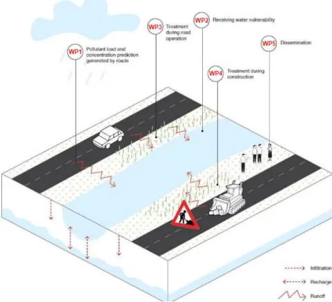
2 concern, having in this case a preponderance over water. The dissertation is included in the Work package 1 (cf. Figure 1.1).
The pollutants generated through the traffic and road construction and maintenance can be automatically deposited in the soil, or emitted into the air and subsequently, some of them, deposited due to gravitational force or precipitation reaching the closest surface water bodies, as indicated in Figure 1.1. Although the sources of pollutants in these infrastructures are well defined, literature indicates that the prediction of pollutant loads and concentrations is uncertain. This uncertainty is due to the several variables at stake, for instance, the type of pavement of the road, the antecedent climatic conditions and the intensity, frequency and magnitude of rainfall events. These must be viewed as a stochastic phenomenon as it is impossible or not realistic to determine the exact process boundary conditions (Fernandes and Barbosa, 2018).
Tools that apply to the understanding of pollutant sources, their mobilisation, transport to the receiving environment and groundwater, should be seen not in an exact context, but through a statistical or risk assessment (Fernandes and Barbosa, 2018).
Figure 1.1 – Representation of road runoff and probable ways of reaching surface water bodies (source: http://proper-cedr.eu/index.html)
The current work has the following main objectives:
(i) Characterisation of the road runoff in and European context; (ii) Collection and analysis of available monitored data;
3 (iii) The assessment of road runoff predicting tools (HAWRAT - Highways Agency Water Risk Assessment Tool; SELDM - Stochastic Empirical Loading and Dilution Model; PREQUALE and Kayhanian’s multiple linear regression method).
(iv) Development of a new SMC prediction model.
1.3
Dissertation structure
The dissertation is divided into six distinct chapters, the contents of which are summarised below. The present chapter presents the introduction and the objectives of the dissertation. In the second chapter, a review of the worldwide existing literature is presented, focusing essentially on the European references. This section corresponds to a generic characterisation of road runoff pollution, a description of the pollutants and corresponding sources and the distinction between acute and cumulative impacts. Moreover, specific cases like highways maintenance and accidental spillages, concentrations and loads calculations and a brief view of road runoff model types are presented.
The third chapter comprises the monitoring data collection for each country, its comparison with the legal regulated limits and the description of the predicting models that were assessed in the current work.
The fourth chapter concerns the assessment of the predicting tools. After a sensitivity test of a specific model, the methodology followed for the assessment is presented. Issues like the input data and the easiness of application are presented. Finally, a critical review is presented for each of the models, comparing their predictions with the monitoring data
The fifth chapter concerns the development of a new model. This model is the only model studied in this work that was calibrated with European data from more than one country.
5
2 Literature review
2.1
Road runoff pollution
Generic characterization of road runoff pollution
A shift of the main concern about water management from quantity to quality and quantity has been noticed. In addition to this concern, there was an attempt to ensure the integrated management of the resource in a perspective of strong sustainability, considering the technical, economic, social and ecological aspects (Coelho, 2009).
Several studies were developed to manage and preserve the water resources. The main difference that can be pointed out in relation to the possible inputs of pollutants into the receiving bodies concerns the distinction between point and nonpoint source or diffuse pollution. The first refers to a direct and easily identifiable input (e.g. a pipe) of a polluted effluent while nonpoint source pollution corresponds to an effluent input from various origins like superficial runoff, atmospherically deposition, precipitation or infiltration, which origin is hard or almost impossible to identify, as stated by Loague and Corwin (2005).
Road runoff is often seen as an effluent with well-defined characteristics. Still, it covers a complex matrix of pollutants mainly dependent on various factors such as traffic or the characteristics of the site where they are generated. Barbosa et al. (2011) highlights that the potential impact of these pollutants must be studied taking into account both pollutant and the receiving environment characteristics. The Water Research Council points out, in a report of 2002 (as cited in Higgins, 2006), that the base pollutant matrix of a road runoff water is composed of solids, metals, hydrocarbons and inorganic salts, as indicated in Table 2.1. All these pollutants, depending on their quantity and state, can have a detrimental impact on receiving surface and underground water bodies (Barret et al., 1995 in Higgins, 2006). The main anthropogenic sources that lead to the above-mentioned pollutant matrix are not only the circulation of vehicles on the highways and their maintenance as can be easily verified in CIRIA report of 1994 (in Higgins, 2006), but also road signs as indicated by Barbosa et al. (2011).
Road runoff is recognised as a nonpoint source pollution. Thus, there is a responsibility for the management operators and the national authorities to ensure that these discharges comply with their respective national legislation, which has been reinforced by the European Union Water Framework Directive (Barbosa et al., 2011). Since its implementation, there has been a greater need to define the source of pollutants affecting the receiving environment and the need for nonpoint source pollution management (OJEC, 2000 in Higgins, 2006). Therefore, improvements on water treatment strategies have been continuously developed.
Higgins (2006) pointed out the five main categories of factors affecting contaminant concentrations namely: (i) Traffic volume and characteristics; (ii) Precipitations characteristics and pattern; (iii) Surrounding land use; (iv) Pavement structure and material used in construction; (v) Pollutant characteristics.
Regarding the effects of the traffic volume in the road runoff pollution, at least three different ways of measuring traffic volume can be identified (Irish et al., 1995): (i) Vehicles travelling during the storm (VDS); (ii) Vehicles travelling in the antecedent dry period (VADP); (iii) Annual average daily traffic
6 The classification of traffic volume could be made in several ways. While many road agencies use AADT to determine whether or not a highway needs to have a treatment system for their runoff, there are several authors who have found no relationship between this indicator and the load and concentration of solid pollutants, heavy metals, oils and lubricants (Higgins, 2006). Irish et al. (1995) suggests that the number of vehicles traveling during a storm may be a significant factor in determining pollutant loads, since they are in direct contact with precipitation during a high rainfall event.
Regarding the precipitation characteristics, three main indicators are commonly found in literature to assess its influence in road runoff pollution, namely: (i) Antecedent dry period (ADP); (ii) Rainfall intensity; (iii) Runoff volume. ADP is defined as the period of time with no runoff (days or hours) preceding a storm event (Irish et al., 1995). An early research from Howell (1978) (in Irish et al., 1995) suggests that the preceding dry period was significant to the build-up of solids on the highway and the corresponding pollutant loads in the runoff. The rainfall intensity is a key factor in relation to the pollutant loadings because the rain is the main driving force in which contaminants are removed from the air, vehicles and the highway surface (UK Transport Research Laboratory, 2002).
The characteristics of precipitation are the most important for the occurrence of the so-called "First-Flush" effect. This phenomenon occurs when a precipitation event is preceded by an ADP of several days. During the beginning of the rain event, road runoff water pollution is typically more pollutant concentrated compared to the rest of the storm. The first-flush phenomenon is affected by certain parameters like the size of the watershed, rainfall intensity, impermeable area and the antecedent dry weather period. The concentration peak varies for each pollutant during the same rainfall event or in the same watershed during different rainfall events (Wanielista and Yousef, 1993 in Yannopoulos et al., 2013). The occurrence of a first-flush effect in a road runoff event is exemplified in Figure 2.1.
7 Pollutants and sources
Road traffic, weather conditions and the highways maintenance are responsible for the transport of the road runoff to the receiving environment (Piguet, 2007 and Kobriger and Geinepolos, 1984). The main pollutants comprise solids, heavy metals, inorganic salts and hydrocarbons. A list of pollutants and their sources are listed in Table 2.1.
Table 2.1 – Main pollutants and associated sources (Higgins, 2006)
Pollutant Specific Contaminant Source
Solids Carbon Organic Solids Rubber Plastic Grit Asbestos Rust Metal Filings Exhaust, Oil Oil, Exhaust Tyres Vehicles
Deicing salts, Road structure Brakes, Clutches Vehicles Vehicles Metals Arsenic Barium Cadmium Calcium Chromium Copper Iron Lead Magnesium Manganese Nickel Zinc Fuel Paints, Rubber
Tyres, Oils, Galvanised metals Oils, Deicing salts
Metal plating, Bearings, Brushings Paints
Tyres, Brakes, Oils, Bearings Corrosion
Fuel, Tyres, Brake linings, Bearings Cast metal
Tyres, Brakes, Oils, Bearings
Fuel, Paints, Tyres, Lubricants, Corrosion, Brakes
Hydrocarbons Aliphatic Hydrocarbons Poly Aromatic Hydrocarbon Phenols Carbonyl Compounds Bitumen Asphalt Solvents Polychlorinated biphenyl (PCB) Methyl tert-butyl ether (MTBE)
Lubricant, Fuel, Anti-freeze Fuel, Lubricants
Lubricants, Fuel, Anti-freeze Combustion products Road surface Road surface Spillages Fuel combustion Fuel combustion Fuel combustion Inorganic Salts Nitrates Chlorides Phosphates Herbicides Lubricating oil Deicing salts Lubricating oil
8 As not all the pollutants from runoff presented in Table 2.1 are regularly monitored, Kayhanian et al. (2012) suggested a selection of the most important parameters to be monitored to evaluate the road runoff (cf. Table 2.2).
Table 2.2 – Road runoff components division (Kayhanian et al., 2012) Runoff Components
Conventional and aggregate water quality parameter
TSS; Total dissolved solids; Dissolved organic carbon; Total organic carbon; Chemical oxygen demand (COD); Biochemical oxygen demand; Oil and
grease; Hardness as CaCO3; Temperature; pH
Metal constituents
Most frequently: Cadmium; Chromium; Copper; Lead; Nickel; Zinc Less frequently: Aluminium; Arsenic; Iron
Nutrient constituents *Nitrates; Ammonium; Total Kjeldhal nitrogen; Total nitrogen; Total
phosphorus Infrequently measured water
quality parameters
Fecal indicator bacteria; Toxicity; Polycyclic aromatic hydrocarbons (PAHs); Herbicides; Pesticides
*Kayhanian et al. (2012) also points out that the presence of phosphorus and nitrogen as pollutants in the monitoring of runoff water is due not only to pollutant sources related to road traffic, but also due to external factors.
The mentioned pollutants are not only caused by road traffic. They may come from several sources, both anthropogenic and natural. Some are transported long distances by the wind, being deposited later in the most varied places as stated by Fritzer (in Winkler, 2005). According to the same source, the most relevant related pollution sources are: the abrasion of road surfaces; the abrasion of tires; drip loss; combustion emission; the abrasion of brake pads and clutch plates.
After considering road traffic and emitted pollutants into the atmosphere as the first and second source of road pollution, Barbosa et al. (2011) pointed out the maintenance and construction activities as a third source of pollutants. As far as construction is concerned, the largest pollutants are related to solids and accidental cases, such as situations with fuels, oils and lubricants. Regarding the road maintenance, the main sources of pollutants are the de-icing salts (chlorides) used in some parts of Europe, where snow and ice abound during the colder periods of the year, as well as herbicides, which in high concentrations lead them to be a persistent pollutant in the ecosystem (Mudge and Ellis, 2001 in Higgins, 2006).
9 Receiving waters impacts
The potential impacts of each pollutant in the receiving water are presented in Table 2.3. Table 2.3 – Main impacts per type of pollutants
Pollutant Impacts
Solids
Reduce light transmission which limits photosynthesis and diminishes aquatic food supply (Goldman, 1986 and Barret et al., 1995 in Winkler, 2005);
Lead to an elevated level of insoluble substances with negative impacts on fish eggs and larvae trough clogging of the pores between the substrate of the riverbed (Winkler, 2005); Clog fish gills and harm their respiration and the respiration of other aquatic animals (Hill, 2010).
Metals
Can be toxic because metals undergo bioconcentration (Salomon, 2008).
The toxicity associated may reduce diversity and abundance of the sensitive aquatic biota and replace them with pollution tolerant species (Hvitved-Jacobsen and Yousef, 1991); Copper, cadmium and zinc could be toxic even in low concentrations (Scheffer and Schachtschabel, 2002 and Hahn, 2004 in Winkler, 2005).
Hydrocarbons
Several PAHs are toxic, mutagenic/carcinogenic. This type of pollutants is highly lipid soluble and thus easily absorbed by human bodies (Abdel-Shafy and Mansour, 2015). Methyl-Tertiary-Butyl-Ether (MTBE) is toxic to several freshwater organisms (Werner et al., 2001).
Inorganic Salts
Like fertilizers and herbicides, used in the maintenance of road shoulders, essentially on the roadside, lead to an increase in phosphorus and nitrogen in the runoff matrix, which contributes to the eutrophication of the receiving environment (Hvitved-Jacobsen and Yousef,1991).
Acute and cumulative impacts
Depending on the pollutant type, concentration, rate of assimilation of organisms, and on its form (dissolved and particulate), the impacts created in the water environment may be acute or cumulative. Acute effects are associated with accidental spills and/or organic or metallic pollutants entering the composition of road runoff. Other examples of acute effects are the presence of copper in its soluble form, soluble short-chain organic pollutants (e.g. herbicides) and runoff of suspended solids (in case of road maintenance campaigns, or after a long period without occurrence of precipitation) as stated by Barbosa et al. (2011). Hvitved-Jacobsen and Yousef (1991) defined that the impacts that cause this kind of effects are characterised by short duration events and that the impact declines after the discharge is over; even if the events last for few days it is still considered an acute impact.
Cumulative effects are associated with less soluble metals (although their solubility depends on particle characteristics, water hardness, iron and aluminium oxides content and relative concentration), thus being related to a toxicity that develops due to accumulation pollutants in the tissues of organisms. The most persistent hydrocarbons (as PAHs) are usually considerate as the particulate fraction of the pollutants. The physical accumulation of sediments such as silt and clay can change the ecosystem by covering surfaces and choking flora and fauna. Chronic effects may occur when these sediments are contaminated with PAHs or metals (Barbosa et al., 2011). Besides that, Hvitved-Jacobsen and Yousef
10 (1991) refers that other type of pollutants that may lead to cumulative impacts are nutrients namely to the eutrophication of low hydrodynamic media such as reservoirs.
Specific cases
There are two main types of specific cases in highway runoff pollution, which are not due to the continuous vehicles traffic: (i) Highway maintenance; (ii) Accidental spillage.
The most varied pollutants are associated with the maintenance activities of a highway, as indicated in Table 2.1. Pollutants like herbicides and nutrients are found in highway runoff essentially as a result of highway maintenance activities and adjacent land-use contributions as stated in Maestri et al. (1988). Another example is the high sediment movement during maintenance works as well as leaks of fuels, oils and grease, hydraulic fluids, among others (Barbosa et al., 2011). On highly trafficked highways, where there are already systems for the treatment of runoff water, it is necessary to be concerned with the construction waste and maintenance of treatment systems (for example sedimentation sludge removal) (Barbosa et al., 2011).
The risk of a leak on a road is very likely due to events such as the leakage of oils and fuels in a car or the leakage of products transported in heavy goods vehicles. Barbosa et al. (2011) states that when a spill hits a water receiving body, it normally causes acute pollution. However, sometimes the product resulting from the spill will infiltrate and pollute the groundwater.
Concentrations
In order to evaluate and study road runoffs, it is necessary to define some concepts whose equations units are presented in dimensional analysis. Event mean concentration (EMC) is defined as the pollutant concentration of a composite of multiple samples collected during the course of a storm (Thornburg and Lowe, 2009), as represented in the equation 2.1 (e.g. Antunes, 2014).
EMC=∑ Cj×Vj
n j=1
∑nj=1Vj
(2.1)
EMC – Event mean concentration (ML-3)
j – Number of time intervals analysed by each event Vj – Volume in each time interval j (L3)
Cj – concentration of the pollutant in Vj volume (ML-3)
This dissertation aims to calculate the SMC i.e. the average (equation 2.2) or the median of the monitored EMC of each site. When the number of monitored events is very low, it is usual to use the average (Barbosa et al., 2011).
11 SMC= ∑ EMCk
N k=1
N (2.2)
SMC – Site mean concentration (ML-3)
∑N EMCk
K=1 – Event mean concentration for a storm k (ML-3)
N – Total number of storms sampled at a given catchment
2.2
Tools to predict road runoff
Sitterson et al. (2017) presented an overview of runoff model types. The authors divide the models in three mains categories: (i) conceptual; (ii) Physical and (iii) Empirical.
Conceptual models connect simplified hydrology components and are based on simplified hydrological processes which provide a conceptual look regarding the catchment area as stated by Vaze in 2012 (in Sitterson et al., (2017).
Physical models are based on the understanding of the physics related to the hydrological processes. Physically based equations govern the model to represent multiple parts of real hydrologic responses in the catchment (Vaze, 2012 in Sitterson et al., 2017).
Empirical models involve mathematical equations that are derived from observations of the inputs and outputs. In these models, runoff modelling is based in temporal data series (Granata et al., 2016). Some examples of empirical models are regression analysis, artificial neural networks (ANN) and Monte Carlo methods. Regression analysis could be seen as a set of statistical processes to estimate the relationships between variables. This method allows to understand how the changes in the independent variable influences the dependent variable (Ramana, 2014). Monte Carlo methods simulate random values which give an approximate solution of a mathematical or physical problem (Sobol 1974; Rubenstein, 1981 in Karlovits, 2010).
12
3
Data and Methods
3.1
Data collection
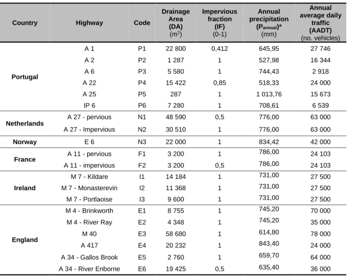
The assessment of the models was made considering the comparison between the prediction and monitored data. The former is related to SMC of 20 roads in Europe. These data were collected from direct contacts to the road and research institutes dealing with road runoff. A summary of the main characteristics of the monitored roads is presented in Table 3.1.
Table 3.1 – Road characteristics
Country Highway Code
Drainage Area (DA) (m2) Impervious fraction (IF) (0-1) Annual precipitation (Pannual)* (mm) Annual average daily traffic (AADT) (no. vehicles) Portugal A 1 P1 22 800 0,412 645,95 27 746 A 2 P2 1 287 1 527,98 16 344 A 6 P3 5 580 1 744,43 2 918 A 22 P4 15 422 0,85 518,33 24 000 A 25 P5 287 1 1 013,76 15 673 IP 6 P6 7 280 1 708,61 6 539 Netherlands A 27 - pervious N1 48 590 0,5 776,00 63 000 A 27 - Impervious N2 30 510 1 776,00 63 000 Norway E 6 N3 22 000 1 834,42 42 000 France A 11 - pervious F1 3 200 1 786,00 24 103 A 11 - impervious F2 3 200 0,5 786,00 24 103 Ireland M 7 - Kildare I1 14 184 1 731,00 27 500 M 7 - Monasterevin I2 11 368 1 731,00 27 500 M 7 - Portlaoise I3 9 600 1 731,00 27 500 England M 4 - Brinkworth E1 8 755 1 745,20 70 000 M 4 - River Ray E2 4 348 1 745,20 35 000 M 40 E3 58 680 1 614,80 78 000 A 417 E4 20 232 1 843,40 24 000 A 34 - Gallos Brook E5 2 760 1 659,70 64 000 A 34 - River Enborne E6 19 425 0,5 635,40 36 000
*Pannual information is available at: https://snirh.apambiente.pt/; https://www.climatedata.eu; https://fr.climate-data.org;
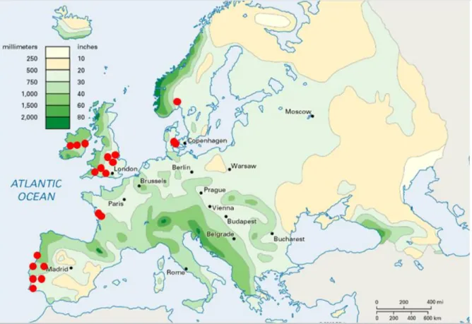
13 In Figure 3.1 the location of the monitored sites in an annual average precipitation map is presented.
Figure 3.1 – Europe precipitation map with the roads under study2. Each dot corresponds to one
road
As previously referred, in order to check which of the tools under study is better adapted to the collected data, the results predicted for each tool were compared to the monitored data. The monitored data is presented in Appendix 1. In order to treat the monitored data, for each site and each pollutant, the EMC values were averaged to calculate the mean SMC. These data were compared with the wastewater emission limit defined by the Portuguese Decree-Law n.º 236/98, from 01 of August. This analysis is presented in Table 3.2, where it was verified that only TSS are above the limit (60 mg/L). The precipitation hourly data series was collected or made available by the project partners.
Table 3.2 – SMC of each site
Highways (mg/L) TSS (µg/L) Cu (µg/L) Zn (µg/L) Pb (µg/L) Cd P1 22,96 19,24 124,07 4,38 0,09 P2 2,50 11,13 69,00 2,10 P3 19,65 8,10 345,83 1,83 P4 52,44 24,44 23,33 P5 57,93 86,86 139,69 28,65 P6 207,08 31,45 73,17 7,67 1,09 N1 114,71 500,88 29,88 1,60 2 https://eldoradoweather.com/forecast/climate/climate-maps/europe-annual-precip-map.html
14 Highways (mg/L) TSS (µg/L) Cu (µg/L) Zn (µg/L) Pb (µg/L) Cd N2 29,14 118,86 14,43 1,00 N3 227,61 84,09 224,87 14,70 0,21 F1 71,38 45,51 356,08 57,93 1,03 F2 10,89 27,37 160,05 11,64 0,43 I1 856,44 123,29 666,67 139,38 8,70 I2 155,74 48,95 198,25 68,91 4,86 I3 49,52 24,70 82,00 76,90 8,61 E1 88,60 30,00 100,70 E2 310,87 54,61 221,50 68,98 1,77 E3 50,88 42,65 149,31 15,16 0,43 E4 64,76 23,99 52,60 4,38 0,21 E5 101,13 67,92 219,73 50,45 0,62 E6 82,70 32,46 29,01 16,57 0,25 Decree-Law n.º 236/98 emission limit 60,00 1 000,00 1 000,00 200,00
3.2
Description of the models
PREQUALE
In the scope of the research project – G -Terra – funded by the Portuguese Foundation for Science and Technology and coordinated by the National Laboratory for Civil Engineering, the road runoff from several roads was monitored between 2002 and 2006 (Barbosa et al., 2011). Using the data of six roads, the first version of the tool PREQUALE which stands for Previsão da Qualidade das Águas de Escorrências (Road Runoff Quality Prediction) was developed. This tool aims at directly predict SMC. It is based on the following principles: (i) input data easily available for designers; (ii) easiness of calculation; (iii) clear and transparent model and (iv) reliable results at national level.
The applicability of the tool is rather simple as it is based on a multiparametric equation (equation 3.1) with the following input variables:
(i) Drainage area (DA in km2) – area which contributes with runoff to the discharge point during
a rainfall event;
(ii) Impervious fraction (IF in %) – the percentage of the total drainage area which is impervious; (iii) Average annual rainfall volume with the same duration as the basin time of concentration
(AR in mm) – further details on its calculation will be provided below; (iv) Annual average precipitation (Pannual in mm).
The multiparametric equation takes the following form:
15 where SMC is the estimated site mean concentration of each pollutant and ai, β1, β2, β3 and β4 are
the correspondingregression coefficients.
The AR was calculated in order to denote a representative rainfall event of the region. It was assumed that this event is the average precipitation with a duration equal to the time of concentration of the basin and with a return period of two years. To calculate this variable, it is necessary to use auxiliary calculations: firstly, the time of concentration of the drainage basin has to be determined (e.g. equation 3.2, in Lencastre and Franco, 1984).
tc= 0,0663 ×
DL1,155
Δh0,385 (3.2)
tc – Concentration time (hours)
DL – “Main river” length (Km) - (in this case is the maximum length of the road in the drainage basin) Δh – Slope (m) - heights difference between the ends of the road
Secondly, the volume is calculated using intensity-duration-frequency (IDF) curves with a return period of 2 years. For Portugal, the report Brandão et al. (2001) was used.
The current version of PREQUALE allows the prediction of SMC for TSS, chemical oxygen demand (COD), Fe, Zn and Cu. This tool was validated for the situations in which the parameters’ values were between the values presented in Table 3.3.
Table 3.3 – Intervals for which PREQUALE had been validated (Adapted from: Barbosa et al., 2011)
Parameter Lower limit Upper limit
AR (mm) 6,0 7,5
DA (Km2) 2,5×10⁻⁴ 6,5×10⁻²
IF (%) 40 100
Pannual (mm) 560 1 200
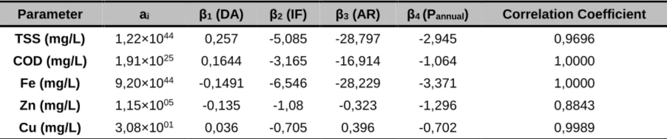
In Table 3.4 the road characteristics for each road used to calibrate PREQUALE are presented while the regression and correlation coefficients that resulted from the adjusted multiparametric equation of the roads SMC are presented in Table 3.5.
Table 3.4 – PREQUALE roads (Adapted from: Barbosa et al., 2011)
Road AR (mm) DA (km2) IF (%) P
annual (mm) Observations
A1 7,5 6,46×10⁻² 41,2 1 157,0 Runoff drains to the
treatment system
A3 Santo Tirso 6,8 2,00×10⁻³ 100,0 782,0 Descending section
A3 Ponte de Lima 6,1 2,45×10⁻³ 100,0 1 537,4 Ascending section
A6 6,5 5,58×10⁻³ 100,0 761,0 Runoff drains to the
treatment system
A25 6,0 2,50×10⁻⁴ 100,0 929,0 Near Aveiro lagoon
IP6 6,0 7,28×10⁻³ 100,0 902,0 Runoff drains to the
16 Table 3.5 – PREQUALE regression and correlation coefficients (Adapted from: Barbosa et al., 2011)
Parameter ai β1 (DA) β2 (IF) β3 (AR) β4 (Pannual) Correlation Coefficient
TSS (mg/L) 1,22×1044 0,257 -5,085 -28,797 -2,945 0,9696
COD (mg/L) 1,91×1025 0,1644 -3,165 -16,914 -1,064 1,0000
Fe (mg/L) 9,20×1044 -0,1491 -6,546 -28,229 -3,371 1,0000
Zn (mg/L) 1,15×1005 -0,135 -1,08 -0,323 -1,296 0,8843
Cu (mg/L) 3,08×1001 0,036 -0,705 0,396 -0,702 0,9989
Highways Agency Water Risk Assessment Tool (HAWRAT)
HAWRAT was developed by Highways Agency from the United Kingdom as a standalone application aiming at helping highway designers decide if road runoff pollution mitigation measures are needed.
This tool allows the prediction of (i) soluble pollutants and (ii) sediment related, expressed as EMC for total copper, zinc, cadmium, pyrene, fluoranthene, anthracene, phenanthrene and total PAH. As the model predicts EMC, it is necessary to calculate several EMC (in a time frame) in order to predict the SMC.
Besides the prediction of runoff quality, HAWRAT also incorporates models to predict the impact of the runoff on receiving rivers and streams, as shown in Figure 3.2. HAWRAT comprises three steps: Step 1 concerns road runoff pollution prediction, Step 2 is related to the impacts in the receiving water bodies and Step 3 deals with the selection of mitigation measures. In the scope of the present work, the results of steps two and three were not analysed.
Figure 3.2 – HAWRAT methodological scheme (Jotte et al., 2017)
HAWRAT should not be used in certain cases, such as: (i) Urban Highways; (ii) Highways with traffic densities outside the range of 11 000 – 159 000 vehicles/day (it can be used for highways with traffic density less than 11 000 vehicles/day but the result may be overestimated) and (iii) Highways discharging to receiving watercourse that are tidal and/or saline (Highways Agency, 2009). The agency also emphasises that the tool can be applied in Wales, Scotland and Northern Ireland, although the basic data was generated in England, and recalls its limited ability to assess the impact on streams where the flow is intermittent or seasonal.
17 As described by the Highways Agency (2009)
,
in order to use the graphical interface, HAWRAT uses an auxiliary software that stochastically generates hourly rainfall series of the United Kingdom and calculates a main part of the mandatory inputs of the tool.However, the pollutants that were intended to be studied in this work were not available in the automatic tool. Instead, the equation that was the basis of HAWRAT was used to predict the runoff pollution. This equation (equation 3.3) is a multiple linear regression resulting from a study (Crabtree et al. (2008) and Dempsey and Song (2008)). Equation 3.3 allows the user to predict TSS, total copper, total zinc and total cadmium and has the following input variables:
(i) Pollutant constant (PC) - Fixed to each pollutant;
(ii) Climate region constant (CRC) – Also fixed to each pollutant;
(iii) Annual average daily traffic constant (AADTC) – Dependent of the number of cars per day; (iv) Month constant (MC) – Fixed and based on the month that the precipitation event occurs; (v) Maximum hourly precipitation (MHI in mm/h) – The highest value of hourly precipitation
registered in a precipitation event;
(vi) Antecedent dry period (ADP in hours) – Number of hours without precipitation since the last precipitation event.
log10 EMC = PC + CRC + AADTC + MC + γ1 × MHI + γ2 × ADP (3.3)
Where log10EMC is the event mean concentration of the studied pollutant and γ1 and γ2 are the
regression coefficients presented in Table 3.6.
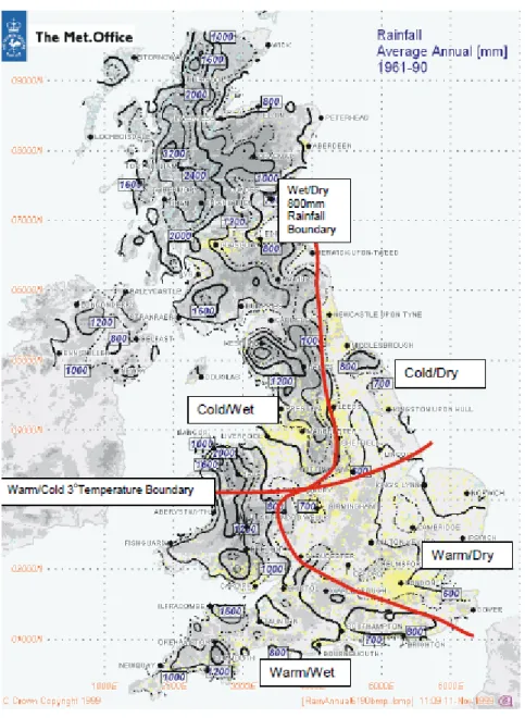
CRC is only defined for the region where HAWRAT is applicable (Figure 3.3). In this way, it was defined that the red lines that separate each climatic region will continue indefinitely, so the countries northwest of England will have an "cold/wet " climate, countries to the northeast will have a " cold/dry" climate, countries to the southwest will have a " warm/dry" climate and countries to the southeast will have a "warm/wet" climate.
18
Figure 3.3 – Representative map of the limits/areas used in HAWRAT (Crabtree et al., 2008)
The constants needed for the HAWRAT equation for each combination of region, traffic, month and pollutant are presented in Table 3.6.
Table 3.6 – Constants table in order to predict concentrations trough HAWRAT (Adapted from: Dempsey and Song, 2008)
Inputs EMC constants
Total Copper Total Zinc Total Cadmium TSS
S it e Constant 1,394 1,91 -0,832 2,1 Colder/Dry 0 0 0 0 Colder/Wet 0,042 0 0 -0,217 Warm/Dry 0,144 0 0 -0,248 Warm/Wet 0,089 0 0 -0,163
19
Inputs EMC constants
Total Copper Total Zinc Total Cadmium TSS
T raff ic AADT<50000 0 0 0 0 50000=<AADT<100000 0,018 0,045 0,093 0 AADT>=100000 0,512 0,502 0,379 0 Mon th s 1 0,402 0,662 0,773 0,535 2 0,568 0,699 0,565 0,443 3 0,526 0,704 0,625 0,324 4 0,427 0,504 0,374 0,193 5 0,559 0,716 0,579 0,288 6 0,425 0,32 0,241 0,283 7 0,258 0,27 0,064 -0,148 8 -0,064 -0,154 -0,216 -0,108 9 0,065 -0,098 -0,067 -0,101 10 0 0 0 0 11 -0,028 0,068 0,05 0,022 12 0,085 0,231 0,181 0,491 E xtra MHI 0 0,022 0 0,065 ADP 0 0 0 0
Kayhanian’s multiple linear regression method
Kayhanian et al. (2006) proposed a multiple linear regression (MLR) to predict EMC. This regression was undertaken with the following specific objectives: (i) Provide a statistically summary of highway runoff quality in California, United States of America (USA); (ii) Discuss the impact of selected independent event and site characteristics parameters on highway runoff constituent EMC and (iii) Evaluate the application of the MLR models as predictive tools to estimate the constituent EMC.
Stormwater runoff data used in Kayhanian et al. (2006) were obtained from 34 highway sites in California covering a wide range of annual average daily traffic levels and environmental conditions. These data were obtained, on average, up to eight storm events at each highway site during wet seasons (October to April) over a three years period (2000 to 2003). Some characteristics were recorded in each site, namely surrounding land use (obtained from United States Geological Survey maps, local zoning maps and visits to the sites), catchment area, impervious fraction, latitude and longitude and AADT.
Relationships were established by the authors between highway runoff quality for 24 constituents and the following independent variables:
(i) Total event rainfall (TER in mm) – height of rain of each precipitation event;
(ii) Antecedent dry period (ADP in days) – the number of days with no rain since the last precipitation event;
(iii) Cumulative seasonal rainfall (CSR in mm) – the total precipitation of a known season in a specific location.
20 (iv) Drainage area (DA in ha) – area which contributes with runoff to the discharge point during
a rainfall event;
(v) Annual average daily traffic (AADT in vehicles/day) – number of vehicles that pass each day in the location under study.
The adapted version of the general equation is presented below (equation 3.4). In Table 3.7, there are the constants used in the equation.
Ln EMC = β0+a × ln (TER) +b × ln (ADP) +c ×√CSR3 +d × ln (DA) +e×(AADT ×10-6) (3.4) Table 3.7 – Constants Kayhanian’s model (adapted from: Kayhanian et al., 2006)
Constituent β0 a b c d e Ag g regat es TSS 4,28 - 0,124 0,102 - 0,099 — 4,934 TDS 4,73 - 0,309 0,126 - 0,050 — 2,582 DOC 4,11 - 0,404 0,123 - 0,129 — — TOC 5,23 - 0,209 0,129 - 0,154 — — Me tals (t o tal) Cu 2,9 - 0,161 0,163 - 0,079 — 6,823 Pb 2,72 — — - 0,102 — 9,65 Ni 2,51 - 0,196 0,141 - 0,075 -0,155 1,013 Zn 4,83 - 0,227 0,143 - 0,084 — 6,747 Me tals (d iss o lve d ) Cu 2,92 - 0,290 0,185 - 0,102 — 3,679 Pb 2,04 - 0,248 — - 0,101 — 0,007 Ni 2,73 - 0,270 0,068 - 0,107 -0,094 — Zn 4,74 - 0,343 0,164 - 0,112 — 1,676 Nu tr ient s NO 3-N 1,3 - 0,417 0,092 - 0,090 — 2,87 P, total 1,2 - 0,143 0,128 - 0,051 — 0,9 TKN 1,7 - 0,343 0,102 - 0,128 — 1,535
* The table is not complete, missing the size of the samples used, the square root of the mean error and the standard error for each constituent. These data is available in Kayhanian et al., 2006.
Stochastic Empirical Loading and Dilution Model (SELDM)
SELDM was developed by the Federal Highway Administration from the USA and uses analytical approximations to estimate the potential effects of runoff on receiving waters. SELDM aims at predicting EMC, flows and loads in stormwater from a highway site and its upstream catchment. Using input information based on site characteristics, catchment characteristics, rainfall, stormflow, water quality and the performance of mitigation measures, this tool generates statistical distribution of runoff quality in highway runoff and receiving river water (Granato, 2013a).
SELDM uses a highway runoff database which contains data from over 4000 storm events, then uses the Monte Carlo method to generate the distribution of output variables such as EMC (Gardiner et al., 2016).
Novotny et al. (1993) as quoted by Santos and Barbosa in 2004 refers that the deterministic nature of most models to represent the variability of a phenomenon has originated some failures. In this case Monte Carlo method is used due to the combination of different variables (such as precipitation, pre-storm flows, runoff coefficients and water quality concentrations).
21 Granato and Jones (2014) described that SELDM uses Monte Carlo methods to generate a stochastic population of the concentrations, flows and loads needed to implement a mass balance model for a receiving stream and/or lake.
SELDM is not calibrated by changing values of input variables to match a historical record of values. Instead, SELDM’s input variables are based on site characteristics and representative statistics for each hydrological variable. The benefit of this method is not to reduce uncertainty in the input statistics, but to represent the different combinations of the values of variables that determine potential risks for water quality (Granato and Jones, 2014).
To estimate the concentrations and loads of water quality constituents in receiving bodies, a mass balance is commonly applied (Granato, 2013a) as shown in Figure 3.4.
Figure 3.4 – Mass balance for each storm event (Granato, 2013a)
Storm events are commonly defined as independent statistical events characterised by a volume, intensity, duration and time between midpoints of successive storms for the purposes of planning, analysis, and sampling efforts (Driscoll, 1990 in Granato, 2013a). Statistics describing the frequency distributions of component discharges and concentrations are needed to estimate the statistics for downstream discharges, concentrations, and loads (Granato and Jones, 2014).
The fact that SELDM was designed to predict road runoff pollution in US areas represents a limitation, which is common to every national based tool. In this case, the USA model defines “Ecoregions” where the parameters are already introduced. Nevertheless, the tool can be used in every region of the world with the manually input information of weather conditions.
The input layout of SELDM is a sequence of graphical user interface (GUI). In total 13 forms need to be completed with inputs information: (1) Information about the analyst, project and analysis; (2) Highway physical characteristics; (3) Ecoregion (when the site under study is in USA); (4) Upstream basin characteristics; (5) Lake basin characteristics; (6) Precipitation statistics (when the ecoregion is settled this form is almost automatically filled, however when the site is out of USA, it is necessary to calculate these data (see Table 3.8) outside the tool); (7) Streamflow; (8) Runoff coefficient statistics; (9) Highway runoff quality statistics; (9) Upstream water quality statistics; (10) Downstream water quality definitions; (11) BMP performance statistics; (12) Set of output files and (13) Running SELDM form. As for the road runoff pollution, only two of the 13 outputs are of interest, namely: (1) Precipitation event output file and (2) Highway runoff quality output file.
22 SELDM offers seven options for selecting storm-event statistics on the synoptic storm-event-precipitation statistics form as supported by the appendix 4 of SELDM help guide (Granato, 2013b). The default rain zone and ecoregion are automatically selected by entering the latitude and longitude of the highway site. The user, however, can manually select an ecoregion that better represents conditions at a site of interest. The option of entering user-defined statistics can be used to enter site-specific statistics, to do a sensitivity analysis, or evaluate the potential effects of climate change on model results (Granato, 2010). In this way, it is presented in Figure 3.5 the stochastically generated event rainfall volumes and in Figure 3.6 the same values but in an ordered series.
Figure 3.5 – Stochastically generated rainfall events with Portuguese data
Figure 3.6 – Ordered stochastically generated rainfall event for the same site in Portugal
In order to produce highway runoff quality output file, SELDM uses regional water-quality statistics to facilitate generation of initial planning-level estimates. If necessary, initial estimates can be refined with water-quality statistics based on available data collected at hydrologically similar sites or at the site of interest. SELDM also uses the Highway Runoff Database (HRDB) as source of highway runoff statistics and data, as stated by Granato and Cazenas (2009).
0 0,2 0,4 0,6 0,8 1 1,2 1,4 0 1000 2000 3000 4000 Rai n fa ll h e ig h t (i n )
Number of predicted events
0 0,2 0,4 0,6 0,8 1 1,2 1,4 0 1000 2000 3000 4000 Rai n fa ll h e ig h t (i n )
23 The HRDB application is designed as a data warehouse to document data and information from highway-runoff monitoring studies and as a pre-processor for highway-runoff data for use in SELDM. Available highway runoff data provide the basis for defining runoff quality and quantity at monitored sites and predicting runoff quality and quantity at unmonitored sites. HRDB includes data from 2 650 storms for 39 713 EMC measurements of more than 100 water quality constituents monitored at 103 sites in USA (Granato and Cazenas, 2009).
Inputs and outputs summary table
In the Table 3.8 are presented the inputs which are needed to run each model. Table 3.8 – Inputs summary table
Predicting tools
Inputs SMC EMC
PREQUALE HAWRAT Kayhanian's SELDM
Site characteristics CR X DA X X X IF X X AADT X X X AR X Pannual X X Others* Drainage Length (m); Mean Basin Slope (%)
Location (latitude and longitude); Drainage Length
(m); Mean Basin Slope; Basin Development factor
Event Characteristics Month X TER X X MHI X ADP X X X CSR X Others*
Average storm event durations; Minimum total
storm events; Minimum interevent time; Number of
storm events per year *As indicated above, SELDM is a tool which needs more inputs than physical and characteristics ones. So, beside those here presented in Table 3.8, SELDM needs the upstream basin characteristics, basin characteristics, streamflow statistics, runoff coefficients and best management practices (BMP) used in the road.
24 In the Table 3.9 is presented an outputs summary table.
Table 3.9 – Outputs summary table
Predicting tools
SMC EMC
PREQUALE HAWRAT Kayhanian's SELDM*
Aggregates TSS X X X X** TDS X DOC X TOC X COD X Metals (total) Cu X X X X Pb X X Ni X Zn X X X X Cd X X Fe X Metals (Dissolved) Cu X X Pb X Ni X Zn X X Nutrients (Total) NO-3 X X P X X KN X
* Besides these outputs, SELDM also has the following outputs: Urban TSS; Ultra Urban TSS; pH; suspended sediment concentration; Total chromium; Total Hardness
25
4
Assessment of the predicting tools
4.1
Methodology
Step 1
As presented in the previous section SELDM seems the most robust and complex model in terms of input requirements and output analysis. Since it did not result from a multi-parametric equation, a sensitivity test was carried out to verify if the methodology used in this section was adequate.
This dissertation aims to predict SMC starting only from hourly rainfall data of several meteorological stations. SELDM has its own “definition” of precipitation event fixing a minimum of 2,5 mm and an ADP of 6 hours (Granato, 2013a).
The inputs used in the sensitivity tests are presented in Table 4.1. These sensitivity tests were performed considering a reference test – Test 1, in appendix 4 of SELDM’s help guide (Granato, 2013b).
Table 4.1 – Sensitivity SELDM test inputs
SELDM Inputs Test
1 2 3 4 5 6 High w a y s it e : I de nti fy Site Cha rac te ris tic s Hydraulics Drainage area (acres) 18,50 3,70 1,85 0,93 92,50 185,00 Drainage length (feet) 2 000 400 200 100 10 000 20 000
Mean Basin slope
(feet per mile) 105,00 21,00 10,50 5,25 525,00 1 050,00
Impervious fraction (0-1) 0,27 0,05 0,03 0,01 0,60 0,80 Basin Development Factor (BDF) (0-12) 6 2 8 12 2 8 Sy no pti c St orm -Ev e n t p rec ipi ta tio n St a tis ti c s Storm-event statistics
Storm event volume
(inches) 0,68 0,14 0,07 0,03 3,40 6,80 Storm-event volume (COV) 1,06 0,21 0,11 0,05 5,30 10,60 Storm event duration (hours) 7,72 1,54 0,77 0,39 38,60 77,20 Storm event duration (COV) 0,90 0,18 0,09 0,05 4,50 9,00 Time between storm events (hours) 167,00 33,40 16,70 8,35 835,00 1 670,00 Time between
storm events (COV) 1,28 0,26 0,13 0,06 6,40 12,80
Minimum Total storm Volume (inches) 0,1 0,1 0,1 0,1 0,1 0,1 Minimum interevent time (hours) 6 6 6 6 6 6 Annual statistics and station count Number of storm
events per year 48,0 9,6 4,8 2,4 240,0 480,0
Number of storm events per year
(COV)
0,27 0,05 0,03 0,01 1,35 2,70
After running the tests, it was possible to determine the SMC for each test. The highway quality runoff output returns a series of storm events as explained in the section 3.2.4, and the pollutant EMC for each storm event. In Figure 4.1 is presented the results from the sensitivity tests.
26 Figure 4.1 – SMC of each test performed in the sensitivity test
Besides great variations in the input values for tests one to six, SELDM results of road runoff pollutant concentrations do not show great changes. This was an aid to the development of modeling with SELDM. Due to the high number of inputs required to run the program, and due to some difficulty in sometimes obtaining all these inputs from all project partners, it was possible to model some highways which were missing one or two input values, by using values that were consistent with the characteristics of the studied site.
Step 2
Since the average of the EMC of each event resulting from the output does not show great changes, a second approach to the same model was attempted. The case study of a Portuguese highway - A25 at Gafanha da Nazaré - which was previously monitored by Antunes (2014), was implemented in SELDM in order to compare monitored and predicted events. The model predicted 1346 events along with the precipitation characteristics of each event. The characteristics considered for the initial comparison between predicted (1346) and monitored (30) events were the rainfall volume, ADP and event-duration. From the 30 monitored events, 23 had at least one predicted event match, i.e. the values of the characteristics referred above were similar. On the other hand, there was no predicted event which matched the remaining seven monitored events. The second comparison was regarding the SMC. Like so, the 23 monitored events were compared with each matched predicted event and the results are present in Figure 4.2. Besides the fact that the deviation between monitored and predicted SMC values was not very large, it was noticed that the EMC values that were used to calculate the SMC, do not appear to have great similarity.
0,0 0,1 0,2 0,3 0,4 0,5 0,6 0,7 0 50 100 150 200 250
Test 1 Test 2 Test 3 Test 4 Test 5 Test 6
SM C fo r Cd SM C fo r T SS, Cu, Z n a n d Pb Performed Tests TSS (mg/L) Cu (µg/L) Zn (µg/L) Pb (µg/L) Cd (µg/L)