Abstract
Extruded aluminum profiles are widely used in building and au-tomation structures due to their durability, lightweight, corrosion resistance, shorter fastening time and reusability. Proper design is crucial in maintaining the lifespan of these structures. It is there-fore essential to determine the structural behaviors of the struc-tures such as the natural frequency, mode shape, etc. The finite element analysis is a method which has been commonly used in determining structural behaviors. However, there are also numer-ous problems in analyzing these kinds of profiles using solid finite elements, such as modeling, meshing, solution time problems, etc. Therefore, beam finite elements have been used in the present study in modeling of the profiles. Furthermore, an equivalent beam element model has been developed for bolt-together con-nectors of the profiles. Simulation and experimental modal analy-sis have been conducted on example test systems. It has been demonstrated that this modeling technique is very practical and the results obtained from the method agree well with the experi-mental results.
Keywords
Aluminum profile, aluminum structural framing, structures, finite element analysis, ANSYS.
Finite Element Analysis of Structures with Extruded
Aluminum Profiles Having Complex Cross Sections
1 INTRODUCTION
Modern engineering theories based on advanced engineering mathematics have been developed after the invention of the laws of motion. One of the major areas of modern engineering is the vibration theory. There are numerous studies in the literature on the vibration analysis of simple structures based on partial differential equations (Rao (2011)). The finite element (FE) method has been
de-Serkan Güler a Hira Karagülle b
a Department of Mechanical Engineering,
Faculty of Mechanics, İskenderun Tech-nical University, 31200, Hatay, Tur-key,[email protected]
b Department of Mechanical Engineering,
Engineering Faculty, Dokuz Eylül Uni-versity, 35397, İzmir,
Tur-key,[email protected]
http://dx.doi.org/10.1590/1679-78252755
veloped for modeling of realistic complex engineering systems. This method requires meshing of complex structures to finite elements and constructing mathematical models consisting of a set of differential equations with a large number of degrees of freedom. It has been possible to solve these equations after the development of digital computers. In the past, the analyzers constructed these equations and solved them by writing computer codes themselves. Further developments on com-puter softwares have made it possible to construct and solve the equations automatically. These user-friendly programs have pre-processors, solvers and post-processors (ANSYS (2009)). The users define the system under the study and make assumptions such as the types of finite elements, mesh sizes, etc. using the pre-processor. Then, they select the solution method and obtain the solutions. Finally, they evaluate the results using the post-processor. In recent years, one of the main research areas in engineering has been to develop realistic system models using these computer programs by appropriate assumptions (Akdağ et al. (2012), Zaeh et al. (2007), Wu (2004), Zaeh et al. (2004)). The accuracy of these assumptions could in turn be validated by comparing simulation results with experimental results.
Before the information age, simple structures were analyzed quantitatively and experience was very important for the analysis of complex structures. However, today, once the assumptions for the simulations are verified by experiments, complex structures can be analyzed quantitatively using validated simulation models. Thus, the importance of experience has lessened. This has enabled the researchers to develop solutions for complex engineering problems very rapidly.
Aluminum structural framing systems are widely used in industry. Aluminum profiles which have complex cross sections are preferred because they are durable, lightweight, corrosion resistant, reusable and readily available. These profiles are used in automation systems, conveyor frames, automobile body, work tables, interior design, and construction. Fewer tools and assembly time are required for assembling the system. The design is simple, and no welding and painting is required (Mazzolani (1995), Kwon et al. (2001), Mazzolani (2006)).
There are many studies which have investigated the structures that contain structural elements having simple cross sections such as square section, circular section, and rectangular section etc. (Wu (2006), Wu (2008), Hana et al. (2008), Sangle et al. (2012), Fadden et al. (2014)). On the oth-er hand, although the aluminum structural framing systems are extensively used in industrial appli-cations, there are limited investigations conducted for these profiles systems and their connection parts (Fiorino et al. (2013), Güler (2013), Macillo et al. (2013), Fiorino et al. (2014)). This is the motivation for the conduction of the current study.
2 STRUCTURES WITH ALUMINUM PROFILES
The frame of a test system (Frame-TS-1A) is shown in Fig 1. The labels for a beam (b01) and a connector (c01) are shown in the figure. The cross sections of the aluminum profiles and the con-necting parts used in the frames studied in this work are shown in Tables 1 and 2. All the parts used are available in the market.
(a) (b)
Figure 1: Solid model of frame of test system (a), photo of TS-1A (b).
Section Size (mm) File name Weight
(kg/m)
Area (cm2)
Moment of inertia
Ix (cm4) Iy (cm4)
90x90 s90x90 10.5 39.5 302 302
90x90 s90x90L 6.3 23.6 210 210
45x45 s45x45L 1.5 5.7 11 11
90x45 s90x45L 3.1 11.2 23.6 81.9
30x30 s30x30 0.8 3.1 2.7 2.7
Table 1: Cross sections of the profiles (Bosch Rexroth AG. (2013)).
Connector Weight(gr) Size (mm) File name
314a+187b 90x90x90 cn90
56a+47b 45x45x45 cn45
20a+17b 30x30x30 cn30
aWeight of connector, bWeigth of bolts and nuts
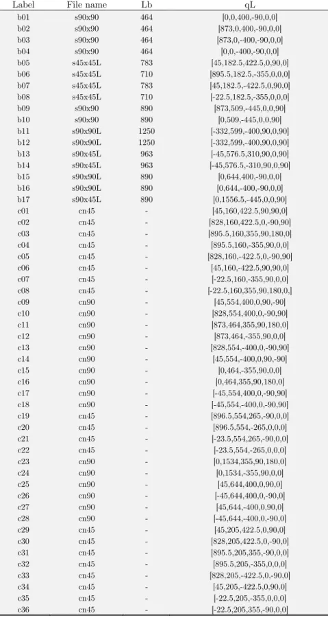
Label File name Lb qL
b01 s90x90 464 [0,0,400,-90,0,0] b02 s90x90 464 [873,0,400,-90,0,0] b03 s90x90 464 [873,0,-400,-90,0,0] b04 s90x90 464 [0,0,-400,-90,0,0] b05 s45x45L 783 [45,182.5,422.5,0,90,0] b06 s45x45L 710 [895.5,182.5,-355,0,0,0] b07 s45x45L 783 [45,182.5,-422.5,0,90,0] b08 s45x45L 710 [-22.5,182.5,-355,0,0,0] b09 s90x90 890 [873,509,-445,0,0,90] b10 s90x90 890 [0,509,-445,0,0,90] b11 s90x90L 1250 [-332,599,-400,90,0,90] b12 s90x90L 1250 [-332,599,-400,90,0,90] b13 s90x45L 963 [-45,576.5,310,90,0,90] b14 s90x45L 963 [-45,576.5,-310,90,0,90] b15 s90x90L 890 [0,644,400,-90,0,0] b16 s90x90L 890 [0,644,-400,-90,0,0] b17 s90x45L 890 [0,1556.5,-445,0,0,90] c01 cn45 - [45,160,422.5,90,90,0] c02 cn45 - [828,160,422.5,0,-90,90] c03 cn45 - [895.5,160,355,90,180,0] c04 cn45 - [895.5,160,-355,90,0,0] c05 cn45 - [828,160,-422.5,0,-90,90] c06 cn45 - [45,160,-422.5,90,90,0] c07 cn45 - [-22.5,160,-355,90,0,0] c08 cn45 - [-22.5,160,355,90,180,0,] c09 cn90 - [45,554,400,0,90,-90] c10 cn90 - [828,554,400,0,-90,90] c11 cn90 - [873,464,355,90,180,0] c12 cn90 - [873,464,-355,90,0,0] c13 cn90 - [828,554,-400,0,-90,90] c14 cn90 - [45,554,-400,0,90,-90] c15 cn90 - [0,464,-355,90,0,0] c16 cn90 - [0,464,355,90,180,0] c17 cn90 - [-45,554,400,0,-90,90] c18 cn90 - [-45,554,-400,0,-90,90] c19 cn45 - [896.5,554,265,-90,0,0] c20 cn45 - [896.5,554,-265,0,0,0] c21 cn45 - [-23.5,554,265,-90,0,0] c22 cn45 - [-23.5,554,-265,0,0,0] c23 cn90 - [0,1534,355,90,180,0] c24 cn90 - [0,1534,-355,90,0,0] c25 cn90 - [45,644,400,0,90,0] c26 cn90 - [-45,644,400,0,-90,0] c27 cn90 - [45,644,-400,0,90,0] c28 cn90 - [-45,644,-400,0,-90,0] c29 cn45 - [45,205,422.5,0,90,0] c30 cn45 - [828,205,422.5,0,-90,0] c31 cn45 - [895.5,205,355,-90,0,0] c32 cn45 - [895.5,205,-355,0,0,0] c33 cn45 - [828,205,-422.5,0,-90,0] c34 cn45 - [45,205,-422.5,0,90,0] c35 cn45 - [-22.5,205,-355,0,0,0] c36 cn45 - [-22.5,205,355,-90,0,0]
A database was created in a text file containing the information about the structure of the frame. The information about a beam is given by the label, the section file name, Lb, and qL = [x0, y0, z0, θx, θy, θz]. Lb is the length of the beam while qL is the location of the beam. x0, y0, and z0 are the Cartesian coordinates of the local origin of the beam in the global coordinate system. θx, θy,
θz are the rotation angles of the beam about the local x, y, and z axes, respectively. The beam is located at the origin and it is oriented in the global z axis for qL = qL0 = [0, 0, 0, 0, 0, 0]. The dis-tances are given in mm, and the angles are given in degree, unless otherwise stated.
The information about a connector is given by the label, the solid model file name, and qL. qL is the location of the connector. The labels start with the characters b and c for the beams and con-nectors, respectively. The database for the frame in Figure 1 is given in Table 3.
3 FINITE ELEMENT MODELS
3.1 Modeling with Solid Finite Elements
The easiest way of FE analysis after constructing solid model of the system is by using solid finite elements. ANSYS can use SolidWorks models, consider contacting surfaces, and perform meshing to generate solid finite elements. The user defines the boundary conditions and obtains the solution.
The disadvantages of this approach for complex systems are that the resulting number of ele-ments and degrees of freedom may be too large, meshing problems may arise, solution times may be too long, high performance computers may be required solutions may not be obtained, and analysis may not be practical.
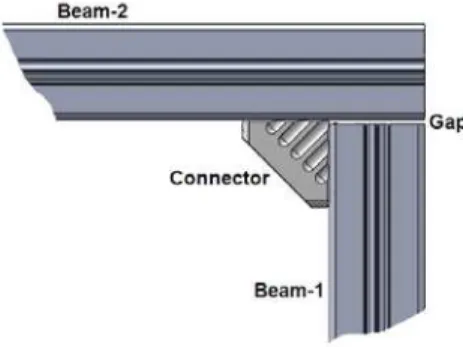
Small gaps (1 mm) between connected beams are given in the solid model as shown in Figure 2 for FE analyses. The gaps are given as decreasing lengths of beams. In this assumption, connected beam faces are mated to connector faces only and there is no direct contact between beams. The results are presented below for the models with gaps.
Figure 2: Gap given between connected beams
and β is the stiffness matrix multiplier for damping. Material properties are pm=[69,2700,0.3,0] for aluminum in this study.
3.2 Modeling with Beam Elements
Due to the disadvantages of the solid FE modeling as described above, the beam finite elements are used. In this approach, firstly, the lines are assigned for beams. The section attributes are defined for the lines. Two beams with a connector are shown in Figure 3 (a). The lines for the beam FE model are shown in Figure 3 (b).
(a) (b)
Figure 3:(a) Solid model, (b) Line model
Beam-1 and Beam-2 are created by the extrusions of corresponding cross-sections along the lines OA, and BC respectively. The extension beams are assumed on the lines E1E3 and E2E4. An equiva-lent beam for the connector is assumed on the line E1E2. E1 and E2 are at the mid-points of mating faces of the connector. The cross section of an extension beam is assumed to be the same as the adjacent beam. For example, E1E3 extension beam is assumed to have the same cross section as OA-beam. A negligible value (1 kg/m3) is assigned to the densities (ρ) of extension beams.
The properties of the cross sections of the equivalent beams of connectors are assigned by ana-lyzing L-frames as shown in Figure 3. Finite element analysis results are obtained by using solid finite elements and beam finite elements. The structure is fixed at O. Natural frequencies for the first two modes and the end point deflections at B under static loads are compared. The cross sec-tion properties of the connector are found by iterasec-tion so that the solid finite element results match with the beam finite element results. The value of ρ for an equivalent connector beam is assigned so that the equivalent connector beam has the same mass as the real connector.
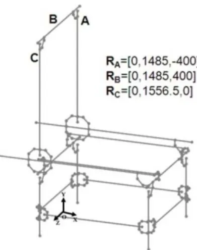
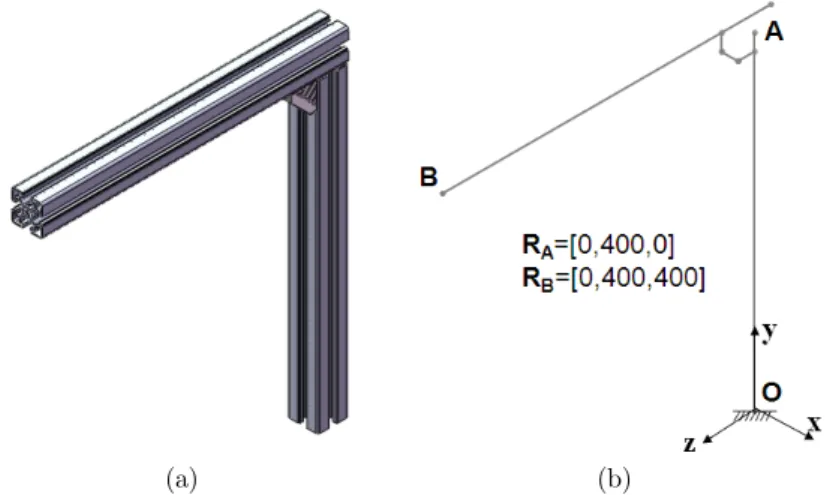
The lines for the beam FE model of Frame-TS-1A are shown in Figure 4. The location of a point (Point-A) on the line model of a system is defined by RA = [xA, yA, zA], where xA, yA, and zA are global Cartesian coordinates. O is the global origin. The locations of the points which are used for the results below are given in the figure. These points are used as excitation or sensor points below.
Figure 4: Line model of Frame-TS-1A
BEAM44 elements are used in ANSYS for beams. BEAM44 is a uniaxial element with tension, compression, torsion, and bending capabilities. The element has 6 degrees of freedom at each node: translations in the nodal x, y, and z directions and rotations about the nodal x, y, and z-axes. This element allows a different unsymmetrical geometry at each end and permits the end nodes to be offset from the centroidal axis of the beam. The details of the element are given in theory reference of ANSYS (ANSYS (2009)). Let a beam element has the nodes at the points I and J. The cross section of an element at I is shown in Figure 5, schematically.
Figure 5: Cross section of beam element at Node-I
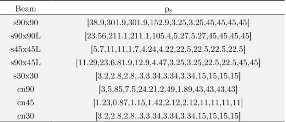
w.r.t. the axis in the z direction passing through G. IGz equals to the polar moment of inertia if IGz=IGx+IGy . IGz=IGt, if IGz equals to the torsional moment of inertia. The units of area moment of inertias are taken as cm4 unless otherwise is stated. Sdx and Sdy are the shear deflection constants. T, B, L, R are the points on the fibers at extreme distances from G. xG and yG are the nodal coor-dinates of G. qG= [0, 0] if there is no offset between the nodal origin and the area center of gravity of the cross section. It is assumed that there is no offset unless it is stated. The geometrical proper-ties of the beams are given in Table 4. The cross-sectional properproper-ties of beams are found by import-ing cross-section files to ANSYS.
Beam ps
s90x90 [38.9,301.9,301.9,152.9,3.25,3.25,45,45,45,45] s90x90L [23.56,211.1,211.1,105.4,5.27,5.27,45,45,45,45] s45x45L [5.7,11,11,1.7,4.24,4.22,22.5,22.5,22.5,22.5] s90x45L [11.29,23.6,81.9,12.9,4.47,3.25,3.25,22.5,22.5,45,45]
s30x30 [3.2,2.8,2.8,.3,3.34,3.34,3.34,15,15,15,15] cn90 [3,5.85,7.5,24.21,2.49,1.89,43,43,43,43] cn45 [1.23,0.87,1.15,1.42,2.12,2.12,11,11,11,11] cn30 [3.2,2.8,2.8,.3,3.34,3.34,3.34,15,15,15,15]
Table 4:Geometrical properties of beams
4 MODELING SOFTWARE
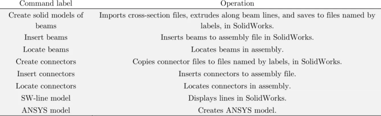
A computer program to create SolidWorks and ANSYS models of aluminum profile framing (APF) systems has been developed in VisualBASIC. The users can create a database file for APF systems. The database contains the following information for FE analysis of frames: the information about the beams and connectors as listed in Table 3; the information about the boundary conditions, the meshing size; the geometrical properties of cross sections, and the material properties. User interface of the developed computer program is shown in Figure 6. The list of the operations is given in Ta-ble 5. The execution of the operations is activated by clicking the corresponding command options. The operations are achieved by using the input database and Application Programming Interface (API) capabilities of SolidWorks.
Command label Operation Create solid models of
beams
Imports cross-section files, extrudes along beam lines, and saves to files named by labels, in SolidWorks.
Insert beams Inserts beams to assembly file in SolidWorks.
Locate beams Locates beams in assembly.
Create connectors Copies connector files to files named by labels, in SolidWorks.
Insert connectors Inserts connectors to assembly file.
Locate connectors Locates connectors in assembly.
SW-line model Displays lines in SolidWorks.
ANSYS model Creates ANSYS model.
Table 5: List of operations of modeling software
5 MEASUREMENT SYSTEM
The measurement system for obtaining experimental results is shown in Figure 7. The wireless vi-bration sensor is a MicroStrain G-Link tri-axial accelerometer (Accelerometer range: ± 10 g, 47 g, 58 mm x 43 mm x 26 mm). The wireless base station is MicroStrain Gateway WSDA-Base-104. The data received by the base station is transmitted to the computer through Universal Serial Bus (USB) and recorded by using Node Commander Software. The sampling rate is 2048 Hz. The frame is excited by a hammer impact. The FFTs (Fast Fourier Transforms) of the recorded signals in the x, y, and z directions are taken in MatLAB. The frequencies where the peaks appear are determined for the natural frequencies.
Figure 7: Photos of measurement system.
6 RESULTS AND DISCUSSIONS
6.1 L-Frame (LF-45)
(a) (b)
Figure 8: L-frame (LF-45) (a) Solid model for simulations (b) line model.
Label File name Lb qL
b01 s45x45 450 [0,0,0,-90,0,0]
b02 s45x45 450 [0,472.5,-22.5,-0,0,0]
c01 cn45 - [0,450,22.5,90,0,0]
Table 6: Database for L-frame (LF-45)
The properties of the computers used to obtain FE results are given in Table 7. The solution time (s) for Type-1 computer is t1, the solution time (s) for Type-2 computer is t2, the number of nodes for FE analysis is nd, and these values are given by sp=[t1,t2,nd].
Computer Properties
Type-1 WORKSTATION Intel Xeon X5687 3.6 GHz, 24 GB RAM, 64 Bit Win7 Operating System
Type-2 AMD PHENOM II X4 955- 3.2 GHz, 8GB RAM, 64 Bit Win7 Operating System
Table 7: Properties of computers
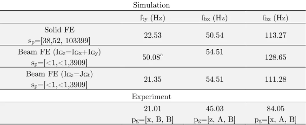
Simulation
fty (Hz) fbx (Hz) fbz (Hz)
Solid FE
sp=[38,52, 103399] 22.53 50.54 113.27
Beam FE (IGz=IGx+IGy)
sp=[<1,<1,3909] 50.08
a 54.51 128.65
Beam FE (IGz=JGt)
sp=[<1,<1,3909] 21.35 54.51 111.28
Experiment 21.01 pg=[x, B, B]
45.03 pg=[z, A, B]
84.05 pg=[x, A, B]
a Mode shape is different than torsional vibration about the y-axis
Table 8: Natural frequencies for LF-45
(a) (b) (c)
Figure 9: Mode shapes of LF-45 with solid finite elements for LF-45, (a) Mode-ty, (b) Mode-bx, (c) Mode-bz.
0 0.5 1 1.5 2
−30 −20 −10 0 10 20 30 Time Data Time (s) ax (m/s 2)
0 0.5 1 1.5 2
−20 −10 0 10 20 Time Data Time (s) ay (m/s 2)
0 0.5 1 1.5 2
−20 −10 0 10 20 Time Data Time (s) az (m/s 2)
0 5 10 15 21.01 25 30 35 40
0 2 4 6 8 Frquency (Hz) FFT of Axis X Acceleration Data
0 10 35 45.03 55 70 80
0 2 4 6
Frquency (Hz) FFT of Axis Y Acceleration Data
0 21.01 45.03 84.05 150
0 0.5 1 1.5
Frquency (Hz) FFT of Axis Z Acceleration Data
(a) (b) (c)
Figure 10: FFT’s of signal components and acceleration signal for experimental results in
The excitation point and direction and the sensor axis (component) are chosen so that mainly the mode of interest is excited. The maximum values of the amplitudes of FFT’s give the experi-mental natural frequencies. It is observed from Table 8 that the simulation result for Mode-ty is highly different than the experimental result if the polar moment of inertia were used. The use of torsional moment of inertia is important to obtain matching simulation and experimental results. The experimental values are smaller than the simulation results.
6.1 Frames (TS-1)
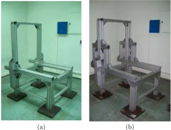
The results are given for Frame TS-1A, Frame TS-1B, and Frame TS-1C in this section. The database for Frame TS-1A shown in Figure 1 is given in Table 3. Frame TS-1B is obtained by rein-forcing Frame TS-1A. Frame TS-1C is obtained by reinrein-forcing TS-1B. Added components are given in Tables 9 and 10. Reinforcing is carried out by considering the mode shapes. The photos of Frame TS-1B and Frame TS-1C are shown in Figure 11.
(a) (b)
Figure 11: Photos of (a) Frame TS-1B, and (b) Frame TS-1C
Label File name Lb qL
bt01 s90x90L L [0,h,490,-90,0,0]
bt02 s90x90L L [0,h,-490,-90,0,0]
ct01 cn90 - [0,h,445,90,0,0]
ct02 cn90 - [0,h+L,445,0,0,0]
ct03 cn90 - [0,h,-445,180,0,0]
ct04 cn90 - [0,h+L,-445,-90,0,0]
ct05 cn90 - [45,599,445,0,0,-90]
ct06 cn90 - [-45,599,445,0,0,90]
ct07 cn90 - [45,599,-445,-90,0,-90]
ct08 cn90 - [-45,599,-445,-90,0,90]
ah is changed. L=530, h=240 unless otherwise stated
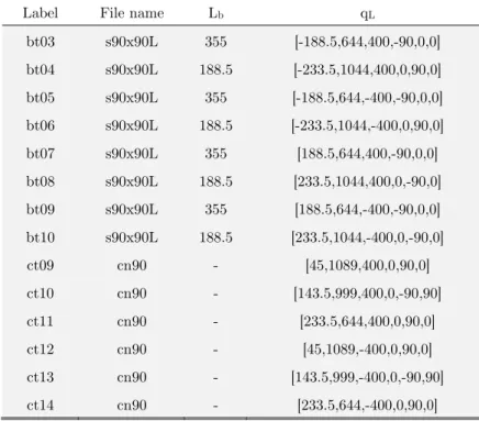
Label File name Lb qL
bt03 s90x90L 355 [-188.5,644,400,-90,0,0]
bt04 s90x90L 188.5 [-233.5,1044,400,0,90,0]
bt05 s90x90L 355 [-188.5,644,-400,-90,0,0]
bt06 s90x90L 188.5 [-233.5,1044,-400,0,90,0]
bt07 s90x90L 355 [188.5,644,400,-90,0,0]
bt08 s90x90L 188.5 [233.5,1044,400,0,-90,0]
bt09 s90x90L 355 [188.5,644,-400,-90,0,0]
bt10 s90x90L 188.5 [233.5,1044,-400,0,-90,0]
ct09 cn90 - [45,1089,400,0,90,0]
ct10 cn90 - [143.5,999,400,0,-90,90]
ct11 cn90 - [233.5,644,400,0,90,0]
ct12 cn90 - [45,1089,-400,0,90,0]
ct13 cn90 - [143.5,999,-400,0,-90,90]
ct14 cn90 - [233.5,644,-400,0,90,0]
Table 10: Added component to TS-1B for TS-1C.
The results are given in Tables 11, 12, and 13 for Frame TS-1A, TS-1B, and TS-1C, respective-ly. The mode shapes obtained from simulation of TS-1 B are depicted in Figure 12. See Figure 4 for the locations of the excitation and the sensor points.
(a) (b) (c)
Figure 12: Mode shapes of Frame TS-1B, (a) Mode-bx, (b) Mode-ty, (c) Mode-bz
fbx (Mode-bx) fbz (Mode-bz) fty (Mode-ty)
Simulation Beam FE (IGz=JGt)
sp=[15,19,149317] 31.52 40.34 58.06
Experiment 30.74
pg=[z, A, C]
39.42 pg=[x, B, C]
56.35 pg=[x, A, C]
Table 11: Natural frequencies for Frame TS-1A
fbx (Mode-bx) fbz (Mode-bz) fty (Mode-ty)
Simulation Beam FE(IGz=JGt)
sp=[16,23,166911] 43.72 42.88 61.22
Experiment 38.91
pg=[z, A, C]
41.98 pg=[x, B, C]
61.46 pg=[x, A, C]
Table 12: Natural frequencies for Frame TS-1B
fbx (Mode-bx) fbz
(Mode-bz) fty (Mode-ty)
Simulation Beam FE(IGz=JGt)
sp=[19,27,199059] 36.83 50.62 61.25
Experiment 33.29
pg=[z, A, C]
43.53 pg=[x, B, C]
58.89 pg=[x, A, C]
Table 13: Natural frequencies for Frame TS-1C
The experimental results given in Table 11 show that Mode-bx, Mode-bz, and Mode-ty have natural frequencies of 30.74, 39.42, and 56.35 Hz. These frequencies increase by 8.17, 2.56, and 5.11 Hz, respectively, for TS-1B as observed in Table 12. These frequencies increase by 2.55, 4.11, and 2.54 Hz, respectively, for TS-1C as observed in Table 13.
The simulation and experimental results show similar trend for increasing natural frequencies with reinforcement. Reinforcing in TS-1B is more effective to increase the natural frequencies. Nat-ural frequencies increase as stiffness/mass ratio effect of reinforcing increase.
7 CONCLUSIONS
Assumptions were made to model connectors with beams. Simulation and experimental results were given for different frames. The results show that the approach developed in the present article can be used to design frames with aluminum profiles, which are commonly used in many engineer-ing applications.
Acknowledgements
The authors would like to acknowledge Turkish Scientific and Research Council (Project number: 110M131) for its financial support of this work.
References
Akdağ, M., Karagülle, H. and Malgaca, L. (2012). An integrated approach for simulation of mechatronic systems applied to a hexapod robot. Mathematics and Computers in Simulation, 82:818-835
Bosch Rexroth AG.(2013.) Basic Mechanical Elements, 3 842 540 392.
Fadden, M. and McCormick, J.(2014). Finite element model of the cyclic bending behavior of hollow structural sec-tions. Journal of Constructional Steel Research. 94: 64–75.
Fiorino, L., Macillo, V. and Mazzolani, FM .(2014) Mechanical behaviour of bolt-channel joining technology for aluminium structures. Construction and Building Materials 73: 76–88.
Fiorino, L., Macillo, V., Mazzolani, FM.(2013). Screwed joint for aluminium extrusions: experimental and numerical investigation. In:12th INALCO conference, Montreal 21–22 October 159–169.
Güler, S.(2013) Finite element analysis of a vertical machining center with aluminum profile framing. PhD Thesis, Dokuz Eylül University, İzmir, Turkey.
Hana, LH.,Wanga, WD., Zhao, XL.(2008). Behaviour of steel beam to concrete-filled SHS column frames: Finite element model and verifications. Engineering Structures 30, (6):1647–1658.
http://www1.ansys.com/customer/content/documentation/121/ans_thry.pdfs (2009) Accessed 10 March 2010 Kwon, HC., Im, YT., Ji, DC. and Rhee, M.H.(2001). The bending of an aluminium structural frame with a rubber pad. Journal of Materials Processing Technolog.113(1–3): 786–791.
Macillo, V., Fiorino, L. and Mazzolani, FM.(2013). Structural behavior of aluminium bolt channel joint: calibration of numerical models on testing results, In: 12th INALCO conference, 148-158, Montreal 21–22 October (2013). Mazzolani FM. (2006). Structural applications of aluminium in civil engineering. Structural Engineering Internation-al, International Association for Bridge and Structural Engineering. 16:280-285.
Mazzolani, FM.(1995). Aluminium Alloy Structures. 2nd ed. London: E & FN SPON.
Microsoft. Help for Visual Basic 6 Users. https://msdn.microsoft.com/en-us/library/kehz1dz1(v=vs.90).aspx. (2012) Accessed 27 April 2012.
Rao, SS.(2011). Mechanical Vibrations. 3rd ed. Upper Saddle River: Prentice Hall.
Sangle, KK., Bajoria, KM. and Talicotti, RS.(2012) Elastic stability analysis of cold-formed pallet rack structures with semi-rigid connections. Journal of Constructional Steel Research. 71, 245–262.
Solidworks Web Help, Solidworks Corporation, http://help.solidworks.com (2012). Accessed 27 April 2012 Theory Reference for the Mechanical APDL and Mechanical Applications, ANSYS Release12.1:
Wu, JJ.(2006). Finite element analysis and vibration testing of a three-dimensional crane structure. Measurement. 39 (8), 740–749.
Wu, JJ.(2008). Transverse and longitudinal vibrations of a frame structure due to a moving trolley and the hoisted object using moving finite element. International Journal of Mechanical Sciences. 50 (4): 613–625.
Zaeh, M. and Siedl, D.(2007) A new method for simulation of machining performance by integrating finite element and multi-body simulation for machine tools. Annals of the CIRP. 56: 383-386.