ISSN 0102-261X www.scielo.br/rbg
SEISMIC DATA INVERSION BY CROSS-HOLE TOMOGRAPHY
USING GEOMETRICALLY UNIFORM SPATIAL COVERAGE
Armando Luis Imhof
1, Carlos Adolfo Calvo
2and Juan Carlos Santamarina
3Recebido em 25 fevereiro, 2008 / Aceito em 18 abril, 2009 Received on February 25, 2008 / Accepted on April 18, 2009
ABSTRACT.One of the inversion schemes most employed in seismic tomography processing is least squares and derived algorithms, using as input data the vector of first arrivals. A division of the whole space between sources and receivers is performed, constructing a pixel model with its elements of the same size. Spatial coverage is defined, then, as the sum of traveled length by all rays through every pixel that conform the medium considered. It is related, therefore, with the source-receiver’s distribution and the form of the domain among them. In cross-hole array, rays do not evenly sample the properties of the medium, leading to non-uniform spatial coverage. It is known that this affects the inversion process. The purpose of this paper, then, was to study the problem of spatial coverage uniformity to obtain travel path matrices leading to inversion algorithms with better convergence. The medium was divided in elements of different size but with an even spatial coverage (named as ‘ipixels’), and then it was explored how this improved the inversion process. A theoretical model was implemented with added noise to emulate real data; and then the vector of measured times was generated with known velocity distribution. Afterwards an inversion method using minimum length solution was performed to test the two domain divisions. The results showed that the fact of using ipixels not only improved the inversion scheme used in all cases; but in addition allowed to get convergence where it was impossible to do using pixels; particularly through the method considered. This is a direct result of the improvement of condition number of the associated matrices.
Keywords: seismic tomography, cross-hole, spatial coverage, pixel, ipixel.
RESUMEN.Uno de los esquemas de inversi´on m´as empleados en el procesamiento de datos de tomograf´ıa s´ısmica es el de m´ınimos cuadrados y algoritmos relacionados, utilizando el vector de primeros arribos como datos de entrada. Se lleva a cabo una divisi´on del dominio completo entre emisores y receptores, con el objeto de dise˜nar un modelo de p´ıxeles del mismo tama˜no. Se define la cobertura espacial como la suma de los tiempos de viaje de todos los rayos en cada uno de los p´ıxeles que conforman el medio. Por lo tanto este par´ametro est´a relacionado con la distribuci´on emisor-receptor y con la forma del dominio entre los mismos. En el dispositivo cross-hole los rayos no muestrean de igual forma al medio, conduciendo a una cobertura espacial no uniforme. Se sabe que este inconveniente afecta el proceso de inversi´on. El prop´osito de este art´ıculo fu´e el de estudiar el problema de la uniformidad de la cobertura espacial a fin de lograr matrices de tiempo de viaje que conduzcan a algoritmos de inversi´on con mejor convergencia. El medio se dividi´o en elementos de diferente tama˜no pero con cobertura espacial uniforme (denominados ‘ipixels’). Se implement´o un modelo te´orico con ruido a fin de simular datos reales; y el vector de tiempos se calcul´o con una distribuci´on conocida de velocidades. Luego se prob´o la convergencia de las dos formas de divisi´on del dominio utilizando el m´etodo de soluci´on por m´ınima longitud del vector de tiempos. Los resultados demostraron que el hecho de emplear ipixels no solo mejor´o la inversi´on en todos los casos, sino adem´as permiti´o lograr convergencia en casos donde result´o imposible utilizando pixeles; particularmente con el m´etodo utilizado. Este es un resultado directo del aumento de la condici´on de las matrices asociadas.
Palabras-clave: tomograf´ıa s´ısmica, cross-hole, cobertura espacial, pixeles, ipixeles.
1Instituto Geof´ısico Sismol´ogico Volponi, Facultad de Ciencias Exactas F´ısicas y Naturales, Ignacio de la Roza y Meglioli. Rivadavia, C.P. 5400, San Juan, Rep´ublica Argentina. Phone: +54(264) 494-5015; Fax: +54(264) 423-4980 – E-mail: [email protected]
2 Departamento de Matem´atica, Facultad de Ingenier´ıa, Av. Libertador Gral. San Mart´ın, 1109 (O) C.P. 5400, San Juan, Rep´ublica Argentina – E-mail: [email protected] 3Center for Applied Geomaterials Research. Atlanta, Georgia. USA. http://geosystems.gatech.edu. Postal address: Instituto Geof´ısico Sismol´ogico Volponi, Ruta 12, Km 17, C.P. 5413, Rivadavia, San Juan, Rep´ublica Argentina – E-mail: [email protected]
INTRODUCTION
Cross-hole travel-time tomography surveys consist of registe-ring the first arrival pulses of waves that travel through subsur-face between seismic sources and receivers (e.g. geophones, hy-drophones) located at opposite sides between boreholes (Sheriff & Geldard, 1995) (Fig. 1).
Transducers: 7 sources (left) 7 receivers (right) 49 rays.
Figure 1 – Ray tracing. Discretization of space in 49 pixels. Cross-hole array. When attempting to model anomalies between boreholes in geophysical exploration, it is necessary to manage some kind of inversion scheme after the pre-processing tasks of the survey data, to be able to assess some kind of geophysical model about the medium involved. The tomographic result consists, generally, in a slowness or velocity distribution through the domain that permits to discover variations in it, which will lead to detect the anomalies sought, if any.
In this work the ray theory will be employed, considering both the host medium and the inclusion as homogeneous (with different velocities), rendering straight-ray propagation (Kolsky, 1963). This approximation is well suited for depths greater than 10m as was demonstrated by Imhof (2007). At smaller ones, stress-dependent anisotropy and heterogeneity are present producing ray bending, therefore eliminating the independence between the model raypath matrix and the parameters investi-gated, and so complicating the inversion (Santamarina & Reed, 1994; Santamarina et al., 2001).
After the acquisition and through the picking and pre-processing tasks, the vector of travel timesy<meas>is formed
withM ×1 length; being M number of measurements (i.e. equa-tions). The problem, then, lies to apply an inversion technique to solve the system:
y<meas>= S ∙ x<est> (1) whereS is the M × N raypath matrix that represents the mo-del and x<est> theN × 1 vector of unknown slownesses (or velocities) distribution.
Consideringx<est>, it is important to quote that generally
two forms of representation exist in order to face the inversion scheme:
a) Parametric based: the medium is considered withfew un-knowns: host velocityVhost(constant), inclusion velocity
Vinc(if any, constant too), parameters that locate it:xinc,
yinc; and finally other that permit to assess its form and
size, i.e. circular or elliptical (see Santamarina & Cesare, 1994; Imhof & Calvo, 2003; Imhof, 2007). This will lead to an over-determined system of equations that, when pos-sibly, is solved with variational or least squares inversion algorithms, for example.
b) Pixel based: The medium is divided in N uniform (i.e. same size) pixels; each of them is an unknown with a par-ticular estimated (after the inversion) velocity or slowness value. When the inversion process is finished, an image reconstruction will show the position of each element and its velocity value (or colour pattern related). This will show the position of inclusion through colour contrast (Taran-tola, 1987; Menke, 1989; Fernandez, 2000). It is clear that the smaller the pixels, the better the image resolution ob-tained, but at the cost ofN increment, leading so to an under-determined system of equations.
Though in (b) a uniform pixel representation was mentioned, other forms to divide the medium can be studied; since the usual form leads to uneven distribution in spatial coverage (see Theory). The primary objective of this paper is to implement a different form of discretization of the medium with the purpose to study first the conditioning and rank of several raypath matrices made with those distinct elements assembly; and second use them to study their behavior with a typical inversion method using a theoretical model constructed to that end.
THEORY
Forward and inverse problem
Keeping in mind straight ray theory, the forward problem per-mits to compute thepredicted (output) travel time vectory<pred>
(M ×1) as a function of the vector of known true slownesses (in-put)x<true>(N×1), and the transformation matrix S (M×N), which represents the travel path that connects ‘x’ to ‘y’;
y<pred>= S ∙ x<true> (2)
In the inverse problem, theM values collected in vector y are
parametersx<est>:
x<est>= S−1∙ y<meas> (3)
In general (as in this case) the inverseS−1cannot be
de-termined, and a pseudo inverse must be used instead (Penrose, 1955):
x<est>= S<pseudoinv>∙ y<meas> (4)
In a well posed problem the solution exists and is unique and stable (Santamarina & Fratta, 1998). The problem here is that cross-hole tomography is not a well posed problem because of the relative distribution of sources and receivers (Branham, 1990; Tarantola, 2005) that involves rays almost parallel which increase condition number of associatedS matrix.
The procedure is to calculate first the appropriate matrixS of travel paths, then evaluate its pseudoinverse S<pseudoinv>
(depending of the method of inversion considered) and last to apply Eq. (4) to findx<est>.
Considering straight path simplifies very much the formula-tion at hand because the matrixS must be assembled only once (explicit form).
Raypath matrix
The entries inS (Fig. 2) are calculated identifying the intersec-tion of the individual ‘m’ ray with the ‘n’ pixel boundaries and computing the Pythagorean length ‘d’ inside the element.
Therefore, the size ofS will grow with the increment of mea-surements and/or discretization density.
Considering again Figure 1 and having still in mind Figure 2; the number of sources and receivers there is 7 and so the total number of rays is 49 (constant for this array). If the medium is divided in 7×7=49 pixels, S will be of 49 rows (M, number of rays) per 49 columns (N, number of pixels, whose slownesses are unknown). It is relevant to note that the increment of the pixel density (N), will lead to consider more pixels in the computation of travel paths for each receiver.
This system of equations is apparently even-determined (equal number of equations than unknowns). The word apparen-tlymeans that in some cases (especially in cross-hole, see Imhof, 2007) the system is ill conditioned and the rank ofS < N, M. This will give an underdetermined system leading to infinite so-lutions. The same will occur, for example, dividing the medium in more pixels to improve the resolution of the images. (the limita-tion of dividing the medium withN = M is that the resolution is coarse, because the size of the pixels is large).
Incrementing the number of transducers to improve resolu-tion is not practical and always possible to do; first, due to the
amount of survey effort needed (cost) and, second, if rays are so near, the condition ofS matrix augment and not necessar-ily add information to the system (Santamarina & Fratta, 1998; Fernandez, 2000).
Matrix of Spatial coverage (Sc)
As quoted, the size ofS is M rows (number of measurements) perN columns (number of unknown pixel slownesses). The sum of each individual column ofS brings the total length traveled by the rays inone pixel (Fig. 2). Applying this summation in all co-lumns ofS, gives a 1 × N row vector that re-arranged following the geometric pattern, brings theSc matrix of ‘s’ vertical pixels by ‘t’ horizontal ones where N = s + t. It was considered here
s = t.
Two examples of cross-holeSc matrices are represented in Figure 3 for 10 source-receiver’ pairs; (a) for 100 elements and (b) 400 ones. The dark zones indicate lower values of spatial co-verage.This means that the information gathered to solve the ve-locity or slowness of it is lower than in other lighter zones. In other wordsthe precision for the evaluation of the pixel values will not be uniform. Due to more rays traversing one pixel get more infor-mation of it (similar to CDP concept in reflection seismics), the lightest sector at the center ofSc matrix depicts the maximum resolution and precision for the pixel/s situated there. But what happens when an inclusion being searched for is far from that po-sition? The resolution to locate it will be poorer (Santamarina & Fratta, 1998).
An alternative form to divide the medium to improve the re-solution in the dark zones is proposed: Instead of separate it in pixels of same size and different spatial coverage at each; it’ll be divided in elements of equal spatial coverage and distinct indivi-dual sizes and named as ipixels. Due to this fact, the elements of S will be different. Figure 4 shows the domain divided in two den-sities of ipixels. The same color tones depict same information at each element.
Any type of element discretization for the physical domain is perfectly possibly to accomplish, because any type of it is only geometrical and has for purpose to make theS matrix and arm the system of equations having the distances traveled by the rays.
Conditioning of a matrix
If there is a high contrast between numerical values of the ele-ments inside a matrix; it is possible that the calculated rank for it has an erroneous linearly independent number of rows. Due to this, the condition number κ is a better choice to study the
=
...
...
...
...
...
...
...
...
...
...
...
...
...
...
...
....
1 1 1 1 11∑
= = 1 : raypath matrix:length travelled by ray ‘m’ in pixel ‘n’ : length travelled by all rays in pixel ‘n’. : number of travel-time measurements
: number of pixels. pixel ‘n’ ray ‘m’ source receiver d Borehole Borehole
Figure 2 – Raypath matrix assembly and meaning of spatial coverage.
(a) (b)
Figure 3 – Spatial coverage graphs for pixels. (a) 10×10 pixels, (b) 20×20 pixels. conditioning of a matrix (i.e. how near it is of a matrix of lower
rank) than its rank (Strang, 1980).
κis defined as the ratio between the singular values with ma-ximum and minimum absolute values (Golub & Van Loan, 1989):
κ = max |λi|
min |λi| (5)
A matrix is said to be ill-conditioned if κ is very large.
Geometrically, the maximum and minimum values represent the axes of an ellipse (Branham, 1990). If the ratio tends to unity the correlation is null (independent) and if it is very large, that is al-most perfect (dependent) and so ill conditioned. In other words, ill conditioning means that the number of linearly dependent rows or columns of the matrix tends to increment. This means that the number of equations/measurements decreases related to the number of unknowns.
(a) (b)
Figure 4 – Ipixel spatial coverage graphs. (a) 10×10 ipixels, (b) 20×20 ipixels (calculated from a base uniform Sc matrix of 100×100 pixels). Lastly, the singular values give an indication related to
con-fidence and the relationship among the measurements of the phenomena. Small values suggest limited information about the parameter.
Inversion: Minimum Length Solution (MLS) Pseudoinverse matrix
Data and model resolution matrices
When the system is over-determined the least squares inversion method find a set of valuesx<est> that minimizes L
2-norm of
the vector of residuals:
e = y<meas>− S ∙ x<est>
But, with under-determined systems, this is not possibly to do, since the problem has infinite solutions.
One form to face this difficulty is to find the minimum length of the vectorx<est>that satisfies theM constraints y<meas>= S ∙ x (Santamarina & Fratta, 1998; Imhof, 2007).
To solve Eq. (4) it is necessary to calculate the pseudoin-verseS<pseudoinv>. This is a matrix that fulfills four
conditi-ons (see Penrose, 1955) and whose productsS ∙ S<pseudoinv> and/orS<pseudoinv>∙ S are not necessarily equal to the identity
matrixI.
For underdetermined and consistent MLS method the fol-lowing expression gives the pseudoinverse (Santamarina & Fratta, 1998):
S<pseudoinv>= ST∙ (S ∙ ST)−1 (6)
The data (D) resolution matrix renders the difference between y<pred>andy<meas>:
y<pred>= D ∙ y<meas> (7)
where:
D = S ∙ S<pseudoinv> (8) Finally, the model (M) resolution matrix depicts the difference betweenx<est>andx<true>:
x<est>= M ∙ x<true> (9) where:
M = S<pseudoinv>∙ S (10)
The ideal case develops when D = I and/or M = I which means that y<pred> = y<meas> (null data error) and/or x<est>= x<true>(null model error).
METHODOLOGY
Two Matlab programs were developed to constructSc and Sp matrices for any size of regularly distributed rectangularpixels
and represent them in graphical form (examples in Fig. 3). Then, with other two Matlab programs, severalSc ofirregular pixelsderived from the previous high density uniform pixel ones were constructed grouping them with the characteristic of brin-ging the same spatial coverage at each one (Fig. 4). Finally, new raypath matricesSi were conformed to those Sc of ipixels.
Afterwards the conditioning ofSp and Si was tested. Table 1 bring the values of κ and rank for some of them and Figure 5 shows a graphical representation of singular values.
Table 1 – Condition number (κ) and rank of spatial coverage matrices.
Density 7 15 21 29
i=ipixel p i p i p i p i
p=pixel
κ 4.5e17 1.6e4 ∞ 3.5e3 ∞ 7.5e3 ∞ 5.0e3
rank 4 7 7 15 10 21 13 29
Figure 5 – Singular values for spatial coverage matrices. (a) 7×7 elements. (b) 15×15; (c) 21×21; (d) 29×29. ‘∗’ pixels; ‘o’ ipixels.
Figure 5 clearly shows that there are more representatives singular values considering ipixels as division criteria for the domain. This permit to predict from now a better behaviour of S from ip.
Theoretical model and Minimum Length Solution (MLS) method
The designed model consisted in a high velocity inclusion (Vinc = 2000 m/s) located at known coordinates and size, in-sert in a medium of background velocity Vback = 400 m/s (Fig. 6). At the left border of the medium ten sources were con-sidered. At the opposite side were positioned equal number of receivers, rendering a total number of 100 rays.
Afterwards, the medium was discretized; S was construc-ted with a ray tracing algorithm and the vectorx<true>formed, following the geometry. Theny<pred>was calculated applying
Eq. (2):y<pred>= S ∙ x<true>. Finally random noise was
ad-ded to formy<meas>.
To solve the under-determined and consistent problem in matrix form the minimum length solution was applied, using the following equations.
Replacing Eq. (6) in Eq. (4) renders:
x<est> = ST∙ (S ∙ ST)−1∙ y<meas> (11)
For this solution the corresponding generalized inverse S<pseudoinv>; Data (D) and Model (M) resolution matrices
were defined in Eqs. (6); (8) and (10), consideringS as Sp or Si depending on the case.
Afterwards, x<est> (slownesses) was inverted, calculating
the velocity vectorv<est>and represented graphically when
pos-sible, assigning the velocities to the pixel/ipixel values at the correspondingx-y positions.
x
y
Figure 6 – Theoretical model. High-velocity rectangular anomaly. Sources (left) and receivers (right).
RESULTS AND ANALYSES
Conditioning and rank of the raypath matricesSp and Si Dividing the medium in 10×10=100 pixels (or ipixels) imply that the raypath matrixSp (or Si) will be of M rays (rows re-presenting the measurements) per 100 pixels (columns). If the medium discretization is denser, the number of columns will be greater. For example a 20×20=400 pixels will give a matrix Sp of M × 400 size. As mentioned, in this work M = 100 (10 sources and 10 receivers).
Table 1 depicts the condition number κ and rank of several matricesSp and Si.
The κ parameter is lower with ‘i’ than with ‘p’. Besides the rank is greater in the first case. All these suggest that the inver-sion scheme would function better usingSi than Sp, as predicted earlier using SVD decomposition.
Inversion results. Model parameters
Table 3 summarize the inversion results for several matrix confi-gurations. Six parameters were determined, including height and width of the rectangular inclusion. Figure 7 shows the inversion solution of four cases with ipixel used.
In all cases, it was impossible to get model parameters with MLS method usingSp matrices (without additional information, which is not the case studied here). This was not the fact usingSi ipixel ones.
The cases 2-6 show that the resolution in V host incre-ases when more pixels are considered to form Si. V inc is
more difficult to define precisely, especially considering that here was not added any a-priori information to the inversion scheme. Nevertheless the variations rounded approximately 8% from the
V inc<true>.
The pairXinc, Yinc presented little variations and was well determined in all cases, but important is to note that increasing cases in Table 3 turned more difficult to define precisely the vi-sual location of the anomaly (analyze four cases in Fig. 7). These applied to calculate the height and width of the inclusion.
Besides, the increment in number of unknows (more ipixels) brought non-definitions in the position and size of the inclu-sion. The minimum length solution method consider the mini-mum length of the solution vectorx<est>and caution must be
taken because it has an infinite number of solutions andthe ade-quate must be chosen.
The best results were obtained employing up toN ∼ 4 ∙ M unknowns.
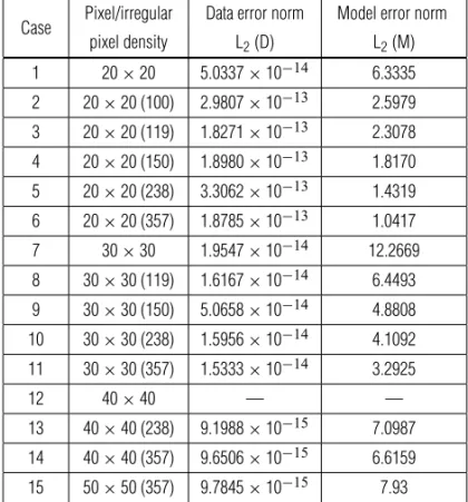
Inversion results. Data and model errors
Table 2 shows L2norms of Data and Model errors for several
ca-ses of matricesSp and Si. Minor the error, better the fitting. It is clearly seen that the data error is minimum in all cases, due to MLS method resolved the data perfectly. Therefore, the model error column defined the fitness quality of the inversion.
Considering, for example 20×20 pixel and ipixel sc matrices to form respectivelySp and Si and resolve the inversion, it was appreciated (Table 2, Cases 1-6):
Table 2 – Inversion results. Data and model errors.
Case Pixel/irregular Data error norm Model error norm
pixel density L2(D) L2(M) 1 20 × 20 5.0337 × 10⁻¹⁴ 6.3335 2 20 × 20 (100) 2.9807 × 10⁻¹³ 2.5979 3 20 × 20 (119) 1.8271 × 10⁻¹³ 2.3078 4 20 × 20 (150) 1.8980 × 10⁻¹³ 1.8170 5 20 × 20 (238) 3.3062 × 10⁻¹³ 1.4319 6 20 × 20 (357) 1.8785 × 10⁻¹³ 1.0417 7 30 × 30 1.9547 × 10⁻¹⁴ 12.2669 8 30 × 30 (119) 1.6167 × 10⁻¹⁴ 6.4493 9 30 × 30 (150) 5.0658 × 10⁻¹⁴ 4.8808 10 30 × 30 (238) 1.5956 × 10⁻¹⁴ 4.1092 11 30 × 30 (357) 1.5333 × 10⁻¹⁴ 3.2925 12 40 × 40 — — 13 40 × 40 (238) 9.1988 × 10⁻¹⁵ 7.0987 14 40 × 40 (357) 9.6506 × 10⁻¹⁵ 6.6159 15 50 × 50 (357) 9.7845 × 10⁻¹⁵ 7.93
Note: 20×20 (100) means medium with 20×20 ip made from previous 100×100 p.
Table 3 – Model parameters.
Case Pixel/irregular Vhost Vinc Xinc Yinc Width Height
pixel density (m/s) (m/s) (m) (m) (m) (m) True 400 2000 0.595 0.784 0.238 0.224 1 20 × 20 — — — — — — 2 20 × 20 (100) 331 2182 0.58 0.76 0.22 0.17 3 20 × 20 (119) 329 2002 0.59 0.74 0.22 0.20 4 20 × 20 (150) 341 2014 0.59 0.76 0.21 0.17 5 20 × 20 (238) 348 2163 0.59 0.74 0.23 0.21 6 20 × 20 (357) 359 1911 0.59 0.75 0.22 0.20 7 30 × 30 — — — — — — 8 30 × 30 (119) 294 3102 0.631 0.801 0.292 0.242 9 30 × 30 (150) 305 2177 0.591 0.812 0.264 0.190 10 30 × 30 (238) 327 2223 0.586 0.797 0.299 0.229 11 30 × 30 (357) 335 2172 0.590 0.815 0.230 0.190 12 40 × 40 — — — — — — 13 40 × 40 (238) 308 2879 0.58 0.76 0.24 0.16 14 40 × 40 (357) 318 4453 0.60 0.76 0.18 0.14 15 50 × 50 — — — — — — 16 50 × 50 (357) 311 4680 0.60 0.815 0.223 0.151
(a) (b)
(c) (d)
Figure 7 – Inversion results from ip. (a) 20×20(119): ip from previous 119×119 uniform pixels; (b) 20×20(238) ip.; (c) 30×30(238) ip.; (d) 50×50(357) ip. a) The fact to divide the medium in pixels of the same size
increase the model error of the inversion, as it is seen in case 1 respect to 2-6.
b) Considering now only cases 2-6; the model error decre-aseswhen more number of former pixel were considered to construct the subsequent ipixel Simatrix. For example consider the cases when those were 100×100 pixel with Me=2.5979; and 357×357, that brought a Me=1.0417. Probably this is related to an increase in precision to eva-luate the ipixels.
c) Denser the originalSc matrixand coarser the ipixel Sc
derived from it; will signify that minor will be the spatial
coverage difference between the ipixels. Conversely, coar-ser the former pixel matrix, more difficult will be to obtain precision in the evaluation of the irregular pixels. d) The analysis made above is demonstrated again, in cases
7 and below.
CONCLUSIONS
The MLS method functioned properly when the spatial coverage was uniform (as it was in all ipixel cases), bringing to accepta-ble results inclusive when the density of ipixels was very high. In all the other cases with pixels conforming the different raypath matrices, it was impossible to obtain a convergence to a solution.
The best inversion results were obtained with a maximum number of 20×20=400 ipixels, that is four times the data number (i.e. number of measurements). Although it is possible to obtain a solution with greater ipixel densities, neverthelessdiminishes the spatial resolutionof the image. In these cases and if the ipixel size is important to image a smaller inclusion, will be necessary to add additional information (such as a vector of background velocities
V host) to get a better image.
Finally, it was demonstrated that (at least in MLS) using ip improves convergence in the inversion process.
ACKNOWLEDGEMENTS
This work has been partially supported byConsejo de Investiga-ciones Cient´ıficas y Tecnol´ogicas (CICITCA); Universidad Nacio-nal de San Juan, Argentina.
REFERENCES
BRANHAM RL. 1990. Scientific Data Analysis. An Introduction to Over-determined Systems. Springer Verlag. NY. 237 pp.
FERNANDEZ AL. 2000. Tomographic Imaging the State of Stress. PhD Dissertation. Georgia Institute of Technology. Atlanta. USA. 298 pp. GOLUB GH & VAN LOAN CF. 1989. Matrix Computations. Baltimore: John Hopkins University Press, 642 pp.
IMHOF AL. 2007. Caracterizaci´on de Arenas y Gravas con Ondas El´asticas: Tomograf´ıa S´ısmica en Cross-Hole. PhD Thesis. Universidad Nacional de Cuyo. Mendoza. Argentina. First Prize Award Fundaci´on Garc´ıa Si˜n´eriz for the Best Doctoral Thesis in Pure or Applied Geophys-ics. XIV Convocation. Universidad Polit´ecnica de Madrid. 299 pp.
IMHOF A & CALVO C. 2003. A Variational Formulation to Image Inclu-sions in 2D Travel Time Cross-Hole Tomography. Brazilian Journal of Geophysics, 21(3): 269–274.
KOLSKY H. 1963. Stress Waves in Solids. Dover Publications Inc. NY. 213 pp.
MENKE W. 1989. Geophysical Data Analysis: Discrete Inverse Theory. Academic Press, Inc. NY. USA. 289 pp.
PENROSE RA. 1955. A Generalized Inverse for Matrices. Proceedings of Cambridge Phil. Society, 51: 406–413.
SANTAMARINA JC & CESARE MA. 1994. Velocity Inversion in the Near Surface: Vertical Heterogeneity and Anisotropy. Internal Report. Univer-sity of Waterloo. Canada.
SANTAMARINA JC & REED AC. 1994. Ray Tomography: Errors and Error Functions. Journal of Applied Geophysics, 32: 347–355. SANTAMARINA JC & FRATTA D. 1998. Introduction to Discrete Signals and Inverse Problems in Civil Engineering. ASCE Press. USA. 327 pp. SANTAMARINA JC, KLEIN KA & FAM MA. 2001. Soils and Waves. Wiley & Sons. Ltd. England. 488 pp.
SHERIFF RE & GELDARD LP. 1995. Exploration Seismology. 2ndEdition.
Cambridge University Press, NY. 592 pp.
STRANG G. 1980. Linear Algebra and Its Applications. Academic Press, NY. 414 pp.
TARANTOLA A. 1987. Inverse Problem Theory. Elsevier. Amsterdam. 613 pp.
TARANTOLA A. 2005. Inverse Problem Theory and Model Parame-ter Estimation. Society for Industrial and Applied Mathematics. SIAM. Philadelphia. USA. 333 pp.
NOTES ABOUT THE AUTHORS
Armando Luis Imhof. Geophysicist graduated at Universidad Nacional de San Juan (UNSJ, Argentina) in 1989. Specialist on Environmental Studies from
Universidad Nacional de San Luis (Argentina), 2002. PhD degree from Engineering Faculty at Universidad Nacional de Cuyo, Mendoza, Argentina, 2007. First Prize winner of XIV Convocation, Garc´ıa Si˜n´eriz Foundation (Spain) to the Best PhD Thesis in Geophysics from Spain and Latin America. Researcher from the staff of Instituto Geof´ısico Sismol´ogico Volponi (Facultad de Cs. Exactas, Fcas y Naturales – UNSJ) and Adjoint Professor of the asignature Electrical Prospecting, Geophysics and Astronomy Department (UNSJ) since 1990. Member of Asociaci´on Argentina de Geof´ısicos y Geodestas (AAGG). Topics of main Research: Geophysics applied to mining, geotechnics and hidrogeological studies.
Carlos Adolfo Calvo. Electromechanical Engineer graduated at Universidad Nacional de San Juan (UNSJ, Argentina) since 1978. MSc in Applied Mathematics and
Informatics from Moscow Physics Institute (MEPHI). Main Professor of the asignatures Mathematics Analysis, Applied Mathematics and Numerical Methods; Engineering Faculty (UNSJ). Researcher on topics covering applied mathematics to solve engineering problems. Topics of main research: Applied mathematics.
Juan Carlos Santamarina. Civil Engineer from Universidad Nacional de C´ordoba, 1982; MSc in Geotechnical Engineering at University of Maryland, 1984. PhD in
Geotechnical Engineering at Purdue University, 1987. Co-director at the Center for Applied Geomaterials Research (Georgia Institute of Technology); Goizueta Foundation Professor at Georgia Institute of Technology, Atlanta, USA.