i
Credit Risk Modelling using Multi-state Markov Models
João Paulo Nogueira Santos
A Dissertation as a partial requirement to obtain the degree of Master in Statistics and Information Management, specialization in Risk Analysis and Management
1
NOVA Information Management School
Instituto Superior de Estatística e Gestão de Informação
Universidade Nova de LisboaCREDIT RISK MODELLING USING MULTI-STATE MARKOV MODELS
by
João Paulo Nogueira Santos
A Dissertation as a partial requirement to obtain the degree of Master in Statistics and Information Management, specialization in Risk Analysis and Management
Mentor: Prof. Doctor Jorge Miguel Ventura Bravo
2
ACKNOWLEDGMENTS
I would like to thank my advisor for the opportunity to work with multi-state models and their implementation in other research areas, more specifically the financial area.
To my family, for the support and love during my 27 years of life. Especially to my mom, a woman who I am very proud of and who did everything in her power to allow me to lead the life I have today.
3
SUMMARY
This paper is devoted to credit risk modelling issues concerning mortgage commercial loans. Mortgage loans are one of the most popular type of loans provided by credit institutions. Like in the case of other loans, the main concern of institutions providing this type of product is a potential inability to recover the amount assigned to their clients (credit risk). In order to prevent possible losses for credit institutions resulting from clients entering in default, it is therefore crucial to study the behaviour of risky clients. This issue can be addressed through several models, namely through the multi-state Markov model, despite it constituting a more unusual approach in the context of dealing with credit risk modelling. The multi-state Markov model is a useful way of describing a process in which an individual moves through a series of states (finite number) in continuous time. By fitting this model to the loans of risky clients, it is possible to estimate the mean sojourn time in each state before a transition occurs, as well as the transition probabilities between the different states assumed by the contracts, therefore providing a relevant modelling framework for event history data. The present work relies upon 2008-13 databases from one of the biggest American companies that act in the secondary mortgage market, the Fannie Mae. Results show that with the application of the multi-state Markov model, contracts signed during 2013 are more propitious to a scenario of recovery when compared to those referring to the year 2008.
KEY WORDS
4
INDEX
1.
Introduction ... 6
2.
Literature review ... 9
3.
Methodology ... 13
4.
Results ... 18
5.
Conclusion ... 25
6.
Bibliography ... 26
5
LIST OF TABLES
Figure 1 – Multi-state model for loans progression ... 14
Figure 2 – Transition matrix for the proposed model ... 15
LIST OF TABLES
Table 1 – Definition of the states ... 15
Table 2 – Number of contracts for the periods of 2008-13 ... 17
Table 3 – Loan’s average time in the portfolio for the periods of 2008-13 ... 17
Table 4 – Percentage of contracts for the periods of 2008 ... 18
Table 5 – Percentage of contracts for the periods of 2013 ... 18
Table 6 – Transition intensities matrices for the periods of 2008 ... 19
Table 7 – Transition intensities matrices for the periods of 2013 ... 19
Table 8 – Mean sojourn times for the periods of 2008 ... 20
Table 9 – Mean sojourn times for the periods of 2013 ... 20
Table 10 – 1 year estimated transition probabilities for the periods of 2008 ... 21
Table 11 – 1 year estimated transition probabilities for the periods of 2013 ... 21
Table 12 – 2 year estimated transition probabilities for the periods of 2008 ... 22
Table 13 – 2 year estimated transition probabilities for the periods of 2013 ... 22
Table 14 – Number of active contracts observed in June 2015 ... 23
Table 15 – Estimated number of contracts in each state in June 2016 and June 2017 for the
portfolios of 2008-13 ... 24
LIST OF ABBREVIATIONS
FMNA Federal National Mortgage Association
GSE Government Sponsored Enterprise
MBS Mortgage Backed Securities
6
1. INTRODUCTION
Credit risk is the largest risk faced by commercial banks and is of concern to a variety of stakeholders: institutions, consumers and regulators. Credit risk may be defined as the risk of losses due to credit events, i.e. default (an obligor being unwilling or unable to repay its debt) or a change in the quality of the credit (rating change). Examples of default events include bond defaults, corporate bankruptcy, credit card charge-off and mortgage foreclosure. Other forms of credit risk include repayment delinquency in retail loans, loss severity upon the default event, as well as the unexpected change of credit rating. Credit risk modelling assists banks in estimating the expected loss (EL) on a credit exposure over a given time horizon, enabling institutions to price credit risks more effectively and to calculate how much capital has to be set aside as a provision. Credit expected losses depend in a multiplicative way on the Probability of Default (PD), on the Exposure at Default (EAD) and on the Loss Given Default (LGD).
Broadly speaking, credit risk models can be classified into two types based on the definition of credit loss. First, Default Mode (DM) models (also called as “two state” models) recognize credit loss only if a borrower defaults within the planning horizon. This means that in such models only two outcomes are relevant – non-default and default. If no default occurs, the credit loss is obviously zero. If default occurs, EAD and LGD must be estimated. In contrast, “multi-state” (or “mark-to-market”, MTM) models recognize that ‘default’ is the only one of the several possible credit rating grades to which the instrument could migrate over the planning horizon. As such, these models estimate the probability that the borrower's credit quality deteriorates (credit migration), including a change to default status. The MTM paradigm recognizes that there can be an economic impact even if the borrower does not default. A "pure" MTM approach would take market-implied values in different non-defaulting states. In real market applications, because of data and liquidity issues banks tend to use internal prices based on credit loss experiences.
The two main approaches in the MTM paradigm are the discounted contractual cash flow (DCCF) approach and the risk-neutral valuation (RNV) approach. In the DCCF approach, the current value of a non-defaulted loan is measured as the present value of its future cash flows, computed using market-determined or internal credit spreads for obligations of the same grade. The future value of a non-defaulted loan is dependent on the risk rating at the end of the time horizon and the credit spreads for that rating. The RNV approach is derived from option pricing theory. Prices are an expectation of the discounted future cash flows in a risk-neutral market.
Federal National Mortgage Association (FNMA), commonly known as Fannie Mae, is a government-sponsored enterprise (GSE)1 founded in 1983 whose mainly purpose is to provide liquidity in the secondary mortgage market2 in order to make possible for banks, insurance companies and mortgage banking companies to issue more mortgages than those would be able to issue with their own funds. Its activity encompasses four primary areas in the Single-Family Credit Guaranty business: (i) Mortgage Acquisitions, facilitating the purchase of single-family mortgage loans, generally for the
1 GSEs are “privately owned financial institutions established by the government to fulfill a public mission” – see
Congressional Budget Office, December 2010.
2 After a lender originate a mortgage loan, he can sell it in the secondary market to the investors in order to get available
7 purpose of securitizing them; (ii) Mortgage Securitization of single-family mortgage loans delivered to Fannie Mae MBS in lender swap transactions; (iii) Credit Risk Management, setting and maintaining standards for origination and servicing; and (iv) Credit Loss Management, preventing foreclosures and reducing costs of defaulted loans through foreclosure alternatives, management of foreclosures and real estate owned (REO) properties, and by pursuing contractual remedies from lenders, servicers, and providers of credit enhancement.
Like commercial banks, Fannie Mae can generate profits by lending money. In its activity, Fannie Mae “buys” mortgage loans, consequently assuming the credit risk associated with these loans. Credit risk is present throughout the entire life cycle of contracts, starting with the granting of credit, followed by their monitoring and potentially ending up in situations of non-compliance, with the process of credit recovery. In this way, Fannie Mae, like other financial institutions, is exposed to default risk, defined as the failure of a borrower to meet its contractual obligations to repay a debt in accordance with the agreed terms.
In 2008-09, the United States entered into the deepest recession since the Great Depression of 1929-33. Although noticeably similar, the depth of integration between modern global financial centers exacerbated the effects of this recession, therefore triggering a global crisis. Although there is still much research to be done, the residential mortgage lending practices in the United States were in the root of the shock (Demyanyk and Otto, 2011). Many of the financial products created during the period leading up to the crisis, enabled by the process of securitization, played a central role in the development of the sub-prime mortgage industry. The products were ambiguous; the underlying risk was difficult to picture and hence, price. The primary products that enabled the financing of the sub-prime market segment were Mortgage Backed Bonds (MBB's) and Collateralized Mortgage Obligations (CMO's). These products effectively package pools of mortgage debt into the form of a bond which could then be sold on the investment market. These bonds offered investors higher than average yields when compared to existing straight bonds such as Treasury bonds and corporates and provided the liquidity necessary to keep financing the U.S. real estate market. On September 7, 2008, the federal government took control of Fannie Mae. The company was put in conservatorship (a statutory process with the objective of restoring the financial strength of the company in order to ensure its solvency), under the terms and supervision of FHFA3, and remains in this situation to the present day4.
Given the importance of default risk for financial institutions, which in more severe cases can result in bankruptcy, it is fundamental to ensure an efficient management of credit portfolios based on modern methodologies of quantification of risk, as well as a more traditional credit risk analysis, through which customers credit profile are evaluated.
This paper aims to contribute to the current literature on this topic by developing a modelling approach specifically to discuss loan performance during 2008-13, using data on mortgages acquired by Fannie Mae. As a whole, it seeks to answer the following 2 main questions:
1. What is the main contribution of multi-state Markov models in credit risk modelling;
3 ”FHFA is a member agency of the Financial Stability Oversight Council. The Council is charged with identifying risks to the
financial stability of the United States; promoting market discipline; and responding to emerging risks to the stability of the United States' financial system” – see http://www.fhfa.gov/AboutUs.
8 2. Are there significant differences in the loan performance for Fannie Mae portfolios of
2008-13.
Taking into account how clients can behave throughout the life cycle of their loans, this study aims to analyse the transition probabilities between the different states that a contract can assume, by resorting to a model less traditionally adopted for credit risk modelling, namely the multi-state Markov model. Not only are there few references in existing literature regarding the applicability of this model in the financial sector, but also it can be considered that this method represents an important approach to define contracts’ movement, given that it renders it possible to estimate the probability of a contract moving to a certain state based on its present position. The scope of this work also includes an estimate of the mean sojourn time in each transition state, the 1 and 2 year transition probabilities, as well as a comparison of the results of 2008-13. Additionally, there is also an analysis of the application of the multi-state Markov model in these two periods, given that in 2008 we are faced with Fannie Mae crisis, while in 2013 represents a relatively more recent period to study, based on which it is possible to understand if the credit portfolios of Fannie Mae represent comparatively more or less risk to the institution. Although the variables included in the data set are discrete, this study relies on the application of multi-state Markov model in continuous time once that this model provide an important contribute in terms of time prediction of the possible transitions. Multi-state models are also used by considering covariates, in order to study the relation of constant or time-varying characteristics of individuals with their transition rates. Although this is a possible approach to the issue at hand, this work does not focus on a simulation of models with these types of characteristics.
Taking into account all of the above mentioned analysis, this paper is organized as follows. In section 2 we illustrate the literature review about the company under study, a sample of models used in credit risk modelling and the utility of the multi-state model in the observation of an individual. In section 3, the methodology of the multi-state Markov model, as well as the data used in the estimation of the model are presented. Finally, in section 4, the results from the implementation of the model are addressed, while in section 5 the overall conclusions of this work are presented.
9
2. LITERATURE REVIEW
Credit risk models are critical in risk management as a mechanism to address issues such as qualifying aggregate credit risk, identifying concentration risk, quantifying marginal risk, i.e., the effect on portfolio risk on account of the addition of a single asset, setting risk limits, and quantifying economic and regulatory capital.
Traditionally, credit risk models can be divided into three main categories: (i) reduced-form models, (ii) “first generation” structural-form models, (iii) “second generation” structural-form models. Reduced form models do not attempt to explain default events. Instead, they concentrate directly on modelling default probabilities. As such, default events are assumed to occur unexpectedly due to one or more exogenous events (observable and unobservable), independent of the borrower's asset value. Observable risk factors include changes in macroeconomic factors such as GDP, interest rates, exchange rates or inflation, whereas unobservable risk factors are specific to a firm, industry or country. Individual level reduced form models were first proposed by Altman (1968), who founded the quantitative credit analysis literature. The author proposes discriminant analysis to determine combinations of observable characteristics that may best differentiate between defaulted and non-defaulted firms. The credit scoring model developed by Altman (1968), broadly known as the “Z-Score Model”, proposes a discriminant model including five statistically significant financial ratios to predict corporate bankruptcy by assigning a Z-score to an obligor.
After obtaining this score for a sample of manufacturing firms, the author concludes that all the companies with a Score lower than 1.81 fall into the bankruptcy group, while companies with Z-Scores higher than 2.99 correspond to the non-bankruptcy group. Z-Z-Scores in-between correspond to the “zone of ignorance”, though the author then concludes that the value that best separates both groups is 2.675. Altman, Haldeman and Narayanan (1977) developed an alternative seven-variable model called “ZETA Model”, which they proved to be more effective in forecasting bankruptcy for 2-5 years horizons. After its proposal, many models based on credit scoring system have been widely used in credit risk analysis. Altman and Narayanan (1997) analysed various predictor variables in order to identify the most significant ones on the event of default and found that indicators related to profitability, liquidity and leverage were the most representative.
Besides discriminant analysis linear probability models, alternative credit scoring models are widely used to measure default risk in consumer lending. Alternative methodologies include Logit models (Martin, 1977), Probit models (Ohlson, 1980), Multiple discriminant analysis models, Decision trees, Survival analysis (Kleinbaum and Klein, 2012), Neural Networks and Least Square Support Vector Machines (Chen et al. 2012). Credit scoring is useful for banks and other lending institutions for two main purposes, namely initial scoring and behaviour scoring (Chamboko and Bravo, 2016). Initial scoring provides a basis for lending institutions to score new credit applicants, in order to decide on whether to grant a loan to an applicant, and as well to estimate the down payment and interest rates for different clients. On the other hand, behavioural scoring models are those which allow institutions to predict the repayment behaviour or performance of their clients for purposes of capital management, customer relationship management, profitability forecasting, setting risk based collections and recovery strategies among other reasons (see, e.g., Malik and Thomas, 2012).
10 Logistic regression does not assume that the independent variable is normally distributed and is capable of generating predicted probability estimates. Intuitively, logistic regression was very appealing to the credit risk assessment task since traditional models were only aimed discriminating bad and good potential obligors. The main advantage of logistic regression is the fact that it is a non-parametric classification technique, as no prior assumptions are made with regard to the probability distribution of the given attributes.
Artificial Neural Networks are computational methods that use a large set of elementary computational units, called neurons, to solve problems mimicking the behaviour of human brain (Russell and Norvig, 2010). In turn, a decision tree method is a non- parametric approach which uses a decision tree to map observations of an individual to conclusions about the individual’s class. The major problem associated with this technique is over fitting, a problem solved by the use of random forests (Imielinski and Mannila, 1996).
The quantitative “credit-scoring” approach to credit risk modelling continues to be widely used in the financial system but lost some of its appeal in recent decades, partly because of its descriptive focus. Discriminant analysis characterizes a firm’s likely observable characteristics given the current default status, while a credit analyst is usually interested in knowing the individual's or firm’s likely default status given its observable characteristics. Moreover, Lo (1986) proves that discriminant analysis is consistent in a much more limited set of circumstances relative to other, more modern approaches. One such approach is logistic regression models that explore a methodology to directly estimate the effects of particular variables on default probabilities (or in the case of logistic regression, the log odds-ratios of the default probabilities).
The first generation structural-form models (SFM) are based on the original option pricing framework developed by Merton (1974). In such a framework, the default process of a company is driven by the value of the company’s assets and the risk of a firm’s default is explicitly linked to the variability in the firm’s asset value. More specifically, Merton derived a formula to estimate the probability of default (PD) by assuming the firm issues a zero-coupon bond that represents its entire debt. In this model the PD is equivalent to the probability that the value of the firm's assets are less than the face value of a given bond, or similarly, the probability that market value of a firm is lower than its liabilities. According to these models, all relevant credit risk elements, including default probabilities and recovery rates (RR) at default are linked to the structural characteristics of the firm: firm's assets and asset volatility (business risk) and leverage (financial risk). Asset values are inferred from equity prices. The Merton model has been developed subsequently and modifies the original model by relaxing one or more of its assumptions. Black and Cox (1976) provide a more complete and realistic model by analysing firms with complex structures of capital and debt. Geske (1977) extended the model to a bond in which interest is paid periodically and default events can happen either at maturity time or every time the coupon is paid, while Vasicek (1984) differentiates between short and long term debts.
Also, first generation structural-form models assume that default can occur only at maturity of the debt when the firm’s assets are no longer sufficient to cover debt obligations. Differently, second generation structural form models assume that default may occur at any time between the issuance and maturity of the debt, when the value of the firm’s assets reaches a given lower threshold level (see, e.g., Kim, Ramaswamy, and Sundaresan, 1993; Hull and White, 1995; Longstaff and Schwartz,
11 1995). This approach simplifies the first class of models by both exogenously specifying the cash flows to risky debt in the event of bankruptcy and simplifying the bankruptcy process. This contrasts with reduced-form models that do not condition default on the value of the firm, and parameters related to the firm’s value need not be estimated to implement them. Jones, Mason and Rosenfeld (1984) and Shumway and Bharath (2008), among others, investigated the reasonableness of the key structural assumptions of these models with fairly disappointing results. The authors demonstrate that structural models are outperformed by reduced form models to such an extent that it is possible to outperform Merton (1974) and its modern-day implementations both in-sample and out-of-sample with a much simpler alternative that does not require the stringent assumptions or simultaneous non-linear equations of the structural approach. Duffie and Lando (2000) concluded that is better to use an approach based on a multistate system that estimates the default event before it occurs instead of using structural-form models.
The third generation of the structural-form models are the credit value-at-risk (VaR) models, very popular in credit risk analysis and management (see, e.g., J.P Morgans CreditMetric, 1997; Moody's KMV model; Credit Suisse Financial Products Credit Risk+, 1997; Mckinseys CreditPortfolioView, Wilson, 1998). In particular, CreditMetrics and KMV models are analytically based on Merton model and therefore use has key data sources for the analysis both corporate assets’ value and assets’ volatility. In the case of CreditRisk + method, the most important sources are default risk level and its volatility. Moody’s KMV method determines a credit event as a change in distance to default, which subsequently leads to changes in the EDF (Expected Default Frequency) value. This model has been developed to provide a term structure of default risk probabilities. The term “Distance-to-default” is proposed in this KMV model, and it calculated based on the market asset value of the firm, its volatility and the default point term structure, which altogether allow for the quantification of actual probability of default (Sreedhar and Shumway, 2004).
It should be noted that traditional two-state credit risk models, which describe the full loss distribution by the distribution of number of defaults in portfolio, tend to neglect migration risk and recovery rate. Contrarily, in a multi-state model, we do not constrain the possible credit events to just two, default or no default, but instead we also model changes in credit quality, along with their effects on the market value of the instruments in the portfolio and systematic/unsystematic recovery risk. Apart from estimating the probability of the transition from a non-defaulting state to defaulting state over a certain period of time, other kinds of transitions are not considered. It is known that there are several possible states in the relationship between clients and financial companies, such as non-defaulting without revolving credit use, non-defaulting with revolving credit use, in delay, voluntary cancellation and default. Customers pass through these states over time, and this is a characteristic of recurrent events. As such, the existence of several possible states demands the use of multi-state models.
Trench et al. (2003) developed a markovian decision process in order to guide a bank in determining price and credit lines for credit card holders in order to maximize profits. In turn, So and Thomas (2010) used Markov chain modelling transition probabilities in logistic models in order to evaluate credit risk of credit card portfolios. So and Thomas (2010) also use a Markov chain model for revolving consumer credit accounts based on consumers' behavioural scores that includes the impact of the economy on the risk migration of credit card accounts. The models show how economic variables such as unemployment and price indexes have an impact in credit risk, both directly, by
12 changing the dynamics of the credit scores, and indirectly, by affecting how many credit card accounts become inactive or reactive themselves. Malik and Thomas (2012) develop a Markov chain model based on behavioural scores for establishing the credit risk of portfolios of consumer loans. In sum, multi-state models credit operations can assume different states (for example, non-defaulting, in delay, defaulting) through time. Some of these states are temporary, i.e. the individual can leave this state at some time (for instance, an individual in delay can go back to a non-defaulting situation) and others are absorbent, i.e. once in this state, the individual cannot migrate to another state (for instance, a defaulting individual leaves the individual database and cannot take on another state). The Multi-state Markov model assumes that the transition probabilities among states depends only on the time between transitions and on the covariates (which are eventually time dependent) associated to the individuals.
There are many variations of multi-state models. For instance, a two-state model for survival data only considers 2 states and one possible transition, from state 0 to state 1. The competing risk model is based on one transient (temporary state) state, 0 and a number, k, of absorbing (final) states. In turn, illness-death models take in consideration that an individual may change status before the absorbing event, which means that an individual may switch between two states before it reaches the final state. Finally, there are hidden Markov models (HMM), where the states of the Markov chain are not observed. Instead, the observed data is governed by some probability distribution (the emission distribution) conditional on the unobserved state. It should be noted that this work does not aim to present in depth the assumptions or the methodology for each type of model. For this purpose, we recommend a review of Statistical Models Based on Counting Processes (1993), where Andersen P.K. provides a more extensive overview of these models and more general event history analysis.
13
3. METHODOLOGY
So far this study has presented the company under analysis, a literature review about credit risk modelling, and a proposal of modelling the transitions between states for the Fannie Mae loans. This following section now presents the complete methodology behind the chosen model, as well as an overview of the data set treatment performed for the proposed analysis, which was developed in R using the msm package.
3.1. Credit Data Set
The primary data source used for this study was the Fannie Mae's Single Family Loan Performance Data Set. This data includes both borrower and loan information at the time of origination, as well as data on the loan's performance. There is no information from Fannie Mae regarding which of the loans in the dataset are still active, but it is assumed that if a loan is part of the data set until the last month of observation (June 2015) this loan is active. The remaining loans were assumed to have closed at any time in the past, due to a credit event (for instance, a repurchased or short sell).
Fannie Mae separates the mortgage loan credit performance data into two files for each acquisition quarter, starting in 2000: Acquisition and Performance. The Acquisition file contains the variables which encode the borrower and loan characteristics. Examples of these include Borrower Credit Score, Original Interest Rate, Property Type and Original Combined Loan-to-Value. The Performance file tracks loan performance characteristics. Examples of these variables include current loan delinquency status, month-to-month payment history, loan age, mortgage servicer, and maturity date of the loan. Each loan has a unique Loan Identifier which links the Acquisition file to the Performance records. In both files the data presented for each quarter regarding loans acquired is independent from data for another quarter, and therefore it is only possible to consult the entire history of a loan in one quarter5.
With respect to information at the time of origination, the data includes the borrower's credit (FICO) score, the date of origination, the loan size, the loan size relative to the house value (LTV ratio), whether the loan is originated for purchase or refinancing, the three-digit zip code of the property, and the interest rate on the mortgage. The loan performance data is provided monthly and includes information on the loan's age, the number of months to maturity, the outstanding mortgage balance, whether the loan is delinquent, the number of months it has been delinquent and whether the loan is prepaid. There is an unique loan identifier code in the data set that allows a loan to be tracked from inception through its subsequent performance.
In total, the data set includes 1.518.579 loans which were purchased by Fannie Mae in the first half of 2008-13, whose performance is tracked from January 2008 to June 2015 (contracts of 2008) and January 2013 to June 2015 (contracts of 2013). The loans were purchased from originating lenders and represent mortgages originated throughout all the states of the United States. The loans are all 30-year, fully amortization, full documentation, conventional fixed-rate mortgages.
5 In the Fannie Mae data, a quarter of a given year isn’t represented by 3 months of observation of the loans, but by the set
14 To accomplish this project, a combination of SAS Enterprise guide and R software was used. The first was employed in the analysis of the data sets provided by Fannie Mae, while the preparation of the data in order to fit the multi-state Markov model was performed in R software.
3.2. Multi-state Markov model
In order to model the transitions from one state to another it is necessary to define a multi-state model, while taking into consideration the particularities of the available data sets. With this purpose, the possible number and type of transitions between states, together with the available states for the individuals should be analysed. Some of these states are temporary, i.e. the individual can leave this state at some time (for instance, an individual in delay can go back to a non-defaulting situation) and others are absorbent, i.e. once in this state, the individual cannot migrate to another state (for instance, a defaulting individual leaves the individual database and cannot take on another state). In the application of multi-state models there is also the possibility of integrate covariates to study the relation of constant or time-varying characteristics of individuals to their transition rates. Although this is one possible approach, the current work will not focus on simulating models with these type of characteristics.
In studies where multi-state models are applied, the Markov assumption is commonly adopted. This assumption relies on the premise that future evolution only depends on the current state, and previous states are not involved in the subsequent transition probabilities. In mathematical terms, 𝑞𝑞𝑟𝑟𝑟𝑟(𝑡𝑡; 𝑧𝑧(𝑡𝑡); 𝐹𝐹𝑡𝑡) is independent of 𝐹𝐹𝑡𝑡, the observation history 𝐹𝐹𝑡𝑡 of the process up to the time
preceding t. See, for example, Cox and Miller (1965) for a thorough review of continuous-time Markov chain theory.
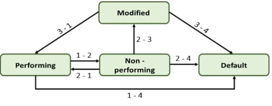
Figure 1 – Multi-state model for loans progression
Source: the author.
For the purpose of this study, the implementation of the model was performed via msm, a package of functions for multi-state modelling based on R statistical software. Taking into consideration the nature of the data, the allowed movements between different states were defined according to figure 1, and included 4 different states. The arrows show which transitions6 are possible between states, which are defined as follows:
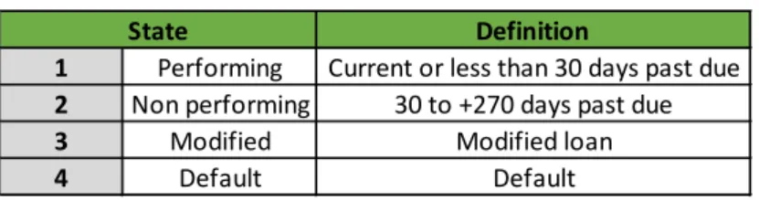
15 Table 1 – Definition of the states
Source: the author.
The next state to which the individual moves, and the time of the change, are governed by a set of transition intensities 𝑞𝑞𝑟𝑟𝑟𝑟(𝑡𝑡, 𝑧𝑧(𝑡𝑡)) for each pair of states r and s. The intensities may also depend on
the time of the process 𝑡𝑡, or more generally, on a set of individual-specific or time-varying explanatory variables 𝑧𝑧(𝑡𝑡). The intensity represents the instantaneous risk of moving from state r to state s and is given by:
𝑞𝑞𝑟𝑟𝑟𝑟�𝑡𝑡, 𝑧𝑧(𝑡𝑡)� = lim𝛿𝛿𝑡𝑡→0𝑃𝑃(𝑆𝑆(𝑡𝑡 + 𝛿𝛿𝑡𝑡) = 𝑠𝑠|𝑆𝑆(𝑡𝑡) = 𝑟𝑟/𝛿𝛿𝑡𝑡
The intensities form a matrix Q whose rows sum to zero, so that the diagonal entries are defined by 𝑞𝑞𝑟𝑟𝑟𝑟 = − � 𝑞𝑞𝑟𝑟𝑟𝑟
𝑟𝑟≠𝑟𝑟
To fit a multi-state model to the available data, a transition intensity matrix was estimated. The Markov assumption was that future evolution only depends on the current state. That is, 𝑞𝑞𝑟𝑟𝑟𝑟(𝑡𝑡, 𝑧𝑧(𝑡𝑡)𝐹𝐹𝑡𝑡) is independent of 𝐹𝐹𝑡𝑡, the observation history 𝐹𝐹𝑡𝑡 of the process up to the time
preceding t (Cox and Miller).
As a result, and according with the model definition for this work, the states may be modelled as a homogeneous continuous-time Markov process, with a transition matrix Q, pictured below:
Figure 2 – Transition matrix for the proposed model
Source: the author.
Kalbfleisch and Lawless, and later Kay, described a general method for evaluating the likelihood for a general multi-state model in continuous time, applicable to any form of transition matrix. The likelihood is calculated from the transition probability matrix 𝑃𝑃(𝑡𝑡). For a time-homogeneous process, the (𝑟𝑟, 𝑠𝑠)) entry of 𝑃𝑃(𝑡𝑡), 𝑃𝑃𝑟𝑟𝑟𝑟(𝑡𝑡), is the probability of being in state s at a time 𝑡𝑡 + 𝑢𝑢 in the future,
given the state at time u is r. It does not say anything about the time of transition from r to s, indeed the process may have entered other states between times u and 𝑡𝑡 + 𝑢𝑢. 𝑃𝑃(𝑡𝑡) can be calculated by taking the matrix exponential of the scaled transition intensity matrix (see, for example, Cox and Miller):
𝑃𝑃(𝑡𝑡) = exp (𝑡𝑡𝑡𝑡)
Definition
1 Performing Current or less than 30 days past due
2 Non performing 30 to +270 days past due
3 Modified Modified loan
4 Default Default
16
3.3. Estimation Procedure
As mentioned before, the mortgage loans provided by Fannie May for the first two quarters of 2008-13 were used in order to study the transition probabilities between states, through a multi-state Markov model. Since there are variations in these kind of models (as illustrated in the review literature chapter), an analysis of the variables provided by Fannie May was necessary, as well as some treatment to the information prior to the implementation of the model, already described previously.
The following variables of the dataset were used: 1) LOAN_ID: identifier of the contract;
2) LOAN_AGE: life period, in months, of the credit mortgages;
3) DELQ_STAT: state of a contract;
4) ZB_CODE (zero balanced code): a code indicating the reason the loan's balance was reduced to
zero or experienced a credit event. The possible codes7 are: • 01 = Prepaid or matured;
• 03 = Short sale, third party sales and other foreclosure alternatives; • 06 = Repurchased;
• 09 = REO disposition or deed-in-lieu.
Through the analysis of the variable “LOAN_AGE” it was identified that some contracts presented incomplete historical information, and will as a result not be eligible to enter the model. Also, there was a concern that some contracts could not have enough historical information. Based on the methodology used in credit scoring models, where the classification of an individual as “good” or “bad” is observed during a certain period of time, for the study at hand it was determined that contracts presenting less than 128 months of historical information would be excluded. Additionally, there were contracts where variable “LOAN AGE” was set to minus one. Since there was no evidence about the real initial date of these contracts, they were excluded from the final data set in order to ensure more reliable results.
With respect to the variable “DELQ_STAT”, we concluded that some contracts have transitions between states, namely from one month to the next, higher than 30 days (for instance, a contract in the present month has 30 days past due and in the following month presents 120 days past due). This variable, originally, was represented by 10 states, from the state 0 (current or less than 30 days past due), to state 9 (30 or +270 days past due). The other states were represented by intervals of 30 days past due (state 1, from 30 to 59, and so on). For this work we choose to modify the variable and define the state 1 as ”current or less than 30 days past due” and aggregate the remaining states into just one, namely state 2. Also, it was noted that in some instances the variable assumed a value “X” in the last date of observation of the contracts. When this occurred, the variable “ZB_CODE” was in some instances (not all) filled with one of the 4 codes presented before. Based on this, the state in this observation is modified: it is considered that when the “ZB_CODE” is “03” or “09” we are faced with a default situation and when is “01” or “06” we are faced with a performing situation (which can lead to a transition from performing to default). Also, when there is no code associated to the zero
7 The definition of the presented codes is based on the Fannie Mae guideline. 8 Period commonly used in credit scoring models in Portuguese banking.
17 balanced code variable and the penultimate position has the non performing state, it was assumed that the contract ends its lifetime cycle in a state of default.
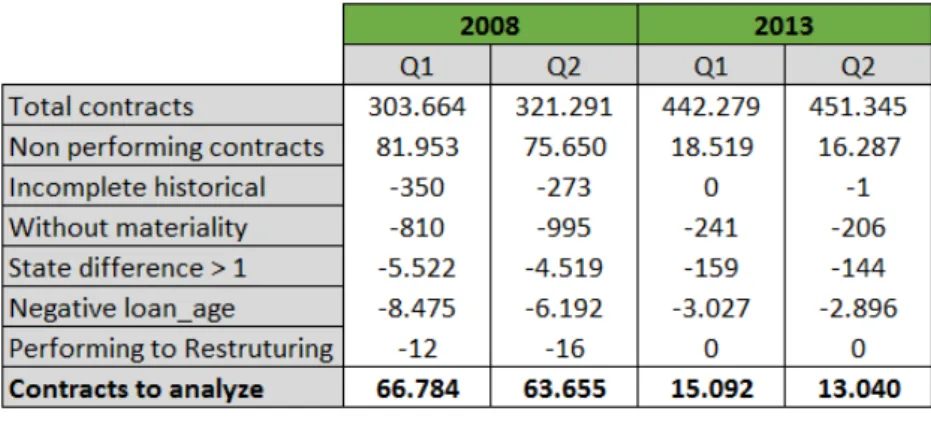
Table 2 below presents the number of contracts for each quarter of the years being analysed, as well as the number of contracts excluded based on the previously presented exclusion rules.
Table 2 – Number of contracts for the periods of 2008-13
Source: the author.
In turn, the loan’s average time in the portfolio for the contracts under analysis is presented below in table 3:
Table 3 – Loan’s average time in the portfolio for the periods of 2008-13
Source: the author.
Q1 Q2 Q1 Q2
37 36 14 13
18
4. RESULTS
This section presents the results from the implementation of the multi-state Markov model, including the analysis of the number of transitions between states (on a monthly basis), the transition intensities matrix, that illustrates the instantaneous risk of contracts moving from one state to other (with 95% confidence intervals), the estimated mean sojourn times in each transient state, the one and two years estimated transition probabilities and the future number of contracts in each state, applying these probabilities.
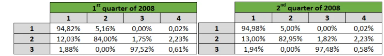
Table 4 and table 5 below present the percentage of contracts for each quarter of the years under analysis:
Table 4 – Percentage of contracts for the periods of 2008
Source: the author.
Table 5 – Percentage of contracts for the periods of 2013
Source: the author.
Taking in account the total number of observed transitions for each quarter, it is possible to conclude that state combination (1 – 1) is verified around 94% of the time. This means that 94% of the total number of transitions occurred when a contract in the present month of observation was in state 1 and continued in state 1 in the following month.
In analogous terms, looking at contracts initially in state 2, it can be concluded that in both quarters of 2008 circa 83% of the transitions occurred with contracts remaining in state 2 in the following month. In 2013 this number is considerably lower (about 42%), while the state combination (2 – 1) occurs 54% of the times, i.e., circa 54% of the total number of transitions occurs when a contract in the present month of observation is in state 2 and moves to state 1 in the following month. State combination (3 – 3) represents circa 97% and 80% of transactions for 2018 and 2013, respectively. Considering this state (state 3) as the state under observation, for 2013, 14% of transitions represent contract that move to state 1 in the following month.
The analysis presented above allowed for a better understanding of the data sets used in this work, namely that these include contracts that remains most of the times in the same state. However, it was also possible to conclude that a considerable number of transitions occur when a contract is in state 2 and moves to state 1 in the next month.
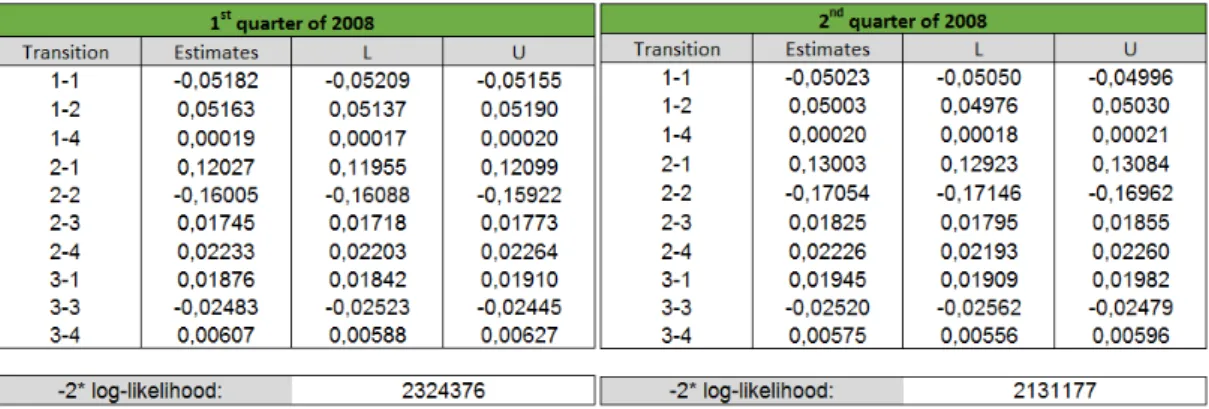
19 Table 6 – Transition intensities matrices for the periods of 2008
Source: the author.
Table 7 – Transition intensities matrices for the periods of 2013
Source: the author.
By looking at the transition intensities matrices for the period of 2008 presented above, it is possible to conclude that there is a low instantaneous risk for the contracts to move from state 1 to state 2 which is even lower when we analyse the transition to state 4. For contracts initially in state 2, the instantaneous risk of movement from state 3 to 4 is very similar (approximately 1,8% and 2,2%, respectively), while a higher value is observed in state 1 (12% and 13%). For contracts initially in state 3, we conclude that there is a minimum risk of movement to states 1 and 4 (1,9% and 0,6% respectively). The results for 2013 largely contrast with those for 2008, where the possibility of recovery from state 2 to state 1 is noticeable. Although this tendency exists in both years, in 2013 the possibility of this transition is higher than 50%. Overall, there isn’t a significant risk of movement from the performing state to the states of recovery, restructuring or default in 2008 and 2013. Also, a higher possibility of recovery regarding the non performing contracts of 2013 is observed.
20 Table 8 – Mean sojourn times for the periods of 2008
Source: the author.
Table 9 – Mean sojourn times for the periods of 2013
Source: the author.
For the estimated mean sojourn times in each transient state, we verified that in 2008 (table 8) the contracts stay in state 1 for 19 months before moving to another state. When contracts reach state 2, which is a non performing situation, it is possible to observe that the mean sojourn time in this state before passing to a situation of recovery, restructuring or default is about 6 months. As for contracts in state 3, they tend to remain in this state for 40 months before assuming a recovery or default status. This extensive period of time is due to Fannie Mae considering that from the moment the contracts are subject to any kind of credit modification, they assume this state until the last moment of observation, when there is a verification as to whether the contract passes to a recovery situation or remains in a default.
In 2013 the observed mean sojourn times were much lower for states 2 and 3, which can be explained by the fact that contracts for this year have less historical information when comparing to those in 2008. Overall, contracts in both years tend to stay in a performing state for a period in-between 17 and 20 months, before passing on to worst case scenarios, namely non performing, restructuring or default. Estimates SE L U 1 19,29726 0,05100 19,19757 19,39747 2 6,24807 0,01652 6,21578 6,28053 3 40,27077 0,32242 39,64376 40,90769 1st quarter of 2008 Estimates SE L U 1 19,90934 0,05473 19,80236 20,01690 2 5,86376 0,01613 5,83224 5,89545 3 39,67767 0,33359 39,02920 40,33691 2nd quarter of 2008 Estimates SE L U 1 19,10750 0,13543 18,84391 19,37478 2 1,71209 0,01213 1,68847 1,73604 3 5,42748 0,47420 4,57329 6,44122 1st quarter of 2013 Estimates SE L U 1 16,73994 0,12717 16,49254 16,99106 2 1,76085 0,01357 1,73444 1,78765 3 4,65476 0,50788 3,75858 5,76463 2nd quarter of 2013
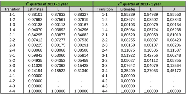
21 Table 10 and table 11 below present the results of the simulation of one year estimated transitions probabilities for the periods of 2008 and 2013:
Table 10 – 1 year estimated transition probabilities for the periods of 2008
Source: the author.
Table 11 – 1 year estimated transition probabilities for the periods of 2013
Source: the author.
Based on the results presented above we can conclude the following:
• Contracts for the period of 2008 - The 1 year estimated transition probabilities can be considered to reflect the state of the contracts in one year and show that contracts stay in state 1 with 70% of probability, and have a probability of about 20% of passing on to state 2. In turn, the probabilities of transition from state 1 to states 3 and 4 are minimal. Analysing state 2, we verify instead that contracts will assume this state with approximately 25% of probability. The results also show that it is more likely a contract will change to a recovery situation (about 50% of probability) than move to a restructuring or default situation (9% and 14% of probability, respectively). As to contracts in stage 3, we conclude that these will maintain their status with
Transition Estimates L U 1-1 0,71327 0,71191 0,71450 1-2 0,21478 0,21374 0,21590 1-3 0,02844 0,02802 0,02888 1-4 0,04351 0,04297 0,04412 2-1 0,51059 0,50866 0,51249 2-2 0,26308 0,26142 0,26471 2-3 0,08746 0,08618 0,08879 2-4 0,13887 0,13737 0,14068 3-1 0,15810 0,15555 0,16082 3-2 0,03057 0,03005 0,03113 3-3 0,74472 0,74124 0,74826 3-4 0,06661 0,06468 0,06860 4-1 0,00000 - -4-2 0,00000 - -4-3 0,00000 - -4-4 1,00000 1,00000 1,00000 1st quarter of 2008 - 1 year Transition Estimates L U 1-1 0,72896 0,72763 0,73042 1-2 0,20164 0,20045 0,20268 1-3 0,02811 0,02766 0,02854 1-4 0,04129 0,04066 0,04188 2-1 0,53500 0,53308 0,53715 2-2 0,24406 0,24245 0,24555 2-3 0,08759 0,08624 0,08897 2-4 0,13334 0,13157 0,13507 3-1 0,16542 0,16253 0,16812 3-2 0,02996 0,02942 0,03048 3-3 0,74149 0,73803 0,74535 3-4 0,06313 0,06113 0,06503 4-1 0,00000 - -4-2 0,00000 - -4-3 0,00000 - -4-4 1,00000 1,00000 1,00000 2nd quarter of 2008 - 1 year Transition Estimates L U 1-1 0,88101 0,87832 0,88327 1-2 0,07692 0,07561 0,07819 1-3 0,00138 0,00113 0,00167 1-4 0,04070 0,03892 0,04296 2-1 0,84295 0,83877 0,84682 2-2 0,07412 0,07277 0,07538 2-3 0,00225 0,00175 0,00291 2-4 0,08068 0,08068 0,08508 3-1 0,59842 0,53060 0,65814 3-2 0,04935 0,04352 0,05459 3-3 0,11029 0,07362 0,15428 3-4 0,24194 0,18522 0,31340 4-1 0,00000 - -4-2 0,00000 - -4-3 0,00000 - -4-4 1,00000 1,00000 1,00000 1st quarter of 2013 - 1 year Transition Estimates L U 1-1 0,85239 0,84939 0,85550 1-2 0,08674 0,08502 0,08843 1-3 0,00103 0,00079 0,00134 1-4 0,05984 0,05724 0,06238 2-1 0,80520 0,80059 0,81019 2-2 0,08255 0,08087 0,08423 2-3 0,00150 0,00107 0,00206 2-4 0,11075 0,10585 0,11587 3-1 0,51922 0,42756 0,60248 3-2 0,05027 0,04112 0,05855 3-3 0,07642 0,04079 0,12564 3-4 0,35409 0,27053 0,45172 4-1 0,00000 - -4-2 0,00000 - -4-3 0,00000 - -4-4 1,00000 1,00000 1,00000 2nd quarter of 2013 - 1 year
22 74% of probability, and consequently there is a 16% probability of recovery. Results also allow for a conclusions that default situations are minimal (6% of probability).
• Contracts for the period of 2013 - In 2013 we can see a significant change in state 2, given that there is a high probability of recovery when a contract is in a non performing situation (around 85%). A change is also observed in state 3. In this case, higher transition probabilities are observed for the recovery state (between 52% and 60%), although the probabilities of transition to default also increased when comparing to 2008.
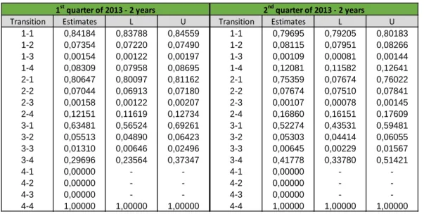
The same simulation was performed by considering instead the state of contracts in 2 years, and results are shown below in table 12 and in table 13:
Table 12 – 2 year estimated transition probabilities for the periods of 2008
Source: the author.
Table 13 – 2 year estimated transition probabilities for the periods of 2013
Source: the author.
Transition Estimates L U 1-1 0,62292 0,62116 0,62489 1-2 0,21057 0,20941 0,21172 1-3 0,06025 0,05935 0,06120 1-4 0,10626 0,10484 0,10754 2-1 0,51235 0,51014 0,51470 2-2 0,18155 0,18036 0,18277 2-3 0,10267 0,10117 0,10434 2-4 0,20344 0,20090 0,20571 3-1 0,24612 0,24259 0,24968 3-2 0,06477 0,06382 0,06579 3-3 0,56178 0,55641 0,56655 3-4 0,12733 0,12409 0,13082 4-1 0,00000 - -4-2 0,00000 - -4-3 0,00000 - -4-4 1,00000 1,00000 1,00000 1st quarter of 2008 - 2 years Transition Estimates L U 1-1 0,64391 0,64314 0,64584 1-2 0,19704 0,19590 0,18250 1-3 0,05899 0,05807 0,05989 1-4 0,10005 0,09854 0,10134 2-1 0,53506 0,53272 0,53748 2-2 0,17007 0,16889 0,17137 2-3 0,10136 0,09977 0,10301 2-4 0,19351 0,19089 0,19584 3-1 0,25927 0,25539 0,26290 3-2 0,06288 0,06179 0,06386 3-3 0,55708 0,55189 0,56271 3-4 0,12077 0,11735 0,12423 4-1 0,00000 - -4-2 0,00000 - -4-3 0,00000 - -4-4 1,00000 1,00000 1,00000 2nd quarter of 2008 - 2 years Transition Estimates L U 1-1 0,84184 0,83788 0,84559 1-2 0,07354 0,07220 0,07490 1-3 0,00154 0,00122 0,00197 1-4 0,08309 0,07958 0,08695 2-1 0,80647 0,80097 0,81162 2-2 0,07044 0,06913 0,07180 2-3 0,00158 0,00122 0,00207 2-4 0,12151 0,11619 0,12734 3-1 0,63481 0,56524 0,69261 3-2 0,05513 0,04890 0,06423 3-3 0,01310 0,00646 0,02496 3-4 0,29696 0,23564 0,37347 4-1 0,00000 - -4-2 0,00000 - -4-3 0,00000 - -4-4 1,00000 1,00000 1,00000 1st quarter of 2013 - 2 years Transition Estimates L U 1-1 0,79695 0,79205 0,80183 1-2 0,08115 0,07951 0,08266 1-3 0,00109 0,00081 0,00144 1-4 0,12081 0,11582 0,12641 2-1 0,75359 0,07674 0,76022 2-2 0,07674 0,07510 0,07841 2-3 0,00107 0,00078 0,00145 2-4 0,16860 0,16151 0,17609 3-1 0,52274 0,43531 0,59481 3-2 0,05303 0,04414 0,06055 3-3 0,00645 0,00229 0,01567 3-4 0,41778 0,33780 0,51421 4-1 0,00000 - -4-2 0,00000 - -4-3 0,00000 - -4-4 1,00000 1,00000 1,00000 2nd quarter of 2013 - 2 years
23 Based on the results of this analysis we can conclude the following:
• Contracts for the period of 2008 – There is a lower probability for contracts in state 1 to remain in this state (62% and 64%) and the probability of default increases from 4% to 10%. As to state 2, we can see that contracts will maintain their status with a probability of 18% (lower when comparing with 2013 and the probability of default rises to 20%. In state 3 there is 56% of probability that contracts will maintain in this state and the probability of transition to state 1 is higher when compared with the default state (26% and 13%, respectively).
• Contracts for the period of 2013 – These contracts present higher probabilities of recovery when we analyse the non performing and restructuring states. In the first situation, the probabilities increase, at least, 20%. The restructured contracts present between 52% and 63% of recovery, which is considerably higher when comparing to the figures of 2008. Although there is a good recovery perspective for the restructuring event, one also has to consider that the transition to the state of default presents a significant risk when comparing with the case in 2008, given that the probabilities increase from 13% (in 2008) to a maximum of 41% (2013).
To briefly summarize, for the year of 2008 one can conclude that contracts in states 1 and 3 will maintain their position with a high probability. Results also show that non performing and restructured contracts are more suitable to a recovery scenario than the default. Regarding the 2013 data, we observe that contracts in state 1 will maintain their position with an even higher probability (when comparing with results for 2008). In turn, contracts in state 3 have a significantly different behavior, give that they not only present higher probabilities of recovery but also higher probabilities associated to the default status. The probability of remaining in this state is considerably lower (again, when comparing with 2008) but this can be explained in part by the short historical period of these contracts. Overall, the behavior for the contracts of 2013 is less risky when compared with that observed for the 2008 dataset.
The latest observation point for the contracts used in this work is June 2015. Based on the assumption that contracts that reach this point are still active in Fannie Mae portfolios, it is important to study and predict the behaviour of these contracts regarding their future status. Therefore, the following analysis relies on the observation of the number of contracts by each state, in June 2015, and the application of the estimated transition probabilities in order to predict the number of contracts in each state in June 2016 and June 2017.
Table 14 – Number of active contracts observed in June 2015
Source: the author.
2008_Q1 2008_Q2 2013_Q1 2013_Q2
State 1 19.367 18.936 12.285 10.372
24
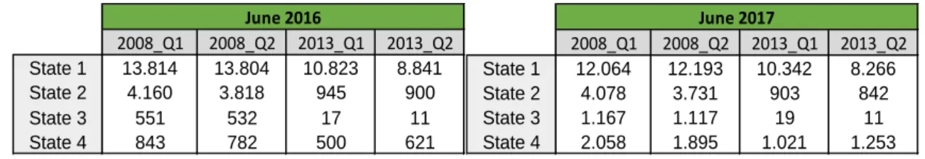
Table 15 – Estimated number of contracts in each state in June 2016 and June 2017 for the portfolios of 2008-13
Source: the author.
Table 14 above illustrates the number of contracts in each portfolio under analysis and their status in June 2015. Since that are only observed contracts in states 1 and 4 in this date, it is only possible to estimate transitions from state 1 (state 4 is ignored given the fact that this state is the absorbent state). Table 15 shows the results regarding the expected number of contracts in each state in June 2016 and June 2017, given by the product between the estimated transition probabilities within 1 and 2 years and the number of contracts by state in June 2015. Results show that the predominant state in terms of number of contracts is state 1, while state 3 appears to be the least represented. Taking in consideration portfolios of 2008, results also show that the number of contracts in state 1 decreases between 2016 and 2017, while the number of contracts in states 3 and 4 duplicates. The same conclusion can be drawn for the portfolios of 2013 regarding states 1 and 4. Finally, we also conclude that contracts tend to be in higher risk states the longer the forecast time.
2008_Q1 2008_Q2 2013_Q1 2013_Q2 State 1 13.814 13.804 10.823 8.841 State 2 4.160 3.818 945 900 State 3 551 532 17 11 State 4 843 782 500 621 June 2016 2008_Q1 2008_Q2 2013_Q1 2013_Q2 State 1 12.064 12.193 10.342 8.266 State 2 4.078 3.731 903 842 State 3 1.167 1.117 19 11 State 4 2.058 1.895 1.021 1.253 June 2017
25
5. CONCLUSION
The work at hand consisted on an application of a multi-state Markov model in continuous time to mortgage loans in order to predict the behaviour of clients who have not complied with their credit obligations. With this analysis, it was possible to summarize the progression of the loans, namely their movements of recovery, restructuring or default. Given the results illustrated previously, for 2008 there is evidence that the risk associated to the possible transitions is not significant, since there were little to no changes in the contracts’ state during the month’s progression. Comparing to 2013, the estimation of the transition intensity matrices shows that the possibility of a recovery scenario is quite stronger than a default scenario for the observed loans.
Through the estimation of intensity matrices for 2008 and 2013 several models could be obtained, indicating the transition probabilities in a chosen time horizon, with the use (or not) of different covariates. Overall, these estimates showed that contracts have high probabilities of remaining in states 1 and 3, that a recovery scenario is more likely than a default scenario, and that the 2008 portfolio is riskier. The application of the estimated probabilities to the observed active contracts also provided significant information regarding the future number of contracts in each state for the portfolios under analysis.
In addition, to providing important results that allow for a better understanding of the contracts behaviour, the multi-state Markov model also allowed us to estimate the mean sojourn times in each transient state, therefore providing a powerful contribute in terms of time prediction of the possible transitions.
According with the number of contracts held by Fannie May we noted that, although the crisis of 2008 lead the company to a state of conservatorship, it continued to grow in terms of number of loans acquired. Based on the observed numbers of 2013, the number of contracts with days past due are significantly less than the number observed in 2008, which can lead one to conclude that the company took a preventive strategy regarding the type of contracts that it acquires/maintains in its portfolio.
Throughout the analysis performed in this work several limitations arose, mainly due to the size of the available data. Fannie Mae provides the information about their loans in quarterly groups and in each one of these groups there is information for each contract. One contract only appears in one quarter and based on this, to perform a multi-state model for one year it was necessary to group four groups of information. Taking into consideration the amount of information, it was challenging for R software to perform any kind of model, which is why this study was performed on a quarterly basis. Based on this approach, results showed that the first and second quarters of 2008 present similar patters to the third and fourth quarters (the same was observed for 2013); therefore to prevent repetitive conclusions, only the first two quarters of each year were considered in this study.
Despite the identified limitations, it is considered that the study carried out allowed us to understand contracts’ movement as well as the time associated to these transitions, being an important contribute to predict the behaviour of clients who have not complied with their credit obligations. A study considering covariates, in order to study the relation of constant or time-varying characteristics of individuals with their transition rates, would be a good approach in the development of studies using multi-state Markov models in the credit risk modelling.
26
6. BIBLIOGRAPHY
Altman, E. I. (1968). Financial Ratios, Discriminant Analysis and the Prediction of Corporate Bankruptcy. The Journal of Finance, 23(4): 589–609.
Altman, E.I. and Narayanan, P. (1997). An International Survey of Business Failure Classification Models. Financial Markets, Institutions and Instruments, 6(2): 1–57.
Andersen, P.K., Borgan, O., Gill, R.D. and Keiding, N. (1993). Statistical Models Based on Counting
Processes. Springer, New York.
Andersen, P. K., and Keiding, N. (2002). Multi-state models for event history analysis. Statistical
methods in medical research, 11(2): 91–115.
Bharath, S. and Shumway, T. (2008). Forecasting Default with the KMV-Merton Model. The Review of
Financial Studies, Volume 21, Issue 3, 1 May 2008, Pages 1339–1369.
Black, F. and Cox, J. (1976). Valuing Corporate Securities: Some Effects of Bond Indenture Provisions.
The Journal of Finance, 31(2): 351-367.
Chamboko, R. and Bravo, J. M. (2016). On the Modelling of Prognosis from Delinquency to Normal Performance on Retail Consumer Loans. Risk Management, 18(4): 264–287.
Chen, W., Xiang, G., Liu, Y., and Wang, K. (2012). Credit risk Evaluation by hybrid data mining technique. Systems Engineering Procedia 3: 194–200.
Cox, D. R. and Miller, H. D. (1965). The Theory of Stochastic Processes. Chapman and Hall, London. Credit Suisse First Boston International (1997). Creditrisk+: A Credit Risk Management Framework. Technical Report (London: Credit Suisse First Boston). Available via the Internet: http://www.csfb.com/institutional/research/assets/creditrisk.pdf
Demyanyk, Y. and Van Hemert, O (2011). Understanding the Subprime Mortgage Crisis. Review of
Financial Studies, 24(6): 1848–1880.
Duffie, D. and Lando, D. (2000). Term Structure of Credit Spreads With Incomplete Accounting Information, Econometrica, 60(3): 633–664.
Federal Housing Finance Agency (2018). About FHFA. Retrieved 28 February 2018, from Http://www.fhfa.gov/AboutUs.
Federal Housing Finance Agency (2018). Conservatorship. Retrieved 28 February 2018, from Http://www.fhfa.gov/Conservatorship.
Fannie Mae (2018). Fannie Mae Single-Family Loan Performance Data. Retrieved 28 February 2018, from Http://www.fanniemae.com/portal/funding-the-market/data/loan-performance-data.html. Geske, R. (1977). The Valuation of Corporate Liabilities as Compound Options. Journal of Financial
27 Hull, J. and White, A. (1995). The Impact of Default Risk on the Prices of Options and Other Derivative Securities. Journal of Banking and Finance, 19(2): 299–322.
Imielinski, T and Mannila, H (1996). A database perspective on knowledge discovery.
Communications of the ACM. 39(11): 58–64.
Jackson, C. H. (2011). Multi-state Models for Panel Data: The msm Package for R. Journal of Statistical
Software, 38(8): 1–26.
Gupton, G. M., Finger, C. C. and Bhatia M. (1997). Credit Metrics: Technical Document, J.P. Morgan & Co., New York.
Jones, E., Mason, S. and Rosenfeld, E. (1984). Contingent Claims Analysis of Corporate Capital Structures: An Empirical Investigation. Journal of Finance, 39(3): 611–627.
Kalbfleisch, J. D. and Lawless, J. F. (1985). The analysis of panel data under a Markov assumption.
Journal of the American Statistical Association, 80(392): 863–871.
Kay, R. (1986). A Markov model for analysing cancer markers and disease states in survival studies.
Biometrics, 42(4): 855–865.
Kim, J., Ramaswamy, K. and Sundaresan, S. (1993). Does Default Risk in Coupons Affect the Valuation of Corporate Bonds? A Contingent Claims Model. Financial Management, 22(3): 117–131.
Kleinbaum, D. G. and Klein, M. (2012). Survival Analysis: A Self-Learning Text. 3rd Edition, Springer, New York.
Lo, A. (1986). Logit versus discriminant analysis: A specification test and application to corporate bankruptcies. Journal of Econometrics, 31(2): 151–178.
Longstaff, F. and Schwartz, E. (1995). A Simple Approach to Valuing Risky Fixed and Floating Rate Debt. Journal of Finance, 50(3): 789–819.
Malik, M. and Thomas, L. C. (2012). Transition matrix models of consumer credit ratings. International Journal of Forecasting, 28(1): 261–272.
Martin, D. (1977). Early warning of bank failure: A logit regression approach. Journal of Banking &
Finance, 1(3): 249–276.
Merton, R. C. (1974). On the Pricing of Corporate Debt: the Risk Structure of Interest Rates. The
Journal of Finance, 29(2): 449-470.
Ohlson, J. (1980). Financial ratios and the probabilistic prediction of bankruptcy. Journal of
Accounting Research, 18(1): 109–131.
Russell, S. and Norvig, P. (2010). Artificial Intelligence: A Modern Approach (Third Edition), Pearson, New York.
So, M.C. and Thomas, L.C. (2010) Modelling and model validation of the impact of the economy on the credit risk of credit card portfolios. Journal of Risk Model Validation, 4(4): 93–126.
28 Trench, M. S., Pederson, S. P., Lau, E. T., Ma, L., Wang, H., and Nair, S. K. (2003). Managing credit lines and prices for Bank One credit cards. Interfaces, 33(5): 4–21.
Vasicek, O. (1984). Credit Valuation. Journal of Financial Risk Management, 3(2). Wilson, T. (1998). Portfolio Credit Risk. Economic Policy Review, 4(3): 71–82.