School of Social Sciences Department of Political Economy
Determinants of the Portuguese Government Bonds Yields
André Miguel dos Santos Castro Pinho
Dissertation submitted as partial requirement for the conferral of
Master in Monetary and Financial Economics
Supervisor:
Doctor Ricardo Barradas Invited Assistant Professor, Polytechnic Institute of Lisbon
I
School of Social Sciences Department of Political Economy
Determinants of the Portuguese Government Bonds Yields
André Miguel dos Santos Castro Pinho
Dissertation submitted as partial requirement for the conferral of
Master in Monetary and Financial Economics
Supervisor:
Doctor Ricardo Barradas Invited Assistant Professor, Polytechnic Institute of Lisbon
III
Acknowledgments
I am extremely grateful to Professor Ricardo Barradas for all his availability, dedication and mostly for the knowledge transmitted during the elaboration of this dissertation.
I also want to express a huge gratitude to my family, for all the guidance and support during all these years and for the motivation to proceed with this work.
Finally, I also want to express my enormous gratitude to Caixa Económica Montepio Geral as well as to those who work with me everyday.
V Resumo
Esta dissertação faz uma análise empírica à evolução das yields da divida pública portuguesa, procurando identificar os seus principais determinantes, para o período entre 2000 e 2016 usando dados trimestrais. Foi estimada uma equação para as yields da divida pública portuguesa considerando três maturidades distintas (um, cinco e dez anos) e incluindo oito variáveis independentes (PIB, divida pública, divida externa, produtividade do trabalho, taxa de atividade, taxa de inflação, volatilidade do mercado acionista e liquidez) de modo a capturar de forma global os efeitos do risco de crédito, da aversão global ao risco bem como do risco de liquidez. Os resultados demonstraram que o PIB, a divida externa, a taxa de inflação e a liquidez influenciam positivamente as yields da divida pública com maturidade a dez anos enquanto que a divida pública, a produtividade do trabalho, a taxa de atividade e a volatilidade do mercado acionista afetam negativamente as yields. Foram ainda encontradas evidências que apoiam o sinal contraditório ao que a maioria da literatura afirma relativamente à divida pública. No GERAL, os resultados apontam que não existem grandes diferenças nos determinantes para as diferentes maturidades. Finalmente, concluímos que a liquidez, a produtividade do trabalho, mas sobretudo a divida externa foram os fatores que originaram uma subida das yields, enquanto que a taxa de atividade, o PIB, a divida pública e a inflação revelaram ter um efeito benéfico sobre as yields da divida pública portuguesa.
Palavras-chave: Portugal, Yields da divida pública, Cointegração, Modelos ARDL, Determinantes de longo e curto prazo
VII Abstract
This paper makes an empirical analysis of the evolution of Portuguese government bonds yields in order to identify their main determinants for the period between 2000 and 2016 using quarterly data. An equation of the Portuguese government bonds yields is estimated considering three different maturities (one, five and ten years) and including eight independent variables (GDP, public debt, external debt, labour productivity, activity rate, inflation rate, stock market volatility and liquidity) to capture the global effects of credit risk, global risk aversion and the liquidity risk. Our main findings were that GDP growth rate, external debt, inflation rate and liquidity exert a positive effect on the ten year maturity sovereign bond yields while public debt, labour productivity, activity rate and the stock market volatility affect negatively the yields. Evidence supporting the contradictory sign of what the majority of the literature claims regarding public debt is also found. Overall, the results point out that there are no significant differences regarding the determinants of the government bonds yields for the different maturities. Finally, we conclude that the yields were harmful affected by liquidity, labour productivity but mostly by external debt. In turn, activity rate, GDP, public debt and mostly the inflation rate had a beneficial effect on the Portuguese government bonds yields.
Keywords: Portugal, Sovereign bond yields, Cointegration, ARDL Models, Long-run and short-run determinants
IX Table of Contents
List of Figures ... XI
List of Tables ... XIII
I. Introduction ... 1
II. Literature review ... 3
III. Model and Hypothesis ... 9
IV. Data ... 13
V. Methodology ... 17
VI. Results and Discussion ... 21
VII. Conclusion ... 32
VIII. References ... 34
XI List of Figures
Figure 1 -- Government bonds yields risk drivers... 3
Figure 2 - Portuguese ten-year maturity sovereign bond yields ... 36
Figure 3 - Portuguese five-year maturity sovereign bond yields ... 36
Figure 4 - Portuguese one-year maturity sovereign bond yields ... 37
Figure 5 - GDP growth rate (annual rate of change) ... 37
Figure 6 - Public debt (% of GDP) ... 38
Figure 7 - External debt (% of GDP) ... 38
Figure 8 - Labour productivity (annual rate of change) ... 39
Figure 9 - Activity rate ... 39
Figure 10 - Inflation rate (annual rate of change) ... 40
Figure 11 - Implied stock market volatility index (VIX) ... 40
Figure 12 - Portuguese government bonds liquidity ... 41
Figure 13 - The ten-year maturity sovereign bond yields plot of cumulative sum of recursive residuals ... 42
Figure 14 - The ten-year maturity sovereign bond yields plot of cumulative sum of squares of recursive residuals ... 42
Figure 15 - The five-year maturity sovereign bond yields plot of cumulative sum of recursive residuals ... 43
Figure 16 - The five-year maturity sovereign bond yields plot of cumulative sum of squares of recursive residuals ... 43
Figure 17 - The one-year maturity sovereign bond yields plot of cumulative sum of recursive residuals ... 44
Figure 18 - The one-year maturity sovereign bond yields plot of cumulative sum of squares of recursive residuals ... 44
XIII List of Tables
Table 1 - The correlation matrix between variables ... 14
Table 2 - P-values of the ADF unit root test ... 15
Table 3 - P-values of the PP unit root test ... 16
Table 4 - Values of information criteria ... 21
Table 5 - Bounds test for cointegration analysis (short version) ... 22
Table 6 - Diagnostic tests for ARDL estimations ... 22
Table 7 - Long-term estimations of sovereign bond yields ... 24
Table 8 - Short-term estimations of the ten year maturity government bond yields ... 26
Table 9 - Short-term estimations of the five year maturity government bond yields ... 26
Table 10 - Short-term estimations of the one year maturity government bond yields ... 27
Table 11 - Economic significance of our estimates for Portuguese government bond yields by maturity ... 27
1
I. Introduction
It is known that countries borrowing costs have a large impact on their policies and budgetary decisions, which raises a great deal of interest in perceiving the factors that affect those costs. There is also a significant interest by private investors holding fixed income public debt securities, since the anticipation of future movements in the yields have an impact on the prices and therefore may originate profits or losses on their investment portfolios.
There are several factors that may influence positively, negatively or causing an ambiguous effect on sovereign bond yields. The usually ones are macroeconomic performance, fiscal conditions, inflation rate, global risk aversion and liquidity. Foreign borrowing, labour productivity and demographics are also factors that may influence sovereign funding costs.
Since most of the studies are panel data based and there are no studies related to Portugal, at least to our knowledge, the objective of this work is to complement the existing literature by exploring in particular which variables explain the Portuguese sovereign bonds yields as well as to measure the exact magnitude of the impacts. It is also worth noting that the yields spread between Portuguese and German sovereign bonds increased significantly since the first quarter of 2008 onwards, which in turn strengthens and motivates the search for the concrete factors that led to the increase of Portuguese government funding costs.
Thus, this study aims to explore the main determinants of the Portuguese sovereign bonds yields besides the traditional factors that are usually considered - i) current and expected central bank interest rates and ii) the country default risk.
The analysis considers the long, medium and short-term sovereign bonds yields and covers the period from 2000 to 2016. In this way, three equations are estimated using eight independent variables (GDP growth rate, public debt, external debt, labour productivity, activity rate, inflation rate, stock market volatility and liquidity). Since our variables are integrated of order zero and one, the outputs are produced using the ARDL estimation technique.
Our main findings relative to the long run are that GDP growth rate, external debt, inflation rate and liquidity are positive determinants of the yields while the public debt, labour productivity, activity rate and the stock market volatility are negative determinants. Moreover, public debt presents a contradictory sign to what the majority of literature claims since an increase on public
2
debt lowers the government bond yields. Additionally, some variables stopped being statistically relevant as the yields maturities decrease.
In general, the main results point out that there were no significant differences regarding the long-term determinants of the government bonds yields among the different maturities considered.
Furthermore, we also conclude that the yields were harmful affected by liquidity, labour productivity and by external debt, with the latter one having the major impact. On the other hand, the activity rate, GDP, the public debt and mostly the inflation rate proved to have a beneficial effect, except for the Crisis and Post-Crisis period, in which inflation rate had a contradictory effect as its increase led to a rise on the Portuguese government bonds yields.
This dissertation is organized as follows: Chapter 2 covers the related literature, Chapter 3 presents the economic model and hypothesis, Chapter 4 covers the data and explains the construction of the variables, Chapter 5 explains the methodology, Chapter 6 presents the empirical results and Chapter 7 summarizes the conclusions.
3
II. Literature review
In order to perform our study, we need to know the main determinants of government bond yields identified by the literature on this matter.
The existing studies on this subject, that typically fall into two categories: single-country and panel data studies, modelled the government bond yields considering three main risk drivers, which we summarize in the figure below (Figure 1, Afonso et. al., 2015).
Figure 1 -- Government bonds yields risk drivers
Government Bonds Yields
Macroeconomic performance Fiscal conditions
Credit risk Inflation
Foreign borrowing Labour productivity Demographics
Global risk aversion
Liquidity risk
Source: Authors’ representation based on Afonso et. al. (2015), among others
According to the majority of these studies, the credit risk of a certain country reflects the macroeconomic performance and fiscal conditions. The variable used for modelling macroeconomic performance that appears to be more significant in the literature is either the potential GDP growth (Poghosyan, 2014; Pham, 2014) or the GDP growth rate (Baldacci and Kumar, 2010; Hsing, 2015).
The linkage between potential GDP growth and government bond yields can be explained, according to Laubach (2009), using the Ramsey model of optimal growth. Combined with a representative household with CES utility, the Ramsey model implies that the real rate of return on capital (i.e., real interest rate) is determined by:
where r is the rate of return, g denotes the net growth rate of technology, output and consumption, 𝜎 is the coefficient of relative risk aversion and 𝜃 is the household’s rate of time
4
preference. Thus, the rate of return depends positively on those three parameters, namely GDP growth rate.
In addition, Poghosyan (2014) suggests that short run positive deviations of output growth from its potential level may reduce sovereign borrowing costs as the country temporary taxing capacity increases. This rational shall apply to negative deviations of output growth once the country taxing capacity decreases, which in turn may cause a rise on governments borrowing costs.
As about fiscal conditions, Government debt and Primary balances (Baldacci and Kumar, 2010; Ichiue, 2012; Pham, 2014; Poghosyan, 2014) or even Budget and Current account balances (Afonso and Rault, 2010) are the variables that more often appear as determinants in the literature. The literature presents two channels of impact through which fiscal conditions may influence long-term interest rates: crowding out effect and default risk premium. Through the first channel of impact, according to Engen and Hubbard (2005), private investment may be crowded out by fiscal expansion, which results in a lower steady-state capital stock, leading to a higher marginal product of capital and thus an increase on interest rates. According to the second channel of impact, the deterioration of fiscal conditions leads to a higher probability of default and consequently a demand by investors for a higher risk premium, which in turn rises sovereign borrowing costs (Baldacci and Kumar, 2010).
Also regarding fiscal conditions, the literature presents some interesting conclusions. First, some studies tend to use expected fiscal deficits rather than past or current deficits in order to measure the impact on long-term government bond yields (Haugh et al., 2009; Ichiue, 2012). This can be well understood since future fiscal developments matters more regarding investment decisions than past outcomes. Second, the impact of the level of public debt turns out to be quantitatively lower than the one of public deficits, which contradicts the theoretical idea that stock fiscal variables (i.e., public debt) influence long term interest rates but flow fiscal variables (i.e., fiscal deficits) do not (Engen and Hubbard, 2005).
As about the latter conclusion, despite the majority of studies conclude that fiscal imbalances tend to raise long term sovereign bond yields, the impact range from 2 to 5 basis points for each 100 basis points increase considering stock fiscal variables such as debt-to-GDP ratio (Ardagna
et. al., 2007; Poghosyan, 2014) and from 10 to 25 basis points if flow fiscal variables such as
5
fact, if flow variables reveal to be persistent over time, they may provide useful information for forecasting future stock variables (Ichiue, 2012).
Moreover, Ardagna et al. (2007), using a panel of 16 OECD countries and historical data from 1960 to 2002, conclude that the effects on interest rates are greater as a country’s debt grows and its fiscal balance becomes weaker. In addition, Baldacci and Kumar (2010), also conclude that higher deficits and levels of public debt lead to a significant increase in long term interest rates and that the magnitude of such impacts reflects the initial fiscal condition as well as institutional and structural condition, but also spillovers from global financial markets.
More recently, Dell’Erba and Sola (2011), using a sample of 17 OECD countries, point out that common fiscal shocks lead to adjustments in the European sovereign bond yields, having a greater impact in smaller and peripheral countries. This may suggest, in events of this nature, that bond owners tend to rearrange their investment portfolios, by selling their debt securities issued by those countries and reinvest on sovereign bonds of countries with stronger economies and better fiscal conditions.
The third factor that is pointed out as being a determinant of the government bond yields is the inflation rate – either through historical rates (Ardagna et. al., 2007; Poghosyan, 2014) or expected rates (Hsing, 2015). In this way, related literature suggest it may influence nominal interest rates through two channels of impact: the level of inflation rate itself and the uncertainty that is normally associated with it.
Accordingly, Baldacci and Kumar (2010) suggest that higher inflation expectations may push upwards sovereign bond yields, through the increase of inflation premium embodied in nominal rates, especially in times where output deviations are positive or there are concerns about monetization of debt. Moreover, according to Baldacci et. al. (2008), inflation expectations could also generate macroeconomic uncertainty leading to higher country risk premium and therefore a rise on sovereign bond yields. More recently, Hsing (2015), through his single-country analysis to Spain over the period 1999 to 2014, concludes that an increase in the expected inflation rate contributes to an increase on sovereign funding costs.
Regarding foreign borrowing, the variable used for modelling that appears to be more often stated is the level of external debt (Cantor and Packer, 1996; Ichiue, 2012). In this way, Ichiue (2012) also suggest that when an increase in the government debt is financed entirely by borrowing from external sources, the increase on the interest rate is approximately twice than if it was financed by domestic savings. The argument given by the authors is that the losses
6
tend to be greater when the government depends more on domestic investors - therefore there is a strong incentive in choosing to increase the national tax revenues instead of defaulting.
As about the latter two factors that may have impact on credit risk (labour productivity and demographics), they seem to have not been much explored in the sovereign bond yields related literature. Effectively, these two specific variables are less common in empirical studies on determinants of government bonds yields.
However and regarding labour productivity, Ichiue (2012), by employing a forecast of the annualized labour productivity growth rate, conclude that an increase in the expected productivity growth rate leads to a rise in the long-term interest rates in a similar extent. In fact, a higher labour productivity enables the firms to afford higher wages, which in turn contributes to a higher inflation therefore an increase on risk premiums demanded by market participants.
As about demographics, the literature presents contradictory effects on long-term interest rates. On the one hand, it is often argued that population ageing lowers the marginal productivity of capital and reduces investment demand through a decrease in the labor supply which in turn contributes to a downward pressure on long-term interest rates. On the other hand, some claims that ageing can contribute to an increase of interest rates through the life cycle hypothesis, in which individuals begin to spend their savings after retirement, which leads to a decrease in the savings rate. In relation to the first argument, Ichiue (2012) conclude on the existence of a strong positive relationship, suggesting that a decline in the working-age population ratio is associated with population ageing, which exert a negative effect on the long-term interest rates.
The second sovereign bond yields risk driver is the global risk aversion, which has the objective of capturing the level of investors perceived financial risk as well as their sentiment towards the bond securities market. According to the majority of the empirical analysis, this factor is either empirically approximated using corporate bonds spreads (Haugh et al., 2009) or stock market implied volatility indexes (Afonso et. al., 2015) and proved to have a stronger effect mainly during periods of tightening financial conditions (Haugh et al., 2009).
Finally, the liquidity risk refers to the size and depth of the government bonds market and captures the possibility of capital losses due to significant price reductions resulting from a small number of transactions in the market. Most of the studies tend to use either government bonds bid-ask spreads (Afonso et. al., 2015) or the share of a country’s government debt on global Economic and Monetary Union (EMU) sovereign debt in the case of the euro area countries. According to the literature, some claim that liquidity tends to vary inversely with the
7
size of the market, as for large bond markets investors can trade quickly and face a lower risk that prices will significantly change therefore they demand less compensation in terms of the yield (Haugh et al., 2009). Moreover, liquidity effects are found to be greater during periods of tightening financial conditions and higher interest rates, during which the market players accept to trade lower yields for higher government debt liquidity (Favero et. al., 2010).
To conclude, the literature review provides empirical support on the theoretical prediction that variables linked with credit risk as well as global risk aversion and liquidity risk, have an impact on sovereign bond yields. Since most of the studies are panel data based and there are no studies related to Portugal, at least to our knowledge, our objective is to extend the existing literature by exploring in particular which variables explain the Portuguese government bonds yields as well as to measure the exact magnitude of the impacts.
9
III. Model and Hypothesis
We estimate an equation where the Portuguese government bonds yields becomes a function of eight variables: GDP growth rate, public debt, external debt, labour productivity, activity rate, inflation rate, stock market volatility and liquidity.
Accordingly, our long-term equations take the following form:
, where PT10Y, PT5Y and PT1Y are the ten, five and one year maturities government bond yields respectively, GDP is the gross domestic product growth rate, PD is the public debt, ED is the level of external debt, LP is the labour productivity, AR becomes the activity rate, INF is the inflation rate, VIX is the stock market volatility and L is the liquidity. Moreover, μt is an independent and identically distributed (white noise) disturbance term with null average and constant variance.
Regarding the effect of each variable on government bonds yields, the GDP growth rate, public debt, external debt and inflation rate are expected to impact positively while stock market volatility is expected to impact the yields negatively. In turn, labour productivity, activity rate and liquidity may either have a positive or a negative impact on the yields.
Thus, the coefficients of those variables are expected to have the following signs:
𝛽1 > 0, 𝛽2 > 0, 𝛽3 > 0, 𝛽4 ≷ 0, 𝛽5 ≷ 0, 𝛽6 > 0, 𝛽7 < 0, 𝛽8 ≷ 0 (2) (3) (4) (5)
10
As about the first one, according to the Ramsey model of optimal growth (explained in the section above), GDP growth rate affects the yields in a positive way, therefore we expect the coefficient to have a positive sign. However, in the short run, positive deviations of output growth from its potential level may have the contradictory effect. The explanation is that the country has a greater ability to pay for the debt as the temporary taxing capacity rises, which in turn leads to the decrease of sovereign borrowing costs.
The public debt is also expected to affect sovereign bond yields in a positive way through the two channels of impact described in the section above: crowding out effect and default risk premium. The first one tells us that higher levels of public debt may lead private investment to be crowded out by fiscal expansion, which results in a lower steady-state capital stock, leading to a higher marginal product of capital – therefore increasing long-term interest rates (Engen and Hubbard (2005). As about the second channel, greater levels of public indebtedness lead to a higher probability of a country’s default which results in a higher risk premium requested by investors and thus rising government bond yields (Baldacci and Kumar, 2010).
The external debt is also supposed to influence government bond yields in a positive way. The argument is that if a large part of a country’s public debt is being financed from external sources rather than from domestic investors, the government depends less on domestic savings and therefore the incentive to choose to default is higher than rising national tax revenues (Ichiue, 2012). Thus, investors tend to require a higher risk premium, which in turn leads to the increase of sovereign bond yields.
Labour productivity may exert either a positive or a negative influence on sovereign bond yields. On the one hand, an increase on labour productivity makes it possible for firms to afford higher wages, which contributes to a higher inflation rate therefore influencing higher nominal interest rates through an increase of risk premiums. On the other hand, especially during periods of tightening financial conditions, investors might look at an increase of labour productivity as a sign of a strengthening the economy therefore they are willing to accept lower yields as a part of ‘flight-to-quality’ movement.
Regarding the effect of the activity rate on government bond yields, it could impact positively or negatively. For example, population ageing lowers the marginal productivity of capital and reduces investment demand through a decrease in the labour supply, contributing to lower the interest rates. In turn, ageing contributes to increasing long-term interest rates through the life cycle hypothesis, where individuals begin to spend their savings after retirement, therefore a
11
decrease in the savings rate due to population ageing can lead to a rise in long-term sovereign bond yields.
Inflation rate is expected to influence interest rates in a positive way either through the level of the inflation rate itself (Afonso and Rault, 2010) or through the future inflation uncertainty (Ichiue, 2012). Thus, both channels shall influence nominal interest rates through higher risk premiums required by investors if the current or expected inflation turns out to be higher in the future.
The stock market volatility may affect government bond yields in a negative way. The argument behind this is that when the stock market volatility rises, investors tend to rearrange their portfolios investment by moving from stock to the bonds market in order to avoid the volatility. Thus, a higher demand for bonds contributes to increase the bonds prices, which in turn leads to the decrease of the yields.
As about liquidity, the effect is relatively ambiguous since it can impact bond yields in a positive or in a negative way. On the one hand, since it captures the possibility of capital losses due to early liquidation or significant price reductions resulting from a small number of transactions, investors should have to pay an additional premium for bond securities with higher liquidity therefore contributing to an increase on the yields. On the other hand, market participants are willing to trade lower yields for higher sovereign debt liquidity during periods of tightening financial conditions (Favero et. al., 2010).
13
IV. Data
To proceed our study, we have considered the variables using quarterly data between the period from the first quarter of 2000 to and the last quarter of 2016. The historical period and data frequency could not be others since the majority of the variables are only available from 2000 onwards and for some variables such as the GDP growth rate, we did not have historical data with less than quarterly frequency.
In this way, our main dependent variable – ten-year maturity government bond yields (PT10Y) was collected from Bloomberg database. Since available data was on daily frequency, we had to compute the average yield of each quarter. In addition, we have also extracted from Bloomberg the five and one year government bonds yields maturities and the same procedures were applied.
The GDP growth rate (GDP) denotes the variable used to capture macroeconomic performance. In practice, we have computed the year-on-year rate of change from real gross domestic product (at constant prices and in millions of euros), obtained from the Portuguese Nacional Accounts and available at Instituto Nacional de Estatística.
The public debt (PD) represents the proxy used to consider the fiscal conditions factor. It is the total general government gross debt as a percentage of GDP, obtained from Banco de Portugal database.
The net external debt (ED) is used to proxy the effects of foreign borrowing on sovereign funding costs. This variable was extracted from Banco de Portugal database and represents the total net external debt as a percentage of GDP.
The labour productivity (LP) was computed dividing the total employment (in number of individuals) by the gross domestic product at current market prices and then calculated the year-on-year rate of change. Both inputs were collected from the Portuguese National Accounts, available at Instituto Nacional de Estatística.
Activity rate (AR) is used here as the proxy to represent the demographics risk factor. The variable can be described as the total active population divided by total population with ages between 15 and 64. It was extracted from Banco de Portugal database.
14
Inflation rate (INF) is given by the annual rate of change considering as input the global Consumer Price Index – variable available at Instituto Nacional de Estatística database. Since the only frequency available was monthly data, we then had to calculate the average rate of each quarter.
The logarithm of the S&P 500 implied stock market volatility index (VIX index) is the proxy considered for modelling international global risk aversion - variable collected from Bloomberg database. In addition to the extraction, we had to calculate the average value of the index for each quarter, as the available data had daily frequency.
The measure used to gauge the liquidity in the bonds market is the liquidity ratio (L). This variable was computed considering the Portuguese general government consolidated gross debt over the government consolidated gross debt of Euro area countries – both inputs were collected from Eurostat database. This indicator gives an approximation of Portugal’s public debt market share over the global EMU-wide sovereign debt.
Figures 2 to 12 in the Appendix contains the plots of our eleven variables and Table A1 in the Appendix the descriptive statistics of the data. The Table 1 contains the correlation matrix between the variables.
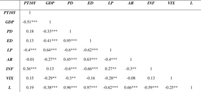
Table 1 - The correlation matrix between variables1
PT10Y GDP PD ED LP AR INF VIX L
PT10Y 1 GDP -0.51*** 1 PD 0.18 -0.33*** 1 ED 0.13 -0.41*** 0.95*** 1 LP -0.4*** 0.64*** -0.6*** -0.62*** 1 AR -0.01 -0.27** 0.45*** 0.63*** -0.4*** 1 INF 0.36*** 0.13 -0.6*** -0.66*** 0.27** -0.3** 1 VIX 0.15 -0.29** -0.3** -0.16 -0.28** -0.08 0.13 1 L 0.19 -0.38*** 0.96*** 0.97*** -0.62*** 0.66*** -0.59*** -0.25** 1
Note: *** indicates statistical significance at 1% level, ** indicates statistical significance at 5% level and * indicates statistical significance at 10% level
1 The correlation coefficients considering the five and one year government bonds yields maturities
15
It is worth noting that most of the coefficients seem to have the correct signs as the variables that present a positive (negative) correlation coefficient are the variables that are expected to affect in a positive (negative) way the ten year maturity sovereign bond yields. On the other hand, GDP and stock market volatility (VIX) present contradictory signs as both variables were supposed to affect the yields in a positive and in a negative way, respectively. In the next section, we will assess this issue by analyzing causality.
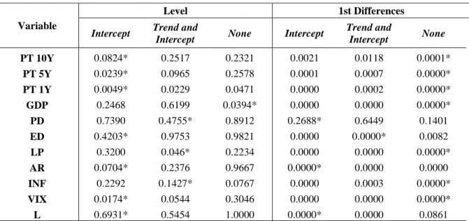
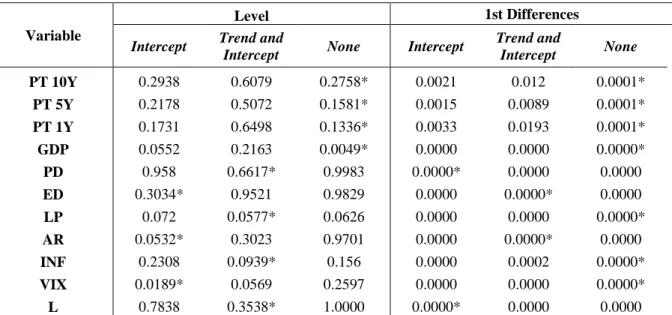
We then checked for the presence of unit roots for each of our eleven variables by performing the Phillips and Perron (1998) and the Augmented Dickey Fuller (1979) unit root tests, which is crucial to the choice of our methodology.
Analyzing the results we concluded that some of the variables were stationary in levels and others were integrated of order one (Tables 2 and 3). Considering the p-values first differences of both tests, we can see that none of them are higher than the traditionally levels of significance - therefore none of the variables are integrated of order two (although the fact that public debt (PD) might be an ambiguous variable, the PP unit root test corroborates the idea of integration of order one).
In short, according to the unit root tests we have a mix of variables, as some variables are integrated of order zero and others are integrated of order one.
Table 2 - P-values of the ADF unit root test
Variable
Level 1st Differences
Intercept Trend and
Intercept None Intercept
Trend and Intercept None PT 10Y 0.0824* 0.2517 0.2321 0.0021 0.0118 0.0001* PT 5Y 0.0239* 0.0965 0.2578 0.0001 0.0007 0.0000* PT 1Y 0.0049* 0.0229 0.0471 0.0000 0.0002 0.0000* GDP 0.2468 0.6199 0.0394* 0.0000 0.0000 0.0000* PD 0.7390 0.4755* 0.8912 0.2688* 0.6449 0.1401 ED 0.4203* 0.9753 0.9821 0.0000 0.0000* 0.0082 LP 0.3200 0.046* 0.2234 0.0000 0.0000 0.0000* AR 0.0704* 0.2376 0.9667 0.0000* 0.0000 0.0000 INF 0.2292 0.1427* 0.0767 0.0000 0.0003 0.0000* VIX 0.0174* 0.0544 0.3046 0.0000 0.0000 0.0000* L 0.6931* 0.5454 1.0000 0.0000* 0.0000 0.0861
Note: The lag lengths were selected automatically based on the AIC criteria and * indicates the exogenous variables included in the test according to the AIC criteria
16
Table 3 - P-values of the PP unit root test
Variable
Level 1st Differences
Intercept Trend and
Intercept None Intercept
Trend and Intercept None PT 10Y 0.2938 0.6079 0.2758* 0.0021 0.012 0.0001* PT 5Y 0.2178 0.5072 0.1581* 0.0015 0.0089 0.0001* PT 1Y 0.1731 0.6498 0.1336* 0.0033 0.0193 0.0001* GDP 0.0552 0.2163 0.0049* 0.0000 0.0000 0.0000* PD 0.958 0.6617* 0.9983 0.0000* 0.0000 0.0000 ED 0.3034* 0.9521 0.9829 0.0000 0.0000* 0.0000 LP 0.072 0.0577* 0.0626 0.0000 0.0000 0.0000* AR 0.0532* 0.3023 0.9701 0.0000 0.0000* 0.0000 INF 0.2308 0.0939* 0.156 0.0000 0.0002 0.0000* VIX 0.0189* 0.0569 0.2597 0.0000 0.0000 0.0000* L 0.7838 0.3538* 1.0000 0.0000* 0.0000 0.0000
Note: The lag lengths were selected automatically based on the AIC criteria and * indicates the exogenous variables included in the test according to the AIC criteria
17
V. Methodology
In order to perform our analyses and as we have a mixture of variables that are integrated or order zero and one, we applied the Autoregressive Distributed Lag (ARDL) models methodology proposed by Pesaran (1997) and further extended by Pesaran – Shin (1999) and finally Pesaran et al. (2001), due to its advantages in comparison with other traditional estimation techniques.
First, it does not request all variables under study to be integrated of the same order and it can be applied whether the underlying variables are integrated of order one, order zero or fractionally integrated. The second advantage is that it becomes relatively more efficient in the case of small and finite sample data sizes. The last and third advantage is that by applying the ARDL technique we obtain unbiased estimates of the long-run model (Harris and Sollis, 2003).
Since our data sample size is relatively small and finite and the conducted unit root tests allowed us to conclude that we have a mix of variables - some are integrated of order zero and others of order one - the ARDL methodology was chosen.
Thus, the model explains the behavior of the dependent variable by lagged values of itself and by the contemporaneous and lagged values of the independent variables. According to Pesaran and Pesaran (2009), an ARDL (p, q1, q2,…, qk) model can be represented by:
, where:
With yt being the dependent variable, xit an independent variable, L a lag operator such that Lyt = yt−1, and wt represents a s x 1 vector of deterministic variables, such as the intercept term, seasonal dummies, time trends or exogenous variables with fixed lags.
∅ L, p) = 1 − ∅1L + ∅2L2− ⋯ − ∅pLp (7)
(8) (6)
18
The error correction model associated to the ARDL (p̂, q̂, q1 ̂, …, q2 ̂) model can be computed k from expression (1) in terms of the lagged values and first differences of yt, x1t, x2t, …, xkt
and wt, which could be described as:
, where ECtis the error correction term defined by:
where ∅ 1, p̂ ) = 1 − ∅̂1− ∅̂2 − ⋯ − ∅̂p̂ measures the quantitative importance of the error
correction term. The remaining coefficients, ∅j∗ and βij∗, are related to the short-term dynamics of the model convergence to equilibrium.
We then analyzed if there was a cointegration relationship between our variables, by conducting a traditional Bounds test. The null hypothesis of no cointegration can be rejected if the F-statistic value is above the upper critical value. On the other hand, if the calculated F-F-statistic falls below the lower critical value, the null hypothesis cannot be rejected. The critical values of the lower and upper bounds were provided by Pesaran et al. (2001). Therefore, the results are very conclusive as the F-statistics values show to be quite above the upper critical value at the traditional significance levels.
Moreover, diagnostic tests were performed in order to ensure the adequacy and completeness of the models by assessing their residuals and stability. The tests conducted were the autocorrelation LM test, the Ramsey RESET test, the normality test and the heteroscedasticity test. We also tested for possible existence of structural breaks in the modelled sample, by running the cumulative sum of recursive residuals (CUSUM) and the cumulative sum of squares of recursive residuals (CUSUMSQ) tests.
We then analyzed both short and long-term determinants of Portuguese sovereign bond yields, considering the long-term government bond yields but also the medium and short-term sovereign bonds yields maturities. In addition, we tested the robustness of the ten-year maturity
(9)
19
government bond yields model by replacing regressors in order to check if the main conclusions remained unchanged.
Finally, we analyzed the economic significance of our estimates, in order to clarify the right determinants of the Portuguese government bonds yields since 2000.
21
VI. Results and Discussion
As described in the data section, the empirical analysis started with the study of unit roots for all of our eleven variables. After concluding that they were integrated of order zero and of order one, and thus justifying the adoption of ARDL methodology, we estimated a model considering the ten-year government bond yields maturity (PT10Y) as the main dependent variable and eight independent variables (GDP, PD, ED, LP, AR, INF, VIX and L). In addition, we also ran a model considering the five and the one-year sovereign bonds yields maturities (PT5Y and PT1Y, respectively).
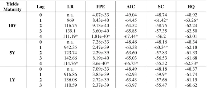
Thus, the first step was to determine the optimal lag length considering the frequency of the data sample as well as the information criteria, for each of our three models mentioned above. As about the first approach, we considered four lags as relatively reasonable since our data sample is in quarterly frequency (Pesaran and Pesaran, 2009). Regarding information criteria, the optimal lag is not unanimous as some indicate four as the optimal lag while others indicate three (Table 4). However, we choose four lags, as this was the choice of the majority of information criteria but also for considering that FPE and AIC criteria are better indicators in the case of relatively small samples sizes (Khim and Liew, 2004). In addition, we also considered an unrestricted VAR with five lags and ran the stability condition check for the ten-year maturity government bond yields and the results proved that it did not satisfy the stability condition with a higher number of lags – at least one characteristic polynomial root is outside the unit circle (Lütkepohl, 2005).2
Table 4 - Values of information criteria Yields
Maturity Lag LR FPE AIC SC HQ
0 n.a. 4.07e-33 -49.04 -48.74 -48.92 1 969 8.43e-40 -64.45 -61.42* -63.26* 10Y 2 116.75 9.13e-40 -64.52 -58.75 -62.24 3 139.1 3.60e-40 -65.85 -57.35 -62.50 4 111.19* 1.81e-40* -67.44* -56.2 -63.01 0 n.a. 7.28e-33 -48.46 -48.16 -48.34 1 942.35 2.47e-39 -63.38 -60.34* -62.18 5Y 2 123.74 2.29e-39 -63.60 -57.83 -61.33 3 142.66 8.19e-40 -65.03 -56.53 -61.68 4 114.76* 3.6e-40* -66.75* -55.52 -62.33* 0 n.a. 7.09e-33 -48.49 -48.18 -48.37 1 916.86 3.85e-39 -62.93 -59.9* -61.74 1Y 2 136.08 2.72e-39 -63.43 -57.66 -61.15 3 110.59 2.37e-39 -63.97 -55.47 -60.62
22
4 131.53* 5.6e-40* -66.31* -55.07 -61.88*
Note: * indicates the optimal lag order selected by the respective criteria
Hence, we ran an ARDL on EViews software (9.5 version) considering four maximum lags and no trend specification, being the optimal number of lags (up to a maximum of four) defined automatically for each variable by the software. The reason why we did not consider trend was because our dependent variables did not show any evidence of it (figures 2, 3 and 4 in the Appendix).
After running the models, we then assessed the existence of a cointegration relationship between our variables by conducting the F-Bounds test (Table 5). The computed F-statistics considering all the three sovereign bonds yields maturities proved to be higher than the upper bound critical values at the traditional significance levels, which means there is evidence supporting the existence of a cointegration relationship between the variables (i.e., rejection of the null hypothesis of no cointegration).
Table 5 - Bounds test for cointegration analysis (short version)
Yields
Maturity F-statistic Critical Value
Lower Bound Value Upper Bound Value 8.551 10Y 1% 2.62 3.77 10.789 5Y 5% 2.11 3.15 3.491 10% 1.85 2.85 1Y
Note: The lower and upper bound values regarding each significance level are the same for the different bonds yields maturities.
We then performed four diagnostic tests in order to assess the adequacy, reliability and completeness of each of our three models, as shown in table below (Table 6).
Table 6 - Diagnostic tests for ARDL estimations Yields
Maturity Test F-statistic P-value
10Y Autocorrelation 0.142 0.709 Ramsey’s RESET 1.635 0.2 Normality n. a. 0.822 Heteroscedasticity 1.354 0.249 5Y Autocorrelation 0.001 0.977 Ramsey’s RESET 3.319 0.03 Normality n.a. 0.673 Heteroscedasticity 0.582 0.449 1Y Autocorrelation 0.4 0.532
23
Ramsey’s RESET 13.169 0.0003
Normality n.a. 0.431
Heteroscedasticity 2.768 0.101 Note: F-statistic represents the LM F or ‘modified LM’ statistic.
The results are conclusive and show the adequacy of our models. First, they do not show evidence of autocorrelation as we cannot reject the null hypothesis of lack of autocorrelation in the residuals. There is also evidence that the ten and five years maturities models are well specified in their functional form as we also cannot reject the null hypothesis of Ramsey’s test. Finally, the results indicate that residuals are normally distributed and homoscedastic. It is also worth noting that the conclusions were the same considering a higher number of lags, regarding the autocorrelation and the heteroscedasticity tests.
We then performed CUSUM and CUSUMSQ tests, whose figures (Figures 13 to 18 in the Appendix) indicate that the coefficients are stable over the sample period and thus confirming the absence of structural breaks, as the recursive residuals lie within the straight lines4 (at 5%
significance levels).
Moreover, it is also worth noting that estimation outputs present R-squared valuesof 0.992, 0.99 and 0.968 (ten, five and one year maturities, respectively) meaning that all the models fit well the data sample. In short, we conclude that the estimated ARDL models do not present any econometric problem.
By analyzing the ten-year maturity sovereign bond yields long-term equation (Table 7), we conclude that all variables are statistically significant at the traditional significance levels and that most of the coefficients have the expected signs and are in line with the related literature. The only exception is the public debt (PD) variable, which shows not to have the expected sign, by turning out to be negative determinant of the yields. Nevertheless, it is worth noting that the effects of government debt on long-term interest rates are dependent on its funding sources: either in domestic or in foreign investors - in Portugal’s case, a large part of the public debt is placed on foreign entities instead of domestic investors. According to this argument, when a country depends less on foreign borrowing, long-term interest rates are lower, since investors
3 Although the test for the one-year maturity suggests that the model is not in its correct functional form,
it should be noted that the Ramsey’s test should only be applied when estimators are carried out by the OLS estimators, which is not our case (Agung and Ngurah, 2009).
4Regarding one-year government bond yields maturity, despite the CUSUMSQ test revealing that the
recursive residuals lie outside the critical bounds for the period from 2010q2 to 2011q2, the CUSUM test confirms the stability of the model as the recursive residuals lie within the straight lines for all the data sample.
24
more firmly form the perception that government has a strong incentive to avoid defaulting (Ichiue, 2012). Thus, from this point of view, external debt tend to be a more relevant factor than public debt, which can be a possible explanation to the contradictory sign of the latter one.
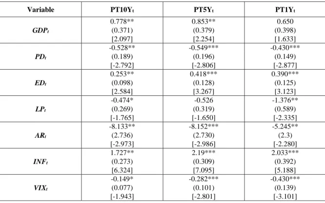
In short, GDP, ED, INF and L are positive determinants of the ten-year maturity government bond yields. For instance, a 1 p.p. rise in GDP increases the yields by around 77,8 basis points. On the other hand, the variables PD, LP, AR and VIX influence government bonds yields in a negative way. For example, a 1 p.p. increase in the public debt lowers the yields by 52,8 basis points.
Regarding the five-year maturity sovereign bond yields (Table 7), we conclude that the signs remain the expected ones and that the magnitude of impacts turn out to be not so different when compared to the ten year maturity bond yields. However, labour productivity (LP) ceases to be statistically relevant even at 10% significance level, which means it is not considered as an explanatory variable for the five-year maturity government bond yields – thus, we conclude that investors do not consider this variable to assess the country default risk in the medium term.
As about the estimation for the one year maturity sovereign bond yields (Table 7), GDP growth rate (GDP) and liquidity (L) revealed not to be statistically relevant but the remaining six variables kept being statistically relevant and with the signs in line with the higher bond yields maturities.
Table 7 - Long-term estimations of sovereign bond yields
Variable PT10Yt PT5Yt PT1Yt
GDPt 0.778** 0.853** 0.650 (0.371) (0.379) (0.398) [2.097] [2.254] [1.633] PDt -0.528** -0.549*** -0.430*** (0.189) (0.196) (0.149) [-2.792] [-2.806] [-2.877] EDt 0.253** 0.418*** 0.390*** (0.098) (0.128) (0.125) [2.584] [3.267] [3.123] LPt -0.474* -0.526 -1.376** (0.269) (0.319) (0.589) [-1.765] [-1.650] [-2.335] ARt -8.133** -8.152*** -5.245** (2.736) (2.730) (2.3) [-2.973] [-2.986] [-2.280] INFt 1.727** 2.19*** 2.033*** (0.273) (0.309) (0.392) [6.324] [7.095] [5.188] VIXt -0.149* -0.282*** -0.430*** (0.077) (0.101) (0.139) [-1.943] [-2.801] [-3.101]
25 Lt 35.709** 27.136** 12.335 (14.505) (12.825) (14.046) [2.462] [2.116] [0.878] 5.575** 5.669*** 3.796** β0 (1.867) (1.884) (1.568) [2.986] [3.008] [2.420]
Note: Standard errors in (), z-statistics in [], *** indicates statistical significance at 1% level, ** indicates statistical significance at 5% level and * indicates statistical significance at 10% level.
Moreover, we re-estimated the long version of the ten-year maturity model replacing external net debt (ED) for external gross debt (EGD), in order to check the robustness of the model. The objective is to ensure the main results are not affected by considering different variables. Yet, reported estimation results5 allowed us to conclude that the main conclusions remain unchanged as the variables kept being cointegrated and external gross debt (EGD) continued to influence negatively the government bond yields.
By analyzing the ten-year maturity sovereign bond yields short-term equation (Table 8), we conclude that the coefficient of the error correction term is negative and significant at 1% significance level, which reinforces the stability and adequacy of the model and its convergence to the long-term equilibrium. All variables are statistically significant for the majority of lags, with only a few presenting contradictory signs when compared to long-term estimations. That is the case of public debt (PD) and external debt (ED) that appears to influence the yields positively and negatively, respectively. Regarding the first one, and unlike long-term estimations, we find here evidence supporting the claim that public debt influences positively sovereign bond yields – therefore having the expected sign in the short-term.
As about the other bonds yields maturities (Tables 9 and 10), results also confirm the convergence of both short-term models to their long-term equilibrium at 1% significance level.
However, liquidity (L) seems to be no longer a relevant factor in evaluating both short and medium term sovereign bonds yields. A possible explanation may be that is less riskier a country to default as the maturity decreases, as investors will hold the securities for lesser time - therefore they prefer to look at other factors besides liquidity in the short-term.
Moreover, external debt (ED) ceases to be statistically relevant to determine one-year maturity bond yields but kept explaining the medium term yields. By looking at the results, it seems that investors prefer to look at public debt instead of external debt in the short-term, as the first one kept being relevant on the majority of lags even at 1% significance level.
26
Table 8 - Short-term estimations of the ten-year maturity government bond yields Variable Coefficient Standard Error T-statistic
∆PT10Yt-1 0.359*** 0.072 4.983 ∆GDPt 0.207*** 0.056 3.675 ∆GDPt-1 -0.075 0.059 -1.286 ∆GDPt-2 -0.297*** 0.057 -5.243 ∆PDt 0.030 0.042 0.723 ∆PDt-1 0.235*** 0.045 5.225 ∆PDt-2 0.127*** 0.021 5.901 ∆PDt-3 0.097*** 0.023 4.187 ∆EDt -0.044** 0.020 -2.162 ∆EDt-1 -0.073*** 0.022 -3.334 ∆EDt-2 -0.036 0.024 -1.536 ∆EDt-3 -0.073*** 0.022 -3.294 ∆LPt -0.125** 0.058 -2.179 ∆LPt-1 -0.070 0.054 -1.286 ∆LPt-2 0.20*** 0.052 3.822 ∆ARt -0.742*** 0.245 -3.032 ∆ARt-1 1.054*** 0.245 4.306 ∆ARt-2 0.397 .0245 1.619 ∆ARt-3 -0.444** 0.198 -2.24 ∆INFt 0.183** 0.081 2.253 ∆INFt-1 -0.061 0.092 -0.663 ∆INFt-2 -0.483*** 0.083 -5.796 ∆VIXt -0.020** 0.008 -2.527 ∆VIXt-1 0.042*** 0.008 5.256 ∆VIXt-2 0.011 0.007 1.455 ∆Lt 2.866 2.215 1.294 ∆Lt-1 -7.539*** 2.288 -3.295 CoIntEqt-1 -0.316*** 0.029 -10.678
Note: ∆ is the operator of the first differences, *** indicates statistical significance at 1% level, ** indicates statistical significance at 5% level and * indicates statistical significance at 10% level
Table 9 -Short-term estimations of the five-year maturity government bond yields Variable Coefficient Standard Error T-statistic
∆PT5Yt-1 0.542*** 0.061 8.862 ∆GDPt 0.105 0.077 1.358 ∆GDPt-1 -0.108 0.084 -1.284 ∆GDPt-2 -0.403*** 0.080 -5.022 ∆PDt -0.042 0.029 -1.439 ∆PDt-1 0.154*** 0.030 5.098 ∆PDt-2 0.258*** 0.031 8.278 ∆PDt-3 0.169*** 0.034 4.989 ∆EDt 0.031 0.030 1.036 ∆EDt-1 -0.042 0.028 -1.478 ∆EDt-2 -0.114*** 0.030 -3.753 ∆EDt-3 -0.097*** 0.031 -3.131 ∆LPt -0.154* 0.083 -1.848 ∆LPt-1 -0.105 0.080 -1.310 ∆LPt-2 0.229*** 0.075 3.038 ∆ARt -1.343*** 0.302 -4.441 ∆ARt-1 0.479* 0.278 1.721 ∆ARt-2 0.043 0.284 0.154 ∆ARt-3 -0.645** 0.264 -2.245 ∆INFt 0.032 0.114 0.280 ∆INFt-1 0.045 0.130 0.349
27 ∆INFt-2 -0.836*** 0.117 -7.144 ∆VIXt -0.055*** 0.012 -4.690 ∆VIXt-1 0.068*** 0.012 5.768 ∆VIXt-2 0.021* 0.011 1.980 CoIntEqt-1 -0.369*** 0.031 -11.890
Note: ∆ is the operator of the first differences, *** indicates statistical significance at 1% level, ** indicates statistical significance at 5% level and * indicates statistical significance at 10% level
Table 10 - Short-term estimations of the one-year maturity government bond yields
Variable Coefficient Standard Error T-statistic
∆PT1Yt-1 0.577*** 0.095 6.087 ∆PT1Yt-2 0.472*** 0.115 4.122 ∆PT1Yt-3 -0.211** 0.097 -2.163 ∆GDPt 0.224* 0.132 1.699 ∆GDPt-1 -0.265* 0.130 -2.035 ∆GDPt-2 -0.384*** 0.127 -3.023 ∆PDt -0.068 0.050 -1.365 ∆PDt-1 0.382*** 0.045 8.454 ∆PDt-2 0.260*** 0.057 4.561 ∆PDt-3 -0.180*** 0.058 -3.112 ∆EDt 0.042 0.047 0.891 ∆LPt -0.537*** 0.149 -3.613 ∆LPt-1 -0.032 0.121 -0.263 ∆LPt-2 0.396*** 0.126 3.153 ∆LPt-3 0.399*** 0.110 3.630 ∆ARt -1.346*** 0.475 -2.837 ∆INFt 0.347* 0.181 1.915 ∆INFt-1 -0.645*** 0.217 -2.971 ∆INFt-2 -0.591*** 0.207 -2.858 ∆VIXt -0.095*** 0.021 -4.443 ∆VIXt-1 0.051** 0.020 2.630 CoIntEqt-1 -0.444*** 0.067 -6.666
Note: ∆ is the operator of the first differences, *** indicates statistical significance at 1% level, ** indicates statistical significance at 5% level and * indicates statistical significance at 10% level
Finally, we present the economic significance of our statistically significant estimates in order to correctly identify the drivers of the Portuguese government bond yields over the period from 2000 to 2016. In addition, we also present the economic effects regarding two distinct periods: i) Pre-Crisis (2000q1 to 2009q4) and ii) Crisis and Post-Crisis (2010q1 to 2016q4). The results are presented in table below (Table 11).
Table 11 - Economic significance of our estimates for Portuguese government bond yields by maturity
Period Yields Maturity Variable Long-term Coefficient Actual Cumulative Change Economic Effect
Full Period 10Y
GDPt 0.778 -0.538 -0.419 PDt -0.528 1.513 -0.799 EDt 0.253 3.807 0.963 LPt -0.474 -0.838 0.397 ARt -8.133 0.039 -0.32 INFt 1.727 -0.572 -0.988 VIXt -0.149 -0.391 0.058
28 Lt 35.709 0.901 32.16 5Y GDPt 0.853 -0.538 -0.459 PDt -0.549 1.513 -0.831 EDt 0.418 3.807 1.591 ARt -8.152 0.039 -0.318 INFt 2.19 -0.572 -1.253 VIXt -0.282 -0.391 0.11 Lt 27.136 0.901 24.45 1Y PDt -0.430 1.513 -0.651 EDt 0.390 3.807 1.485 LPt -1.376 -0.838 1.153 ARt -5.245 0.039 -0.205 INFt 2.033 -0.572 -1.163 VIXt -0.430 -0.391 0.168 Pre-Crisis 10Y GDPt 0.778 -1.289 -1.003 PDt -0.528 0.611 -0.323 EDt 0.253 3.218 0.814 LPt -0.474 -0.473 0.224 ARt -8.133 0.031 -0.252 INFt 1.727 -1.384 -2.39 VIXt -0.149 -0.003 0.00 Lt 35.709 0.523 18.676 5Y GDPt 0.853 -1.289 -1.100 PDt -0.549 0.611 -0.335 EDt 0.418 3.218 1.345 ARt -8.152 0.031 -0.253 INFt 2.19 -1.384 -3.031 VIXt -0.282 -0.003 0.001 Lt 27.136 0.523 14.192 1Y PDt -0.430 0.611 -0.263 EDt 0.390 3.218 1.255 LPt -1.376 -0.473 0.651 ARt -5.245 0.031 -0.163 INFt 2.033 -1.384 -2.814 VIXt -0.430 -0.003 0.001 During and Post-Crisis 10Y GDPt 0.778 -0.008 -0.006 PDt -0.528 0.513 -0.271 EDt 0.253 0.129 0.033 LPt -0.474 -0.823 0.39 ARt -8.133 0.001 -0.008 INFt 1.727 1.629 2.813 VIXt -0.149 -0.301 0.045 Lt 35.709 0.229 8.177 5Y GDPt 0.853 -0.008 -0.007 PDt -0.549 0.513 -0.282 EDt 0.418 0.129 0.054 ARt -8.152 0.001 -0.008 INFt 2.19 1.629 3.568 VIXt -0.282 -0.301 0.085 Lt 27.136 0.229 6.214 1Y PDt -0.430 0.513 -0.221 EDt 0.390 0.129 0.05 LPt -1.376 -0.823 1.132 ARt -5.245 0.001 -0.005 INFt 2.033 1.629 3.312 VIXt -0.430 -0.301 0.129
Note: The actual cumulative change corresponds to the growth rate of the correspondent variable. The economic effect is the multiplication of the long-term coefficient by the actual cumulative change.
29
Regarding the full period, external debt, labour productivity and liquidity were the variables that had a prejudicial impact on the ten-year maturity sovereign bond yields.
Within these, external debt had one of the worst impacts since its increase favored an acceleration of the yields by around 96,3 per cent. On the other hand, activity rate, GDP, public debt and inflation rate had a beneficial impact on Portuguese sovereign bond yields with ten years maturity. The variable that most benefited the yields was the inflation rate, as its negative variation contributed to a decrease on government funding costs by 98,8 per cent. As about the government bond yields with five year maturity, it is important to mention that external debt and inflation caused an even greater impact on the yields – the increase of external debt made the yields grew up by 159,1 per cent whilst the decrease of inflation contributed to lower the government bond yields by 125,3 per cent. In line with the ten-year maturity government bonds, the external debt and inflation rate had a similar effect but presented a greater impact on one-year maturity sovereign bond yields. Additionally, the most important effect that deserves to be highlighted is the decrease on labour productivity which caused the yields to rise by 115,3 per cent.
Thus, between 2000 and 2016, a fact that it is worth being highlighted is that the beneficial impact caused by public debt was not enough to compensate the upward pressure on the yields induced by external debt.
Considering the Pre-Crisis period, external debt, labour productivity and liquidity were again the more important determinants that contributed to the raise of the ten-year maturity sovereign borrowing costs. On the other hand, public debt, activity rate, GDP and inflation rate were the risk drivers that contributed to the decrease of the Portugal cost of debt, with the latter two causing the major impact. Moreover, despite the positive variation of external debt that contributed to the increase of ten year maturity sovereign bond yields by 81,4 per cent, the negative variation of inflation rate was enough to compensate it, as it contributed to the reduction of the yields by 239,0 per cent. Furthermore, the stock market volatility proved to have a residual effect in the Pre-Crisis period since its variation considering the different maturities was close to zero – thus confirming the theoretical idea that in non-crisis periods the market volatility tend to be smaller when compared to periods of financial turnoil.
In this way, during the Pre-Crisis period, the impact on yields seemed to be more through economic fundamentals such as GDP and inflation rate instead of fiscal conditions, as the positive variation of public debt only contributed to lower the yields by 32,4 per cent in that
30
period (thus, corroborating the idea that there are less concerns about the country’s debt during non crisis periods).
Regarding the five-year government bond yields maturity, the impacts are similar except for the external debt and inflation rate whose impact revealed to be greater when compared with the longer-term government bonds maturity. Accordingly, the increase of external debt made the government bonds yields grew up by 134,5 per cent while the decrease on inflation rate made the yields fall by 303,1 per cent on the period. As about the one-year maturity, only labour productivity is worth highlighting for its greater impact since the other effects are quiet similar when compared with the higher bonds yields maturities. Thus, the negative variation of labour productivity made the yields grew up by 65,1 per cent.
During and after the crisis, there is evidence that public debt was the main driver on ten year maturity sovereign bond yields, since the anemically negative variations of GDP and activity rate evidenced an effect close to zero on the yields. In turn, liquidity, labour productivity but mostly inflation rate had the worst impact on the yields. Regarding the latter one, its positive variation in the period contributed to a 281,3 per cent increase on the ten year maturity bond yields. Considering the five year maturity yields, liquidity and inflation rate were the determinants that had the most harmful impact, with the positive variation of the latter one leading to a 356,8 per cent increase on the yields.
As about the yields with the lowest maturity, the variable with the greatest impact was once again the inflation rate with the other variables keep exerting an identical effect except the labour productivity. In fact, labour productivity played a more important role comparing to the ten-year maturity government bonds yields since its decrease during and after the crisis led the yields to grow by 113,2 per cent.
To sum up, the Portuguese government bonds yields were essentially harmful affected by liquidity, labour productivity but mostly by external debt. In turn, activity rate, GDP and public debt proved to have a beneficial effect on those yields with the decrease of inflation rate having the greatest positive impact. However, in crisis and post crisis period, the inflation rate has shown to present a contradictory effect since its increase within this period exerted a prejudicial effect on the Portuguese sovereign bonds yields.
32
VII. Conclusion
This paper presented an empirical analysis on the main determinants of the Portuguese government bonds yields, considering different maturities, for the period between 2000 and 2016 using quarterly data.
The usual factors used to estimate government bond yields are macroeconomic performance, fiscal conditions, inflation rate as well as global aversion and liquidity risks. A few studies indicate foreign borrowing, labour productivity and demographics as factors that may also influence sovereign funding costs.
An equation for sovereign bond yields using quarterly data between 2000 and 2016 was estimated using eight independent variables such as GDP growth rate, public debt, external debt, labour productivity, activity rate, inflation rate, stock market volatility and liquidity. We not only estimated the ten-year maturity government bonds as we also estimated for the five and one year maturities in order to check how the explanatory variables affect the medium and the short-term sovereign borrowing costs.
Since the variables were integrated of order zero and of order one, the ARDL methodology was followed. The model presented the distinction between the long run effect and the short run effect of those variables on the government bond yields.
Our main findings relative to the long run were that GDP growth rate, external debt, inflation rate and liquidity influence the yields positively while public debt, labour productivity, activity rate and the stock market volatility are negative determinants of sovereign bond yields. The greatest finding was that the public debt presents a contradictory sign to what the majority of literature claims since an increase on public debt lowers the government bond yields. Additionally, as the yields maturities decrease we conclude that some variables stopped being statistically relevant.
Overall, the main results point out that there were no significant differences regarding the long-term delong-terminants of the government bonds yields among the different maturities considered.
In the short run, most of the statistically significant lagged variables presented identical signs when compared to long run estimations. Moreover, liquidity showed not to be a relevant factor to evaluate both medium and short term sovereign bonds yields while external debt also ceased to be statistically relevant to explain the latter one.