Bayesian networks in forensic identification problems

(1)

BAYESIAN NETWORKS

IN FORENSIC IDENTIFICATION PROBLEMS

ANDRADE Marina, (P), FERREIRA Manuel Alberto M., (P)

Abstract. Paternity dispute and criminal identification problems are examples of situations in

which forensic approach the DNA profiles study is a common procedure. In order to deal with the problems mentioned it is needed an introduction to present and explain the various concepts involved, since distinct areas must be considered. In the second paragraph some problems are presented. Here it is exhibited an algebraic treatment, for the simpler problems and with those the use of the object-oriented Bayesian networks is shown. Then the most complex kind of problems that may occur is presented. In the last paragraph some comments are added.

Key words: Bayesian networks, DNA profiles, identification problems. Mathematics Subject Classification: Primary 62C10; Secondary 62P99.

1 Introduction

The use of networks transporting probabilities began with the geneticist Sewall Wright in the beginning of the 20th century (1921). Since then their use had different forms in several areas like social sciences and economy – in which the used models are, in general, linear named Path Diagrams or Structural Equations Models (SEM), and in artificial intelligence – usually non-linear models named Bayesian networks also called Probabilistic Expert Systems (PES).

Bayesian networks are graphical structures for representing the probabilistic relationships among a large number of variables and for doing probabilistic inference with those variables, Neapolitan (2004). Before we approach the use of Bayesian networks to our interest problems we briefly discuss some aspects of PES in connection with uncertainty problems.

1.1 Probability concept

The interpretation of probability has been and still is a subject of intense debate. It has important implications for the practice of probability modelling and statistical inference, both in general and

(2)

Aplimat – Journal of Applied Mathematics

volume 2 (2009), number 3

14

in expert systems applications. We believe that the main division may be stated between objective and epistemological, Gillies (1994), understandings of P(A), the probability of the event A; or more generally of P(A|B), the probability of A conditional on the happening of the event B.

Objective theories consider such probabilities as real world attributes of the events they refer to, and are not affected by or related to our perception of them. The most influent objective interpretation has been the frequentist interpretation (Venn; von Mises, Reichenbach, etc.), to which probability is defined as the limit of the proportion of successes in an infinite sequence of experiments. It only allows the approach of repeatable events. Despite this important limitation this interpretation has been the dominant one and was the basis of Neyman and Pearson’s frequentist approach to statistical inference.

Epistemological theories see P(A|B) as a state of mental uncertainty about A, in the knowledge of B – where A and B may be singular propositions and not necessarily repeatable events. These theories can be divided into logical and subjectivists theories. Logical theories suppose the existence of a single rational degree of uncertainty about A, in the knowledge of B. However, the problem is that it is not yet known a method for the evaluation of logical probabilities. The subjectivist interpretation has become more popular in the last years. Subjectivists regard probability as a degree of reasonable belief in a certain event, from an individual viewpoint; therefore probability is a numeric subjective measure of a particular person according his/her degree of belief, as long as it is ‘coherent’1.

Obviously, from the objective part the critics can claim that it is an extremely vulnerable assertion. However, experience shows that distinct people, with different degrees of knowledge or information with respect to certain events, have different quantifications of the associated uncertainty.

From a subjectivist perspective it is possible to specify probabilities of individual propositions, and even to treat unknown constants or parameters as random variables. Being unknown it is possible to assign them probabilities, under a coherent structure. The subjectivist interpretation is the one we follow here.

1.2 Expert systems

Expert systems are attempts to crystallize and codify the knowledge and skills of one or more experts into a tool that can be used by non-specialists, Cowell et al. (1999). An expert system can be decomposed as follows:

Expert system = knowledge base + Inference engine.

The first term on the right-hand side of the equation, knowledge base, refers the specific knowledge domain of the problem. The inference engine is given by a set of algorithms, which process the codification of the knowledge base jointly with any specific information known for the application in study.

1_{The principle of coherence requires that an individual should not make a collection of probability assessments that}

could put him in the position of suffering a sure loss, no matter how the relevant uncertain events turn out, Cowell et al. (1999).

(3)

volume 2 (2009), number 3 15

Usually it is presented in a software program, as the one we are going to show hereafter, but such is not an imperative rule. Each of those parts is important for the inferences, but knowledge base is crucial. The inferences obtained depend naturally on the quality of the knowledge base, of course in association with a sophisticated inference engine. The better those parts are the best results we can get.

A PES is a representation of a complex probability structure by means of a directed acyclic graph, having a node for each variable, and directed links describing probabilistic causal relationships between variables, Dawid et al. (2002). Bayesian approach is the adequate for making inferences in probabilistic expert systems.

1.2.1 Bayesian networks

Bayesian networks are graphical representations expressing qualitative relationships of dependence and independence between variables. A Bayesian network is a directed acyclic graph G (DAG) having a set of V vertices or nodes and directed arrows. Each node υ є V represents a random variable Xυ with a set of possible values or states. The arrows connecting the nodes describe conditional probability dependencies between the variables.

The set of parents, pa(υ), of a node υ comprises all the nodes in the graph with arrows ending in υ. The probability structure is completed by specifying the conditional probability distributions for each random variable Xυ and each possible configuration of variables associated with its parent nodes xpa(υ). The conditional distribution of Xυ is expressed given Xpa(υ) = xpa(υ). The joint distribution is p(x) = Π υєV p(x υ| xpa(υ)). There are algorithms to transform the network into a new graphical representation, named junction tree of cliques, so that the conditional probability p(x υ| xA) can be efficiently computed, for all υ є V, any set of nodes A⊆ , and any configuration xV A of the nodes XA. The nodes in the conditioning set A are generally nodes of observation and input of evidence XA= xA, or they may specify hypotheses being assumed.

Software such as Hugin2 can be used to build the Bayesian network through the graph G. That can be done by specifying the graph nodes, their space of states and the conditional probabilities p(x υ| xpa(υ )). In the compiling process the software will construct its internal junction tree representation. Then, by entering the evidence XA= xA at the nodes in A, and requesting its propagation to the remaining nodes in the network, the conditional probabilities p(x υ| xA) are obtained.

OOBN are one example of the general class of Bayesian networks. An instance or object is a regular network possessing input and output nodes as well as ordinary internal nodes. The interface nodes have grey fringes, with the input nodes exhibiting a dotted line and the output nodes a solid line. The instances of a given class have identical conditional probability tables for non-input nodes. The objects are connected by directed links from output to input nodes. The links represent identification of nodes. We use bold face to refer the object classes and math mode to refer the nodes. The modular flexibility structure of the OOBN is of great advantage in complex cases

(4)

16

1.2.2 STR markers and DNA profiles

The development of the molecular biology, since the decade of 60, allowed the knowledge of the DNA structure and its implementation as a genetic information vehicular, so that it can also be used in the clarification of judicial forensic problems.

Every human being has 23 pairs of chromosomes in the nuclear of human cell. One of those pairs determines the gender – XY for male, XX for female. The other 22 pairs are said homologous pairs. All of them are DNA molecules. A DNA molecule is a double helix composed by four different nucleotides: C, A, G and T, binding in pairs C-G and A-T.

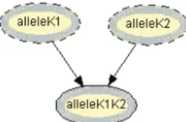
A locus, sometimes also named a gene for simplification, is an area on a chromosome and the DNA composition on that area is an allele. Thus, a locus corresponds to a random variable and the allele is its realized state.

A DNA marker is a known locus where the allele can be measured in the laboratory, by the use of appropriate techniques. More recently, the techniques provide the use of Short Tandem Repeats (STR) markers, which avoid the possibility of measurement errors. STR markers are given by integers, but they can be codified even to protect the process or case. If an STR allele exhibits a value of 5, a certain expression (e.g. GTCCAG) is repeated exactly five times at that locus.

A DNA profile for an individual is a measurement on several markers to which a genotype is observed. The genotype is an unordered pair of alleles, one inherited from the individual’s father and the other from the mother, although it is not possible to distinguish which is which. In this work we implement the product rule that is Hardy-Weinberg and linkage equilibrium assumptions; in practice it assumes the independence of the individual’s alleles both within and across markers. If a more complex genetic model was desired it could be implemented by introducing dependencies between founder nodes.

1.3 Forensic identification

The use of DNA profiles in forensic identification problems has become, in the last years, an almost regular procedure in many and different situations. Among those are: 1) disputed paternity problems, in which it is necessary to determine if the putative father of a child is or is not the true father; 2) criminal cases as if a certain individual A was the origin of a stain found in the scene of a crime; or 3) in more complex cases to determine if an individual or more did contribute to a mixture trace found. In criminal cases it is common to find traces with more than one single contributor. As it is known a person has at most two different alleles for each marker. If a trace exhibits more than two alleles to one or more markers then it is certainly a mixture trace.

Mixture traces can happen in rape cases, where the vaginal swab typically will contain DNA from the victim as well as the perpetrator, and also from a consensual partner or several perpetrators. Homicides or robberies are other possible origin for mixture traces, where we can admit a fight that produces some material.

(5)

There are still some other forensic identification problems, however not too frequent ones. That is the case of an identification of a body found, together with is information of a missing person belonging to a known family, or the identification of more than one body resultant of a disaster or an attempt. And even immigration cases in which it is important to establish family relations. We can say that the use of Bayesian arguments in forensic problems begun with a Dennis Lindley work in 1977. Since then there is a huge amount of published works in this area, in great part due to the evolution of the DNA profiling techniques. The interest in forensic identification problems was not exclusively of forensic scientists as it can be seen by innumerable articles made with the contribution of statisticians.

2 Using Bayesian networks

Dawid et al.'s (2002) work describes a new approach to the problems mentioned above. The construction and use of Bayesian networks to analyse complex problems of forensic identification inference was initially done there followed by Evett et al. (2002), Dawid et al. (2002), Mortera (2003) and Mortera et al. (2003) among others.

Here we start with a simple graphical and numerical representation and extend our analysis to more complex problems, such as DNA mixtures and cases where the evidence is composed with more than one trace.

2.1 Disputed paternity

In a case of disputed paternity the genetic information of the child can be seen as partial information about the true father. In a simple case the paternity is imputed to a certain individual who rejects it. DNA profiles of the mother m, the child c, and the putative father pf are available.

Becoming the paternity assumption litigious we can say that, in formal terms, two hypotheses are established, which for simplification we will name the prosecution and the defense hypotheses, i.e., HP: The true father is the putative father.

vs

HD: The true father is another individual randomly drawn from the population, and not genetically related with the mother or the putative father.

We need to assess the likelihood function over the hypotheses as to the true father. If we denote the data (mgt, cgt, pfgt) as the evidence E, then we want to evaluate the likelihood ratio:

(

)

(

D

)

P H E P H E P LR | | = .

(6)

18

Naturally the court has to answer to the truly paternity of the child. If we want the court has to evaluate the ratio of the hypotheses in dispute. That is

(

)

(

)

(

|

)

( )

. | | | D P D P D P H P H P H E P H E P E H P E H P × =

If we admit thatP

( )

H_P =P

( )

H_D then

(

)

(

)

(

D

)

P D P H E P H E P E H P E H P | | | | = .

Before continuing let us briefly explain the equations above.

Being the markers in different chromosomes (linkage equilibrium) and assuming random mating (Hardy-Weinberg equilibrium) we have independence between and within markers. Therefore we can obtain the LR for each marker separately and multiply the values to determine the overall likelihood ratio based on the data available for all markers.

We want to determine the probability of the triplet E, under the two hypotheses. We can agree that before knowing any data on the child it is reasonable to assume that the identity of the true father is independent of the mother’s and the putative father’s. And supported on that, it is easily seen that we can determine the conditional probability of the child’s genotype, given the other two available genotypes. Thus, to determine P

(

E|H_P

)

we simply have to apply the Mendel’s laws. But the calculus of P

(

E|H_D

)

necessarily demands the knowledge of the population allele frequencies for the considered markers.

Let us admit that for a certain marker the triplet E = (mgt, gtc, pfgt) is the following

(

) (

)

(

A B B B A B

)

E = , ; , ; , , and pA and pB are the population allele frequencies for the considered marker.

(

)

[

(

) (

)

]

(

)

[

]

5 . 0 5 . 0 ; | ; | ; ; | × = = = pfgt mgt cgt P pfgt mgt pfgt cgt mgt P H E P _P and

(

)

[

(

) (

)

]

(

)

[

]

B P p rgt mgt cgt P rgt mgt pfgt cgt mgt P H E P × = = = 5 . 0 ; | ; | ; ; |

where rgt assigns the genotype of a random individual of the population, not related to the mother or the putative father.

(7)

Aplimat – Journal of Applied Mathematics volume 2 (2009), number 3 19

(

)

(

)

. 5 . 0 | | B D P p H E P H E P LR = =

The considered problem is, as shown, easily algebraically solved. However we will use it to illustrate the simplicity and the advantages of using this tool in more complex situations. Given the freedom of choice for the variables to include in the graphical representation, different representations can be obtained. Some of them simpler than others. To get a ‘good’ representation is very important to the efficiency and the viability of the computational routines. These are extremely sensible to the organization of the graphical structure. The first step consists on the identification and definition of the nodes for all the variables of interest to the problem.

After that we are able to build the graph representation. In accordance with Dawid et al. (2002), in order to maximize the efficiency of the calculations as well as the logical clarity of the representation we chose to disaggregate each individual’s genotype into its constituent, unobserved, paternally and maternally inherited genes.

Thus, in Fig. 1 we have the OOBN for the paternity case discussed in Dawid et al. (2002), considering a single marker. Each node (instance) in the network represents itself a Bayesian network. In this simple paternity case instances pfmg, pfpg, mpg and mmg are all of class founder, Fig. 2, and represent the ‘putative father’s maternal and paternal gene’, and similarly for the mother. Instances mgt, cgt and pfgt are of class genotype, Fig. 3, and consider the observed genotype. The instances tfmg and tfpg are of class whom, Fig. 4, and specify whether the correspondent allele is or is not from the putative father. And cpg and cmg of class inherit, Fig. 5 represent the allele transmission through meiosis. The node tf=pf? represents the binary query ‘Is the true father the putative father?’

Figure 1: Simple paternity network.

The instance founder contains a single node gene, having for its space of states all the possible alleles that can be presented for the specific case, and the correspondent population gene frequencies.

(8)

20

Figure 2: founder network.

The genotype of an individual is an unordered pair of alleles inherited from paternal, pg, and maternal, mg, genes, here represented by gtmin:=min{pg, mg} and gtmax:=max{pg, mg}, where pg and mg are input nodes identical to the gene node of founder.

Figure 3: genotype network.

The instance whom describes the true father’s allele origin. If tf=pf? has true for value then the true father’s allele, tfg, will be identical with the putative father’s, pfg, otherwise the true father’s allele is chosen randomly from another man in the population, with otherg an instance of the class founder, and tfg:=if(tf=pf?= = true, pfg, otherg.gene).

Figure 4: whom network.

The network models the Mendel’s inheritance in which the child’s allele is chosen at random from the two parents, pg and mg, here as the sequence of the observed outcome of a fair coin toss. The node coin is modeled as a Binomial(1, 0.5), therefore cg:= if(fcoin.coin = =1, pg, mg).

(9)

Following Dawid et al. (2002), the data for marker FES are child genotype cgt = {12, 12}, mother’s genotype mgt = {10, 12} and putative father’s genotype = {10, 12}. The population allele frequencies are p10 = 0.28425 and p12 = 0.25942. As the authors point out, this simple problem can be easily handled by an algebraic approach. But, the interest in it is to illustrate the simplicity and advantages of using this tool, and to extend its use to more complex problems.

After specifying the network we can put it to run and then insert the evidence. Considering equal prior probabilities for the query node representing the hypotheses, we get the likelihood after inserting the evidence. The likelihood ratio, based on the data for this marker, is obtained from the marginal posterior distribution of the query node. Thus, P

(

tf = pf ?:=true|E

)

=0.6584

andP

(

tf = pf ?:= false|E

)

=0.3416, andLR=1.9274, being these results in agreement with the algebraic approach.

BN for more complex problems can be built out of the same fundamental local modules that we have already described for the simple problem above, Dawid et al. (2002).

Connect with more complex paternity cases – indirect evidence: only one brother of the putative father available or a brother and another child (with a different mother) of the putative father; or admitting the possibility of mutation in transmission of the putative father’s alleles.

2.2 Mixtures

The advances achieved in the forensic biology have certainly encouraged the interest in problems of forensic identification also allowing a much more rigorous treatment of the problems in analysis. That is the case of problems of DNA mixtures - Mortera (2003) and Mortera et al. (2003).

One of the complexities in the interpretation of the mixture traces is assigning the number of contributors to the mixture. In general, the trace suggests a lower bound for the total number of contributors but no upper bound. Lauritzen and Mortera (2002) gave a useful low upper bound on the number of contributors worth considering.

In what follows we describe a complex mixture case and present the data to be considered in the analysis. After formulating the hypotheses we perform the analysis for one marker considering the information from one trace. Then we consider the two traces and finally we generalize the analysis considering two mixture traces and the three markers.

The case considered

A crime has been committed, and two persons were murdered, V1 and V2. At the scene of the crime two different mixture traces were found: T1 in the toilet and T2 in the victims' car. S2 is a potential suspect. S2's DNA profile was measured and found to be compatible with the mixture traces.

If we accept that there was a fight during the assault and that produced some material, it is obvious that the individual who perpetrated the crime could have left some of his/her material in some but not in all traces. The non-DNA evidence indicates the possibility that two people were involved in the crime.

(10)

22

Excerpt of data

In order to summarize the evidence we present in Table 1 the DNA profiles of the victims' and the suspect, S2. In Table 2 we present the profiling results for the mixtures traces (T1 and T2), for the STR markers studied, respectively, and the allele frequencies for each marker.

Marker V1 (f) V2 (m) S2

TH01 D;E D;E B;C

FES A;C C;C B;B

FGA B;E B;C A;C

Table 1: DNA profiles of the two victims and the suspect TH01 FES FGA T1 B; C; D; E A; B; C A; B; C; E T2 B; C; D; E B; C A; B; C pA * 0.0129 0.0684 pB 0.1696 0.3287 0.1740 pC 0.1386 0.3664 0.1606 pD 0.1984 * * pE 0.2748 * 0.0321

Table 2: DNA mixture traces and allele frequencies and allele frequencies3

In the traces there is biological material that must belong to some person other than the two victims. The allele frequencies used in this work are the Portuguese population frequencies collected in the worldwide database 'The Distribution of Human DNA-PCR Polymorphisms, since the case mentioned took place in Portugal.

Here we consider that the crime traces can contain DNA from up to three unknown contributors, in addition to the victims and/or the suspect. In what follows we will explain how this is implemented. If the DNA from S2 is present in at least one of the traces this will place him at the scene of the crime and consequently as one of the possible perpetrators. Consideration of whether or not the suspect was a contributor to any of the mixture traces will give a measure of the strength.

Hypotheses

The court has to determine if the suspect is or is not guilty. These are described as the level III, or offence, propositions, Cook et al. (1998). However the forensic scientist does not typically address such propositions. In this case it appears more appropriate to address source level propositions. Hypotheses to be addressed:

H1: S2 is one of the contributors to T1 but not T2.

3

(11)

H2: S2 is one of the contributors to T2 but not T1. H3: S2 is one of the contributors to both T1 and T2. H4: S2 did not contribute to trace T1 or T2.

We are interested in measuring:

(

S₂contributedtoatleastoneof thetraces|ξ

)

P , where ξ is the vector comprising the profiles

observed of the traces found at the crime scene, the victims’ and the suspect profiles. This is equivalent to

(

H₁ H₂ H₃ |ξ

)

1 P

(

H₄ |ξ

)

.

P ∩ ∩ = −

2.1.1 One mixture trace and a single marker

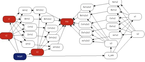
The network for one trace and a single marker follows Mortera et al. (2003), Fig. 4 section 3.2, an OOBN version considering up to three unknown contributors Fig. 6, marker network. Here we present the networks for the marker, FES4_.

Figure 6: marker network.

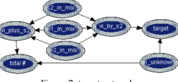
The instance target follows the reformulation of the query presented by Mortera et al. (2003) in order to use simple arithmetic expressions avoiding the tedious construction of the states and tables for the nodes; this is presented in more detail in Fig. 7.

4

The marker networks differ only in the number of alleles to consider, whether it is the space of states of the nodes referring the alleles or in the presence of one more allele to consider in the network. Since Hugin does not allow modification of the state of a node in order to reuse a network, for markers TH01 and FGA we started with a codification in the space of states of the node gene and put it in accordance with the alleles of each marker under consideration so that we could use the same network.

(12)

24

Figure 7: target network.

The node vi_plus_s2 takes values 0,1,2,3 according to the number of true states in its parent nodes v1_in_mix?, v2_in_mix? and s2_in_mix?. Consequently the node total# takes values from 0 to 6 being given by vi_plus_s2 + n_unknown. The node n_unknown accounts the number of possible unknown contributors to the mixture, between 0 and 3. Node vi_by_s2 takes values from 0 to 7, expressing the result values of the one-to-one correspondence with the eight joint configurations of its parent nodes v1_in_mix?, v2_in_mix? and s2_in_mix?. The target node has 32 states and is given by v_ by_s2 + 8 *n_ unknown. These 32 states of target node describe all the possibilities for contributors to the mixture, i.e., target has all states from v1&v2&s2&3u, v1&s2&3u,..., v1&v2&s2, ..., null. Naturally, the unrealistic hypotheses (those incompatible with the minimum number of contributors) are excluded when the evidence is inserted.

The nodes v1_in_mix?, v2_in_mix?, s2_in_mix?, target, vi_by_s2, and n unknown are given uniform prior distributions. The true or false states of the ui’s are indirectly given from the value of n_unknown and through the instance n_unk, Fig. 8. When n_ unknown is 0 then all the ui’s, in marker, are false, so none of this possible contributors is included in the mixture, when n_unknown = 1 then u1 is included in the mixture and similarly for states 2 and 3 of n_ unknown. This information is passed to the ui’s through n_unk and its respective nodes. Therefore, for example u1 is considered in the mixture when n_ unknown is more or equal to 1, i.e., n_unk >= 1 is true if n_ unknown is more or equal to 1 else is false. Similarly for u2 and u3.

Figure 9: n_unk network.

In the marker network we defined a new instance for each individual, Fig. 10.

(13)

For each person, v1, v2, s2, u1, u2, u3, we have a repeated structure in which we consider the genetic background information – the paternal and maternal inheritance, pg and mg. These are instances of a class named founder, a network constituted by a simple allele node in which the population allele frequencies are used to specify the unconditional distribution. By taking this approach we implement the product rule that is Hardy-Weinberg and linkage equilibrium assumptions. If a more complex genetic model was desired it could be implemented by introducing dependencies between founder nodes.

The individual’s genotype, known for v1, v2 and s2 and unknown for u1, u2 and u3, are indirectly inserted, for the known persons, through the instance allele_in shown in Fig. 11.

Figure 11: allele_in network.

The instances A, B, C and x5, instances of the class allele, Fig. 12, are expressing the logical conjunction between the query node and the presence or absence of the allele in the considered individual, given through allele_in. The node query represents a binary query mentioning if an individual (for example v1) is or is not in the mixture.

Figure 12: allele network.

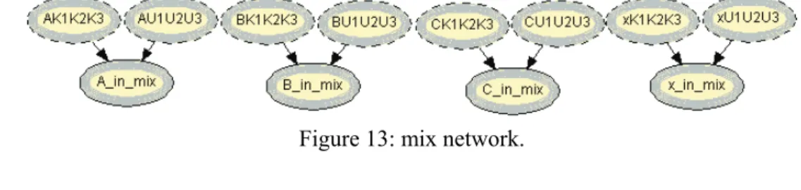
The instance marker has also an instance named mix, Fig. 13, which for each allele, expresses the logical disjunction of the parent instances, e.g., allele A is in the mixture if Av1v2s2 is true or Au1u2u3 is true. Here we use k to refer that the allele came from the known individual’s v1, v2 or s2, in the same way that u is used for the unknowns.

Figure 13: mix network.

5

For marker FES A, B and C (possibly translate to 8, 9, 11, etc) are the alleles present in the mixture and we use x to represent all the alleles not observed for the marker.

(14)

26

In marker the instances Av1v2, ..., xu1u2u3 are expressing the possession of an allele by at least one of the individuals v1, v2, s2, u1, u2, u3, instances of logical disjunction, Fig. 14, i.e, Av1v2 is true if at least one of v1 or v2 has allele A. The node vi_by_s2 is identical to the same named output node of the instance target, and it refers the probabilities of the state given the evidence. For each trace vi_by_s2 is the node measuring the presence of the suspect at the scene of the crime.

Figure 14: disjunction network.

We can put the network marker to run and obtain the results for one of the traces. 2.1.2 Two mixture traces and a single marker

In the case mentioned there were two different traces found at the scene of the crime. So it is necessary to combine the information from both traces. To do so we defined an instance combine, Fig. 15. This instance has as parents the output nodes vi_by_s2 of the instance marker for trace T1 and trace T2. The node T1_T2 combines the results obtained in the parent instances for node vi_by_s2 expressing the result values of the one-to-one correspondence with the eight joint configurations of its parent nodes v1_in_mix?, v2_in_mix?, s2_in_mix? in each trace (vi_by_s2_t1, vi_by_s2_t2) for the considered marker.

Figure 15: combine network.

Therefore, the node T1_T2 takes values 0, 1, 2, 3 corresponding to the hypothesis H4, H1, H2 and H3, respectively. T1_T2 is 0 if vi_by_s2 is less than 4 in T1 and T2; assumes value 1 if vi_by_s2 is equal to 4 or more in T1 and less than 4 in T2; takes value 2 if vi_by_s2 is less than 4 in T1 and equal to 4 or more in T2; and is 3 if vi_by_s2 is equal to 4 or more in both T1 and T2. We start with a uniform prior distribution for node T1_T2.

We are now able to put the networks for each trace together and compute the information in which we are interested, Fig. 16. The instances FES trace_t1 and FES trace_t2 are of class marker in which all the individuals in any of the networks have the same structure (individual). Its differentiation is made when the evidence is inserted.

(15)

Figure 16: combine_T1_T2 network.

When we combine the two traces in order to obtain a measure of the evidential weight associated with the possible presence of genetical material from the suspect in the traces found at the crime scene we get the results listed in the Tables below. For marker FES with different mixture traces we obtain: S2, V2, V1 trace T1 trace T2 0 (FFF) 0.0048 0.1470 1 (FFT) 0.1334 0.0000 2 (FTF) 0.0068 0.1791 3 (FTT) 0.1334 0.0000 4 (TFF) 0.0072 0.1881 5 (TFT) 0.3526 0.0000 6 (TTF) 0.0092 0.4857 7 (TTT) 0.3526 0.0000

Table 3: results of the node vi_by_s2

Where the state 0 corresponds to s2_in_mix? = False, v2_in_mix? =False and v1_in_mix? = False (FFF), and for simplicity the state 0 is read as S2; V2; V1 = FFF.

In Table 4 it is shown the combined information for the two traces for marker FES. H1 0.2353

H2 0.1876

H3 0.4862

H4 0.0908

Table 4: results for the node T1_T2. Thus,

(

S₂ contributedtoatleastoneof thetraces|ξ

)

=0.9092

P .

2.2 Generalizing two mixture traces and three markers

Given the results obtained for one marker it is necessary to extend the reasoning in order to consider the information for the three markers, FES, TH01 and FGA.

(16)

28

The instances combine_T1_T2 express the results for each marker accounting for the information

for the two traces. The node T1_T2 in each of these instances computes the results for each marker. Therefore we can extract the respective tables, similar to Table 4, for the other two markers.

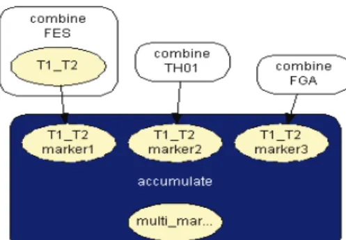
The instance accumulate having as inputs the output nodes of the instances combine T1_T2, with the results of each marker, incorporates the information for the two traces obtained separately, Fig. 17. The node multi_markers combines the information from the different instances combine_T1_T2, i.e., multi_markers gives the results synthesizing the results of T1_T2 for the three markers. The node multi_markers with states 0, 1, 2 and 3 assumes the state 0 if all the input nodes are 0. Takes value 1 if all the input nodes are 1 or at least one of the input nodes has state 1 and the others have the state 06. The node multi markers is 2 if all the input nodes have state 2 or this state 2 is combined between the states 0 and 2 of the input nodes. The node assumes state 3 if all the input nodes have state 3 or if the inputs are combining state 0, state 1 and state 2.

Figure 17: accumulate network.

When we join the networks for the three markers, each of which accounts for the two traces, we obtain the accumulate_three_markers network, Fig. 19.

Figure 19: accumulate three markers network.

Tables 5 and 6 display the results for the marker FGA and TH01 and the cumulative result for all three markers, rescaled to sum up to 1. This aims at the question of interest.

S2, V2, V1 trace T1 trace T2 trace T1 trace T2

0 (FFF) 0.0010 0.0084 0.0134 0.0134

1 (FFT) 0.0150 0.0000 0.0342 0.0342

2 (FTF) 0.0037 0.0476 0.0342 0.0342

6

e.g., multi markers=1 if

T1_T2 =1 for marker1, marker2 and marker3; or T1_T2 =1 for marker1 and marker2 and

T1_T2 =0 for marker3; or T1_T2 =1 for marker1 and marker3 and T1_T2 =0 for marker2; or T1_T2 =1 for marker2 and marker3 and T1_T2 =0 for marker1; or T1_T2 =1 for marker1 and T1_T2 =0 for marker2 and marker3; or T1_T2 =1 for marker2 and T1_T2 =0 for

(17)

Aplimat – Journal of Applied Mathematics volume 2 (2009), number 3 29 3 (FTT) 0.0290 0.0000 0.0342 0.0342 4 (TFF) 0.0079 0.0977 0.0599 0.0599 5 (TFT) 0.4644 0.0000 0.2748 0.2748 6 (TTF) 0.0146 0.8463 0.2748 0.2748 7 (TTT) 0.4644 0.0000 0.2748 0.2748

Table 5: results for the eight configurations for markers FGA and TH01.

H1 0.002114

H2 0.001568

H3 0.996313

H4 0.000003

Table 6: results for the node T1_T2 for markers FGA and TH01. Therefore, we can say that,

(

S₂contributedtoatleastoneof thetraces|ξ

)

=0.999997

P

When all the information for the two traces on the three markers is taken into account we get a very significant value for the quantity in which we are interested.

3 Comments

The use of DNA evidence analysis is commonly accepted nowadays in all courts. However, the presentation, interpretation and evaluation of this type of evidence sometimes raise some problems. And we are still far from a total incorporation of this kind of evidence, although in some cases it has been decisive for the conviction or absolution of the individuals. This is already a good support for justice, specially in disputed paternity cases.

The statistical treatment of criminal evidence has raised new challenges to those that have to decide, in the basis of the presented results. Independently of the methodology used, the great difficulty inhabits in the interpretation of the evidence, which is summarized in a number – what does that value means?

In the most complex problems, as the mentioned ones, the use of Bayesian networks for the analysis and interpretation of the evidence can be of great help. In a Bayesian network the complex inter-relations between the variables are transformed into modular units.

This tool – whose use is everyday more common in different areas – supplies, as a support to the decision, a number. It does not give the decision; it is a decision support instrument. Consequently it is important that the legal system knows how to evaluate and interpret correctly the information contained in it. However, there is still much to do.

Acknowledgement

(18)

30

References

[1] COWELL, R. G.. DAWID, A. P., LAURITZEN, S. L., SPIEGELHALTER, D. J. (1999). Probabilistic expert systems. Springer, New York.

[2] DAWID, A. P., MORTERA, J., PASCALI, V. L., van BOXEL, D. W. (2002). Probabilistic expert systems for forensic inference from genetic markers. Scandinavian Journal of Statistics, 29, 577-595.

[3] EVETT, I. W., GILL, P. D., JACKSON, G., WHITAKER, J. CHAMPOD, C. (2002). Interpreting small quantities of DNA: the hierarchy of propositions and the use of Bayesian networks. Journal of Forensic Sciences, 47, 520-530.

[4] MORTERA, J. (2003). Analysis of DNA mixtures using probabilistic expert systems. In: Green, P. J., Hjort, N. L., Richardson, S. (Eds.), Highly Structured Stochastic Systems. Oxford University Press

[5] MORTERA, J., DAWID, A. P., LAURITZEN, S. L. (2003). Probabilistic expert systems for DNA mixture profiling. Theoretical Population Biology, 63, 191-205.

Current address

Marina Alexandra Pedro Andrade, Professor Auxiliar

ISCTE - Instituto Superior de Ciências do Trabalho e da Empresa UNIDE - Unidade de Investigação e Desenvolvimento Empresarial, Av. das Forças Armadas 1649-026 Lisboa (Lisbon, Portugal), Tel. +351 217 903 000

e-mail: marina.andrade@iscte.pt

Manuel Alberto Martins Ferreira, Professor Catedrático

ISCTE - Instituto Superior de Ciências do Trabalho e da Empresa UNIDE - Unidade de Investigação e Desenvolvimento Empresarial, Av. das Forças Armadas 1649-026 Lisboa (Lisbon, Portugal), Tel. +351 217 903 000