FiSCal PoliCy reSPonSiveneSS, PerSiSTenCe and diSCreTion

W O R K I N G PA P E R S E R I E S

N O 9 5 4 / O C T O B E R 2 0 0 8

FISCAL POLICY

RESPONSIVENESS,

PERSISTENCE

AND DISCRETION

W O R K I N G PA P E R S E R I E S

N O 9 5 4 / O C T O B E R 2 0 0 8

In 2008 all ECB publications feature a motif taken from the 10 banknote.

FISCAL POLICY RESPONSIVENESS,

PERSISTENCE AND DISCRETION

by António Afonso

_{, Luca Agnello}

and Davide Furceri

This paper can be downloaded without charge from http://www.ecb.europa.eu or from the Social Science Research Network electronic library at http://ssrn.com/abstract_id=1284926.

1 We are grateful to Jacopo Cimadomo, Javier Pérez, Ad Van Riet, Jürgen von Hagen, participants at an ECB seminar, and an anonymous referee for helpful comments and to Silvia Albrizio and Matthijs Lof for research assistance. Luca Agnello would like to thank the Fiscal Policies Division of the ECB for its hospitality. The opinions expressed herein are those of the authors and do not necessarily reflect those of the ECB or the Eurosystem. 2 European Central Bank, Directorate General Economics, Kaiserstraße 29, D-60311 Frankfurt am Main, Germany;

© European Central Bank, 2008

Address

Kaiserstrasse 29

60311 Frankfurt am Main, Germany

Postal address

Postfach 16 03 19

60066 Frankfurt am Main, Germany

Telephone

+49 69 1344 0

Website

http://www.ecb.europa.eu

Fax

+49 69 1344 6000

All rights reserved.

Any reproduction, publication and reprint in the form of a different publication, whether printed or produced electronically, in whole or in part, is permitted only with the explicit written authorisation of the ECB or the author(s).

The views expressed in this paper do not necessarily refl ect those of the European Central Bank.

Abstract 4

Non-technical summary 5

1 Introduction 7

2 Literature 9

3 Empirical strategy 13

3.1 Fiscal measures of responsiveness,

persistence and discretion 13

3.2 What matters for the fi scal measures? 14

4 Results and discussion 16

4.1 Quantitative estimates for responsiveness,

persistence and discretion 16

4.2 Determinants of the fi scal measures 18

4.3 Robustness analysis 23

5 Conclusion 25

References 26

Tables and fi gures 29

Appendices 39

European Central Bank Working Paper Series 44

Abstract

We decompose fiscal policy in three components: i) responsiveness, ii) persistence and iii) discretion. Using a sample of 132 countries, our results point out that fiscal policy tends to be more persistent than to respond to output conditions. We also found that while the effect of cross-country covariates is positive (negative) for discretion, it is negative (positive) for persistence thereby suggesting that countries with higher persistence have lower discretion and vice versa. In particular, while government size, country size and income have negative effects on the discretion component of fiscal policy, they tend to increase fiscal policy persistence.

Keywords: Fiscal Policy, Fiscal Volatility.

Non-technical summary

In the last decade, several studies in the economic literature have assessed fiscal policy characteristics. Most of these studies analyze the responsiveness of fiscal policy, that is, the response of fiscal policy to output. Other contributions analyze the extent to which fiscal discretion impacts on the macroeconomic environment with the final objective to solve the trade-off between the degree of fiscal discipline and the necessary flexibility to deal with automatic stabilizers. Interestingly, few empirical studies asses the relevance of a third fiscal policy characteristic: persistence. Generally speaking, fiscal persistence can be considered as a measure of the degree of dependence of current fiscal behaviour on its own past developments. We contribute to the literature by providing evidence that also accounts for this latter fiscal characteristic.

In particular, we extend the analysis of Fatás and Mihov (2003, 2006) in several ways: i) we also compute a measure of fiscal persistence, allowing to cross-check persistence and discretion; ii) the abovementioned three fiscal components are obtained both for government spending and revenue; iii) we analyse the determinants of all three fiscal components with a set of macroeconomic, political and institutional variables, and geographical variables; iv) finally we also use several datasets.

1. Introduction

In the last decade, several studies in the economic literature have assessed fiscal policy characteristics. Most of these studies analyze the responsiveness of fiscal policy, that is, the response of fiscal policy to output, in order to explore the effectiveness of automatic stabilizers. Other contributions analyze the extent to which fiscal discretion

impacts on the macroeconomic environment.

Interestingly, few empirical studies asses the relevance of a third fiscal policy characteristic: persistence. Generally speaking, fiscal persistence can be considered as a measure of the degree of dependence of current fiscal behaviour on its own past developments. We contribute to the literature by providing evidence that also accounts for this latter fiscal characteristic. In particular, the aim of this paper is to disentangle fiscal policy (both government spending and revenue) in three components: responsiveness, persistence and discretion, and to assess which variables make these components to vary across countries. Thus, compared to existing work on the literature, we provide a broader and more comprehensive approach to assess the behaviour of fiscal policy (in terms of responsiveness, persistence and discretion) and its determinants.

In particular, we extend the analysis of Fatás and Mihov (2003, 2006) in several ways: i) we also compute a measure of fiscal persistence, allowing to cross-check persistence and discretion; ii) the abovementioned three fiscal components are obtained both for government spending and revenue; iii) we analyse the determinants of all three fiscal components with a set of macroeconomic, political and institutional variables, and geographical variables; iv) finally we also use several datasets.

processes describing the behaviour of both government expenditures and revenues. Finally, we identify discretion as the part of government spending and revenue that does not correspond to systematic responses to output conditions and in past values of government spending and revenue, but is instead the consequence of exogenous political processes or extraordinary non-economic circumstances.

Our analysis covers a set of 132 developed and developing countries over the period 1980-2007, as well as data for EU-15 countries over the period 1970-2007. The main results of the paper can be summarized as follows: a) fiscal policy is a-cyclical in most of the countries in the sample (i.e. responsiveness is generally small and in most of the cases not statistically significant) while persistence is the dominant component; b) more interestingly, there exists a significant trade-off between persistence and discretion. Both for revenue and spending, persistence is negatively correlated to the discretion component thereby suggesting that countries with higher persistence have lower discretion. These findings are supported by the results of the second part of the analysis. In fact, we found that regressing both discretion and persistence estimates on a common set of explanatory variables, the sign of the coefficient associated to many of these cross-country covariates is opposite in the two regressions.

Moreover, we find that macro and political and institutional variables can not account for responsiveness, once regional dummies are considered.

presents and discusses the results. Section five concludes with the main findings, policy implications and suggestion for future works.

2. Literature

The existing related literature has usually analyzed two of three abovementioned components of fiscal policy. On the one hand, the responsiveness of fiscal policy to output, and on the other hand, the discretionary part of fiscal policy. These two issues have deserved great interest since both are crucial for output stabilization and, therefore, indirectly for growth and aggregate welfare1.

The issue of responsiveness of fiscal policy has received increasing attention from researchers both from a theoretical and empirical point of view.

From a theoretical point of view, standard Keynesian models imply that fiscal

From an empirical point of view, the evidence is quite mixed, varying across spending and revenues categories as well as across countries. For OECD countries, some research shows that spending is counter-cyclical (Gali, 1994), while others show no discernible pattern (e.g. Fiorito, 1997; Gavin and Perotti, 1997b). The differences in these results depend on the components of spending being measured. For example, Gali (1994) studies government consumption and investment in a simple cross-country regression for a sample of 22 OECD countries and finds that both taxes and government purchases seem to

1

Regarding the relationship between output volatility, growth and welfare, see, for example, Ramey and Ramey (1995), Epaulard and Pommeret (2003), Fatás and Mihov (2003, 2005, 2006), Barlevy (2004), Furceri (2007, 2008) and Imbs (2007).

by Barro (1979) imply that government will smooth both tax rate and government spending in recessions and increase in booms. At the other stream, tax-smoothing models inspired policy should be counter-cyclical, i.e. government spending (taxes) should rise (decrease)

be effectively working as "automatic stabilizers", with government purchases following a counter-cyclical pattern. Fiorito and Kollintzas (1994) and Fiorito (1997), on the other hand, study specifically government consumption in the G-7 countries and find that the expenditures are either counter-cyclical or a-cyclical.

The limited number of empirical studies for developing countries suggests that government spending tends to be pro-cyclical. For example, Gavin and Perotti (1997a) find that fiscal policy is highly pro-cyclical in Latin America; Kaminsky, Reinhart, and Vegh (2004) find that fiscal policy is pro-cyclical in their sub-sample of 83 low- and middle-income countries; Braun (2001) finds that government expenditure is pro-cyclical in a panel of 35 developing countries for the period 1970-1998.

The conventional wisdom that emerges from these studies is that fiscal policy is counter-cyclical or a-cyclical in most developed countries, while it is pro-cyclical in developing countries. This result is corroborated by Lane (2003) who finds that the capability to implement fiscal control procedures is positively correlated with the level of development (measured by output per capita). This implies that richer countries enjoy less pro-cyclical government spending.

Several explanations have been advanced to explain the cross-country variation in the degree of fiscal cyclicality especially between developing and industrial countries.

appears to be broadly consistent with Barro’s tax smoothing proposition, in developing countries government spending and taxes are highly pro-cyclical.

Persson (2001), Persson and Tabellini (2001), Alesina and Tabellini (2005), also find that political and institutional factors matter also for fiscal responsiveness. In particular, while Persson (2001) and Persson and Tabellini (2001) find that parliamentary and majority based systems are related to cyclicality of fiscal policy, Alesina and Tabellini (2005) show that most of the pro-cyclicality of fiscal policy in developing countries can be explained by high levels of corruption.

Hallerberg and Strauch (2002) argue that fiscal policy is less anti-cyclical in the Economic and Monetary Union (EMU) countries in election years. Similar results in U.S. states are documented by Sorensen, Wu and Yosha (2001). Using data for OECD countries, Lane (2003) shows that countries with volatile output and dispersed political power are the most likely to run pro-cyclical fiscal policies.

Finally, an interesting contribution is the work of Galì and Perotti (2003). After estimating fiscal policy rules for eleven EMU countries over the period 1980-2002, they test whether fiscal constraints of the EMU – as embedded in the Maastricht Treaty and the Stability Growth Path – may be conducive of pro-cyclical fiscal policies. According to their results, anti-cyclical policies became stronger after the adoption of the Maastricht Treaty. Galì (2005) demonstrates that this latter evidence holds in general for all industrialized countries. Afonso (2008) also finds evidence of counter-cyclical responses of fiscal policy for the EU countries.

political and institutional determinants of discretionary fiscal policy and their effects on output volatility and economic growth. They use the term discretionary to refer to changes in fiscal positions that represent neither automatic reaction to economic conditions nor can be related to persistent changes in budget items. Using data from 91 countries, they find that highly volatile discretionary fiscal policy exerts a strong destabilizing effect on the economy. Additionally, fiscal policy is explained to a large extent by such variables as the characteristics of electoral and political systems and the lack of political constraints. They conclude that institutional arrangements that constrain discretion via checks and balances allow nations to achieve higher rates of economic growth and reduce macroeconomic instability.

More recently, Fatás and Mihov (2006), using data from 48 US states, explore the role that “rules” and institutions play in determining discretionary fiscal policy and look at whether the same rules and institutions influence the cyclicality of fiscal policy. Cyclicality is defined as the elasticity of government spending with respect to output. They find that strict budgetary restrictions lead to lower policy volatility and reduce the responsiveness of fiscal policy to output shocks. These two results should have opposite effects on output volatility. While less discretion should reduce volatility, less responsiveness of fiscal policy might amplify business cycles.

3. Empirical Strategy

3.1 Fiscal Measures of Responsiveness, Persistence and Discretion

Following Fatás and Mihov (2003, 2006), in order to differentiate between persistence, responsiveness and discretion in government spending and revenue we estimate for each country i (with i =1,…,N ) the following regressions:

t i t i G i t i G i t i G i G i t

i Y G

G_, log _, log _{, 1 , ,}

log D E J į Z H (1)

log R_i,t D_iR E_iR logY_i,t J_iR log

where G is real government spending, R is real government revenue, Y is real GDP, and Z

is a set of controls including also time trend2.

The estimates of the country-specific coefficients Ei, Jiand Vi in (1) and in (2)

(where Vi is the standard deviation of the residuals of the above regressions) will represent

respectively our measures of responsiveness, persistence, and a quantitative estimate of discretionary fiscal policy. In order to get these estimates, we include as control variables (i.e. the vector Zi) the current and the lagged value of real oil prices, the current inflation

rate and a linear time trend. Oil prices are included since they affect the state of the economy and more importantly because they contribute significantly to total revenue for some of the countries in the sample. We include inflation to ensure that our results are not driven by high inflation episodes. We also consider a time trend in our specifications, since government spending and revenue can also have a deterministic time trend in addition to the stochastic one. Finally, in order to control for possible endogeneity we use past values of real GDP as instruments.

2

3.2 What Matters for the Fiscal Measures?

Once we obtain the estimates for responsiveness (Eˆ_iG,R), persistence (Jˆ_iG,R) and

discretion (Vˆ_iG,R) of fiscal policy we can explain cross-country variation in fiscal policy

behaviour, regressing those estimates on a set of explanatory variables that the literature has found to be related to fiscal policy.

We estimate the following three cross-country equations (six considering both estimations for the spending and the revenue equation):

¦

¦

¦

j j ij j j ij j j ij i

R G

i D G D I P T E [

V_ˆ , ₁

log (3)

¦

¦

¦

j j ij j j ij j j ij i

R G

i D G D I P T E X

J_ˆ , ₂

(4)

¦

¦

¦

j j ij j j ij j j ij i

R G

i D G D I P T E Z

E_ˆ , ₃

(5)

for i = 1,…, N and where: Ej denotes macroeconomic variables; Pj denotes political and

institutional variables; Dj denotes demographic and geographical variables; ZQand [ are

well-behaved residuals; Į’s are nuisance coefficients; G, I, and T are our coefficients of

interest.

In more detail, the set of controls consists of the following variables:3

i) Macroeconomic variables (E): a) GDP per capita; b) openness; c) GDP deflator-based inflation rate; d) government size, and e) country size .4

ii) Political and institutional variables (P): a) an index of the level of democracy; b) an index for political stability; c) an index for presidential versus parliamentary electoral

3

See Appendix 1 for a detailed description of the variables and sources.

4

system, d) an index that accounts for constitutional limits on the number of years the executive can serve before new elections; e) an index of government effectiveness; f) the Herfindahl index of parties concentration in the government, g) a dummy if the chief executive is a military chief.5

iii) Geographical variables (D)6: a) the log of absolute latitude (kilometres from the equator); b) regional dummies for developing countries from b1) Latin America, b2) Sub-Saharan Africa, b3) East Asia, b4) South Asia, b5) Europe-Central Asia, b6) and Middle East-North Africa.7

Since our dependent variables are based on estimates, the regression residuals can be thought of as having two components. The first component is sampling error (the difference between the true value of the dependent variable and its estimated value). The second component is the random shock that would have been obtained even if the dependent variable was directly observed as opposed to estimated. This would lead to an increase in the standard deviation of the estimates, which would lower the t-statistics. This means that any correction to the presence of this un-measurable error term will increase the significance of our estimates8.

We estimate equations (4)-(5) by Weighted Least Squares (WLS). This choice takes account of the fact that the dependent variables are measured with different degrees

5

The economic literature has generally focused on political and institutional characteristics to explain cross country differences in government spending (Drazen, 2000; Persson, 2001; Persson and Tabellini, 2001). See Fatás and Mihov (2003) for a more detailed discussion.

6

Alesina and Wacziarg (1998) have found that geographical variables are important to explain cross country differences in government spending.

7

As suggested by La Porta et al. (1999), it is likely that latitude from the equator, income and regional dummies are related to the quality of government and institutions.

8

of precision across countries, and of the fact that some of the estimated values of our dependent variables are not statistically significant from zero.9

4. Results and discussion

We use data from the IMF World Economic Outlook for a set of 132 countries for which we have data available from 1980 to 2007 (see the data Appendix for further details).10 Moreover, using data from the European Commission AMECO database, we perform a similar exercise for the 15 “old” members of the European Union (EU-15), for which the time sample broadly spans between 1960 and 2007.

4.1 Quantitative Estimates for Responsiveness, Persistence and Discretion

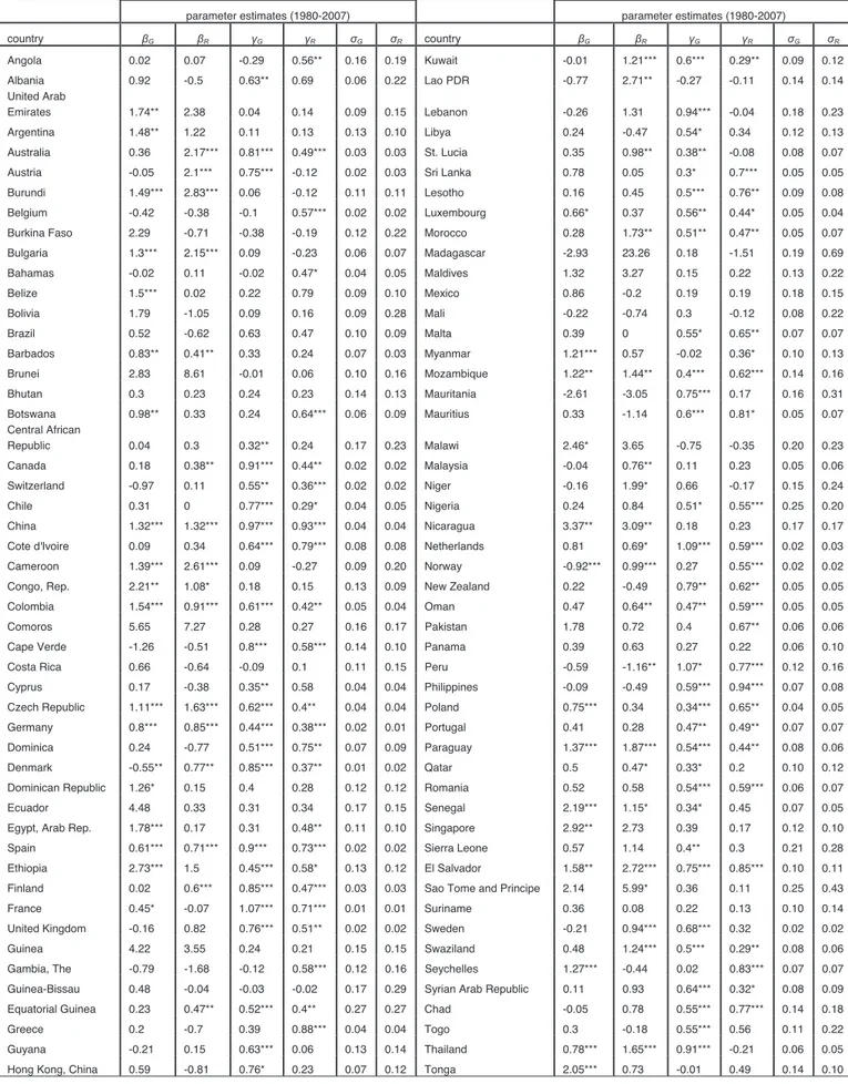
We start our empirical analysis by estimating the coefficients of responsiveness, discretion and persistence. The results relative to both government spending and revenue, for the entire set of countries are reported in Table 1. Looking at the table it is possible to see that in terms of magnitude the coefficient of persistence in the great majority of the cases is bigger than the one of responsiveness. This is also confirmed by the fact, that while the coefficient of persistency is statistically significant in most of the cases (73 times for spending and 68 times for revenue) the coefficient used as our measure of fiscal responsiveness is statistically significant for a smaller number of cases (42 times for spending and 48 for revenue). Thus, it seems that overall, fiscal policy tends to be more persistent than to respond to current output conditions. Moreover, it is interesting to note that while government revenue reacts relatively more to output than government spending, spending overall seems to be more persistent than revenue.

9

See, Lane (2003) for a similar approach. All the results presented do not qualitatively change when we estimate equations (3)-(5) by OLS.

10

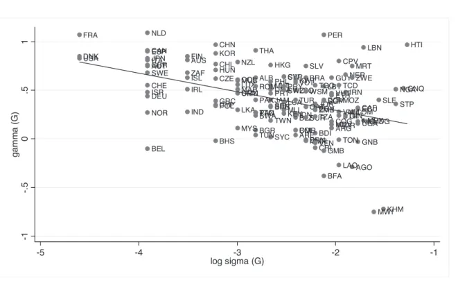
We remark thatour discretion estimates are computed as the standard deviation of the residuals from both government spending and revenue equations. Thus, it is clear that the lower and less significant are the coefficients of responsiveness and persistence the higher will be the component of discretion11. This argument, together with the fact that fiscal policy seems to be more persistent than responsive, suggests a negative relation between the measures of persistence and discretion. This intuition is empirically confirmed. Figure 1 provides the scatter plot of our measures of persistence against discretion exhibiting a negative relation between these two variables. In particular, the estimate of this simple bivariate relation for the spending equation is:

) 39 . 5 ( ) 89 . 0 ( ˆ log 190 . 0 09 . 0 ˆ G i G i V J

with R2 = 0.18 (t statistics are in parenthesis). The negative relationship also holds for the revenue equation (see Figure 2):12

) 16 . 4 ( ) 01 . 0 ( ˆ log 143 . 0 00 . 0 ˆ R i R i V J

with R2 = 0.12 (t statistics are in parenthesis). Thus, it seems that countries with higher persistence have a lower discretionary component of fiscal policy. In Table 2 we also report a rank analysis for our measure of persistence and discretion.

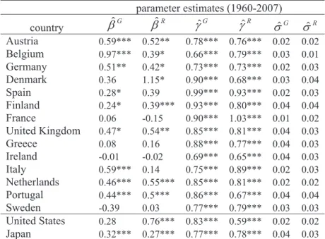
In order to check for the robustness of our results, we consider another data source for both revenues and government spending: the AMECO dataset comprising data from 1960 to 2007 for European Union countries. Therefore, we have considered the “old” EU-15 countries, with exception of Luxemburg, for which data are not available for the period

11 In fact, the lower the significance of the coefficients, the lower the R-squared of the regression, and the higher the variance of the residuals.

12

The correlation between Jˆ_iG and lnVˆ_iG equals to -0.43 while the correlation between Jˆ_iR and lnVˆ_iR

1988-89. For comparative purposes, we have decided to include also the United States and Japan.

Table 3 reports parameter estimates of responsiveness, persistence and discretion from the equations (1)-(2) over the sample period 1960-2007. We note that, while

parameter estimates G i

Jˆ and R i

Jˆ are always statistically significant (at 1% for all countries),

estimates ofE s are significant only for 62% of the cases (10 countries out of 16 for both

revenues and spending). Moreover, we also find a negative correlation betweenJ

coefficients and their corresponding discretionary components. In particular, we find that

the cross-country correlation betweenJˆ and _iG G i

Vˆ

log equals -0.14 while the cross-country

correlation between Jˆ and _iR R i

Vˆ

log is -0.32.

The above results corroborate our previous conclusions: a) persistence is the dominant component of both government spending and revenue while evidence about their responsiveness to the economic conditions is less clear; b) there is a negative relationship between the degree of persistence and discretion.

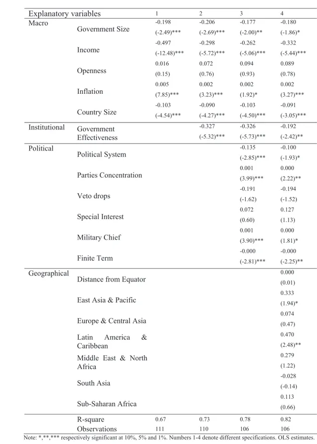
4.2 Determinants of the Fiscal Measures

In the previous section we found a significant and negative relation between discretion and persistence. On the one hand, this is partly explained by the fact that fiscal policy is not responsive for many countries in our sample. On the other hand, these results can be explained by the fact that if spending is left to discretionary actions and political decision its development will be less persistent, deviating more from the trend.

specification for our measures of persistence and discretion. In other words we expect that (at least for some variables) if a cross-country covariate has a negative (positive) impact on discretion it should have a positive (negative) impact on persistence.

In the second column of Table 4 we present the results obtained when institutional variables are taken into account. While the macroeconomic variables continue to be significant, we find that also government effectiveness is significantly and negatively related to discretionary spending. This is in line with previous results in the literature (Persson and Tabellini, 2001; Fatás and Mihov, 2003). Moreover, we find that considering alternatively different proxies for the quality of institutions (voice and accountability; political stability; regulatory quality; rule of law; and control of corruption) the results are almost unchanged (due to the high correlation among these indicators)13.

In the third column of Table 4, we show the results when political variables are also included. We can see that the political system proxy variables, parties’ concentration, the dummy for military chief and for the presence for a finite term are also related to our discretion measure. In particular, in line with Persson and Tabellini (2001), we find that the presidential system is associated with more discretionary spending, since in a parliamentary system the executive is supported by the parties in the parliament and therefore is constrained in the implementation of policy by the threat of a no-confidence vote. In a presidential system the president does not face the confidence requirement and hence can alter more easily policy either for opportunistic or partisan reasons. Therefore, presidential regimes may be associated with more volatile discretionary policy.

We also find that a lower concentration (lower Herfindahl index) in the government leads to higher discretion, since proportional systems lead to coalitions and fiscal deadlocks which delay stabilizations and increase discretionary spending (as argued by Alesina and Perotti, 1994).

assumes 1 if this is the case) tends to result in the use of fiscal policy in a more activist way. The results are robust when we include geographical and regional variables.

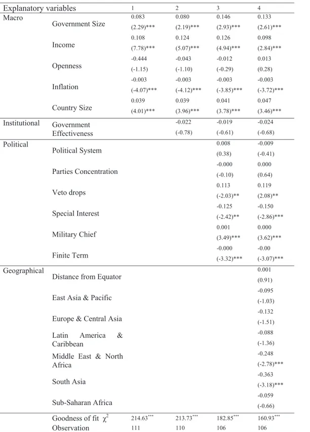
We now proceed to analyze the determinants for persistence of government spending. In Table 5 we report the results of estimating equation 4. In particular, as we did for the estimate of our discretion equation, we report four columns each presenting a different specification of the set of controls.

As already argued, we should expect at least for some of the controls, that if a cross country covariate has a negative (positive) impact on discretion it should have a positive (negative) impact on the persistence of government spending. This intuition is confirmed by our results. In fact, looking at the first column of Table 5, we can see that most of the macroeconomic variables are statistically significant and they have opposite signs with respect to the volatility of spending discretion.

However there are exceptions. For example, institutional variables are not significant in the specification for fiscal persistence but they are significant in the fiscal discretion specification. Other variables such as military chief and finite term enter with the same sign in both the persistence and the discretionary equation. In particular, we find that countries with higher political stability and with a military chief have a more persistent government spending. In contrast, countries where the executive has a given finite term or in which the executive represent special interests have a less persistent government spending.

components of discretion and persistence of government revenue are affected in a similar way by our set of explanatory variables cannot be taken for granted.

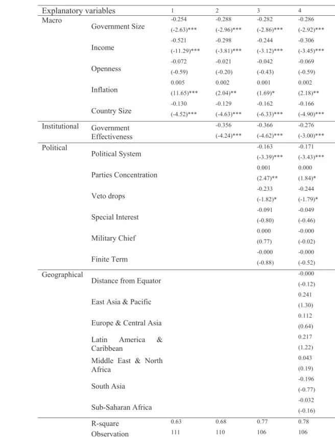
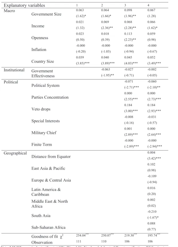
In Table 6 and 7, we report the estimates of equations (3) and (4) for government revenue. Focusing first on the revenue discretion equation (Table 6), we can observe that similarly to the volatility of government spending discretion, government size, country size, income, government effectiveness, parliamentary system and veto drops are negatively associated with the discretion component of revenue. In contrast, countries with higher inflation and characterized by lower concentration of parties tend to have more government revenue discretion.

Analyzing the results for revenue persistence (Table 7) we can see that, as for the spending specification, macroeconomic variables such as income and country size are significant and they have opposite sign with respect to the revenue discretion equation. In contrast, government effectiveness, political stability, parliamentary system and party concentration have the same sign in both the persistence and discretion equation (Tables 6 and 7). Other variables such as military chief and finite term are only significant in the persistence specification, and the sign of their coefficients is the same as in the spending specification.

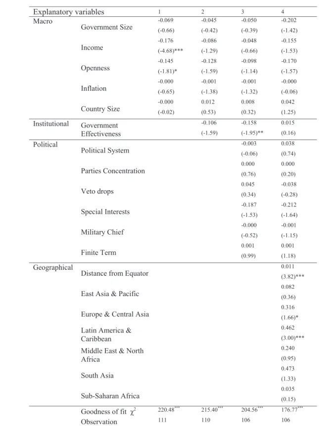
statically significant. In contrast, as argued by Gavin and Perotti (1997a), we find that government spending is highly pro-cyclical in Latin America.

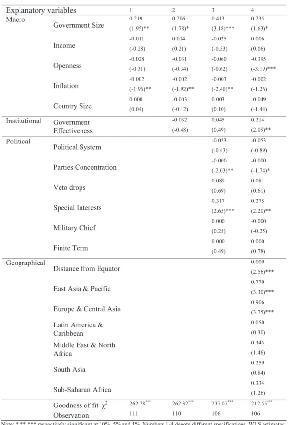
Different results are obtained when we estimate equation (5) for government revenue (Table 9). In particular, we find that while government size, government effectiveness, special interests, East Asia & Pacific, and Europe & Central Asia dummies are positively associated with revenue responsiveness, openness is negatively related. This different behaviour between the responsiveness of government spending and revenue is coherent with the fact that countries with pro-cyclical (counter-cyclical) spending may not have necessarily pro-cyclical (counter-cyclical) revenue, and vice versa.

4.3 Robustness Analysis

The behaviour of fiscal policy varies across countries.Thus, it is interesting to see whether our estimated measures of responsiveness, persistence and discretion are different across groups of countries. To this purpose, we consider three groups of countries: EMU, OECD and non OECD countries. Looking at the panel results reported in Table 10, it is possible to see that the responsiveness of both expenditure and revenue to output is lower than for the measure of persistence for all set of countries. Moreover, it does not seem that countries significantly differ in terms of responsiveness. In contrast, country groups systematically differ in terms of discretion and persistence of both expenditure and revenue. In particular, EMU countries are those characterized by the lowest estimated discretion coefficient for spending, while non OECD countries are those with the highest (lowest) level of discretion (persistence).

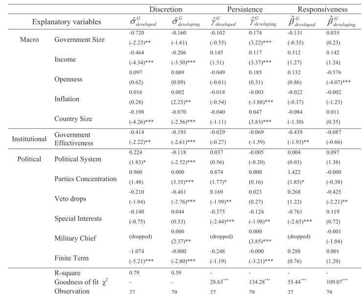
and developing countries. Thus, both from a theoretical perspective and, especially, from a policy point of view it is important to assess whether our analysis is robust within developed and developing country grouping. Table 11 reports the results both for the discretion, persistence and responsiveness equations for government spending. The first two columns refer to the results relative to fiscal discretion respectively for developed and developing countries. Looking at these two columns, it seems that there is not much discrepancy between the two groups. For both sets of countries, spending discretion is negatively related to GDP per capita, country size, government effectiveness and the dummy for finite terms. In contrast, other political variables and inflation seem to affect spending discretion only for developing countries.

The second two columns report the results of the persistence equation for both developed and developing countries. Differently from what was obtained for the equation regarding the discretion component, it seems that while macroeconomic variables have been more relevant for fiscal persistence in developing countries, political and institutional variables in general played a role in affecting fiscal persistence in both developed and developing countries, even if with some differences.

Finally, analyzing the last two columns we can see that the determinants of responsiveness of government spending vary between developed and developing countries. In particular, while government effectiveness and special interests are essentially the only variables found to be significant in the specification for developed countries, openness and veto drops are the only variables that have a statistically significant impact on spending responsiveness in developing countries. This result suggests that not only the measure of responsiveness and cyclicality varies between developing and developed countries, but this is also true for its determinants.

5. Conclusion

By making use of a two-step estimation procedure, we pursue a twofold objective in this paper. First, we provide an empirical study on the decomposition of fiscal policy into three components: responsiveness, persistence and discretion. Second, we analyze the determinants of these components. The key conclusions of our analysis are as follows.

Using a country-specific estimation approach to disentangle the abovementioned three components of fiscal policy, both for government spending and revenue, we find that, for most of the 132 countries in our sample, fiscal policy is rather more persistent than responsive to current economic conditions. More interestingly, we find that, for both revenue and spending, persistence is negatively correlated to the discretion component thereby suggesting that countries with higher persistence have lower discretion. The above conclusions are robust by considering the AMECO dataset for EU countries, for a larger time span. In the second part of our analysis, we carry out a cross-country estimation approach to identify the source of fluctuations of persistence, responsiveness and discretion components. According to the previous empirical finding, suggesting a negative relationship between discretion and persistence, we find that while government size and effectiveness and income have negative effects on the discretion component of fiscal policy, they tend to increase fiscal persistence. Moreover, we find that macro and political and institutional variables are less relevant for responsiveness, once regional dummies are considered.

Afonso, A. (2005). “Fiscal Sustainability: the Unpleasant European Case”, FinanzArchiv, 61 (1), 19-44.

Afonso, A. (2008). “Ricardian Fiscal Regimes in the European Union”, Empirica, 35 (3), 313–334.

Afonso, A. and Rault, C. (2007). “What do we really know about fiscal sustainability in the EU? A panel data diagnostic”, ECB Working Paper n. 820.

Akitoby, B., Clements, B., Gupta S., and Inchauste, G. (2004). “The cyclical and long-term behavior of government expenditures in developing countries”, IMF Working Paper 04.202.

Alesina, A., Campante, F. and Tabellini, G. (2008). “Why is Fiscal Policy Often Procyclical?” Journal of the European Economic Association, 6(5), forthcoming.

Alesina, A. and Perotti, R. (1994). “The Political Economy of Budget Deficits”, NBER Working Paper 4637.

Alesina A. and Tabellini G. (2005). “Why is fiscal policy often procyclical?” mimeo, July. Alesina, A. and Wacziarg, R. (1998). “Openness, country size and government”, Journal

of Public Economics,69 (3), 305-321.

Barlevy G. (2004). “The Cost of Business Cycles and the Benefits of Stabilization: A Survey”, NBER Working Paper 10926.

Barro R. (1979). “On the Determination of the Public Debt”, Journal of Political Economy, 87 (5), 93-110.

Braun M. (2001). “Why Is Fiscal Policy Procyclical in Developing Countries”, Harvard University.

Darby, J. and Melitz, J. (2007). “Labour Market Adjustment, Social Spending and the Automatic Stabilizers in the OECD”, CEPR Discussion Paper 6230.

Drazen, A. (2000). Political Economy in Macroeconomics, Princeton: Princeton University Press.

Epaulard, A. and Pommeret, A. (2003). “Recursive Utility, Endogenous Growth, and the Welfare Cost of Volatility”, Review of Economic Dynamics, 6(3), 672-684.

Fatás, A. and Mihov, I. (2001). “Government Size and Automatic Stabilizers”, Journal of International Economics, 55, 3-28.

Fatás, A. and Mihov, I. (2006). “The Macroeconomics Effects of Fiscal Rules in the US States”, Journal of Public Economics, 90, 101-117.

Ferejohn. (1986). “Incumbent performance and electoral control”, Public Choice 30, 5-25. Fiorito R. (1997). “Stylized Facts of Government Finance in the G-7”, IMF Working

Paper 97/142.

Fiorito R. and Kollintzas T. (1994). “Stylized Facts of Business Cycles in the G7 from a Real Business Cycles Perspective”, European Economic Review, Vol. 38, pp. 235-69. Furceri, D. (2007). “Is Government Expenditure Volatility Harmful for Growth? A

Cross-country Analysis”, Fiscal Studies, 28 (1), 103-120.

Furceri, D., and Poplawski, M. (2008). “Fiscal Volatility and the size of Nations”, Mimeo. Gali J. (1994). “Government Size and Macroeconomic Stability”, European Economic

Review, 38 (1), 117-32.

Galí J. (2005). “Modern perspective of fiscal stabilization policies”, CESifo Economic Studies, 51 (4), 587-599.

Galí J. and Perotti R. (2003). “Fiscal policy and monetary integration in Europe”, Fiscal Policy, 533-572 (October).

Gavin M. and Perotti R. (1997a). “Fiscal policy in Latin America”, NBER Macroeconomics Annual, (12), 11-71.

Gavin M. and Perotti R. (1997b). “Fiscal policy and saving in good times and bad times”, in Hausman R., Reisen H. (Eds.), Promoting Savings in Latin America, IDB and OECD.

Hallerberg, M. and Strauch, R. (2002). “On the Cyclicality of Fiscal Policy in Europe”,

Empirica, 29, 183-207.

Imbs, J. (2007). “Growth and volatility”, Journal of Monetary Economics, 54 (7), 1848-1862.

Kaminsky, G., Reinhart, C. and Végh, C. (2004). “When It Rains, It Pours: Procyclical Capital Flows and Macroeconomic Policies”, NBER Working Paper 10780.

Lane, P. (2003). “The cyclical behaviour of fiscal policy: evidence from the OECD”,

Journal of Public Economics, 87 (12), 2261-2675.

La Porta, R., Lopez de Silanes, F., Shleifer, A. and Vishny, R. (1998). “The Quality of Government”, Journal of Law, Economics and Organization, 15 (1), 222-279.

Persson, T. and Tabellini, G. (2001). “Political Institutions and Policy Outcomes: What are the Stylized Facts ? ” CEPR Discussion Papers 2872.

Ramey and Ramey (1995). “Cross-Country Evidence on the Link between Volatility and Growth”, American Economic Review, 85 (5), 1138-51.

Rand, J., and Tarp, F. (2002). “Business cycles in developing countries: Are they different?” World Development, 30 (12), 2071-2088.

Rodrick, D. (1998). “Why Do More Open Economies Have Bigger Governments?”

Journal of Political Economy, 106 (5), 997-1032.

Sorensen, B., Wu, L. and Yosha, O. (2001). “Output fluctuations and fiscal policy: U.S. state and local governments 1978–1994”, European Economic Review, 45, 1271-310. Talvi E. and Vegh, C. (2005). “Tax base variability and procyclical fiscal policy”, Journal

of Economic Development, 78 (1), 156-190.

Figure 1. Scatter plot ofJˆ vs._iG G i

Vˆ from country-specific spending equation.

AGO ALB ARE ARG AUS AUT BDI BEL BFA BGR BHS BLZ BOL BRA BRB BRN BTN BWA CAF CAN CHE CHL CHN CIV CMR COG COL COM CPV CRI CYP CZE DEU DMA DNK DOM ECU EGY ESP ETH FIN FRA GBR GIN GMB GNB GNQ GRC GUY HKG HTI HUN IDN IND IRL _IRN ISL ISR ITA JAM JOR JPN KEN KHM KIR KOR KWT LAO LBN LBY LCA LKA LSO LUX MAR MDG MDV MEX MLI MLT MMR MOZ MRT MUS MWI MYS NER NGA NIC NLD NOR NZL OMN PAK PAN PER PHL POL PRTPRY QAT ROM

SEN SGP SLE

SLV STP SUR SWE SWZ SYC SYR TCD TGO THA TON TTO TUN TUR

TWN TZA _UGA

URY USA VCT VEN VNM VUT WSM ZAF ZMB ZWE -1 -. 5 0 .5 1 gam m a (G)

-5 -4 -3 -2 -1

log sigma (G)

Figure 2. Scatter plot of Jˆ vs._iR R i

Vˆ from country-specific revenue equation.

AGO ALB ARE ARG AUS AUT BDI BEL BFA BGR BHS BLZ BOL BRA BRB BRN BTN BWA CAF CAN CHE CHL CHN CIV CMR COG COL COM CPV CRI CYP CZE DEU DMA DNK DOMECU EGY ESP ETH FIN FRA GBR GIN GMB GNB GNQ GRC GUY HKG HTI HUN IDN IND IRL IRN ISL ISR ITA JAM JOR JPN KEN KHM KIR KOR KWT LAO LBN LBY LCA LKA LSO LUX MAR MDG MDV MEX MLI MLT MMR MOZ MRT MUS MWI MYS NER NGA NIC NLD

NOR NZLOMN

PAK PAN PER PHL POL PRT PRY QAT ROM SEN SGP SLE SLV STP SUR SWE _SWZ SYC SYR TCD TGO THA TON TTO TUN TUR TWN TZA UGA URY USA VCT VEN VNM VUTWSM ZAF ZMB ZWE -1 .5 -1 -. 5 0 .5 1 ga m m a ( R )

Table 1. Estimates of Responsiveness (E), Persistence (J) and Discretion (V)

parameter estimates (1980-2007) parameter estimates (1980-2007)

country ȕG ȕR ȖG ȖR ıG ıR country ȕG ȕR ȖG ȖR ıG ıR

Angola 0.02 0.07 -0.29 0.56** 0.16 0.19 Kuwait -0.01 1.21*** 0.6*** 0.29** 0.09 0.12 Albania 0.92 -0.5 0.63** 0.69 0.06 0.22 Lao PDR -0.77 2.71** -0.27 -0.11 0.14 0.14

United Arab

Emirates 1.74** 2.38 0.04 0.14 0.09 0.15 Lebanon -0.26 1.31 0.94*** -0.04 0.18 0.23 Argentina 1.48** 1.22 0.11 0.13 0.13 0.10 Libya 0.24 -0.47 0.54* 0.34 0.12 0.13 Australia 0.36 2.17*** 0.81*** 0.49*** 0.03 0.03 St. Lucia 0.35 0.98** 0.38** -0.08 0.08 0.07

Austria -0.05 2.1*** 0.75*** -0.12 0.02 0.03 Sri Lanka 0.78 0.05 0.3* 0.7*** 0.05 0.05 Burundi 1.49*** 2.83*** 0.06 -0.12 0.11 0.11 Lesotho 0.16 0.45 0.5*** 0.76** 0.09 0.08 Belgium -0.42 -0.38 -0.1 0.57*** 0.02 0.02 Luxembourg 0.66* 0.37 0.56** 0.44* 0.05 0.04 Burkina Faso 2.29 -0.71 -0.38 -0.19 0.12 0.22 Morocco 0.28 1.73** 0.51** 0.47** 0.05 0.07 Bulgaria 1.3*** 2.15*** 0.09 -0.23 0.06 0.07 Madagascar -2.93 23.26 0.18 -1.51 0.19 0.69 Bahamas -0.02 0.11 -0.02 0.47* 0.04 0.05 Maldives 1.32 3.27 0.15 0.22 0.13 0.22

Belize 1.5*** 0.02 0.22 0.79 0.09 0.10 Mexico 0.86 -0.2 0.19 0.19 0.18 0.15 Bolivia 1.79 -1.05 0.09 0.16 0.09 0.28 Mali -0.22 -0.74 0.3 -0.12 0.08 0.22

Brazil 0.52 -0.62 0.63 0.47 0.10 0.09 Malta 0.39 0 0.55* 0.65** 0.07 0.07 Barbados 0.83** 0.41** 0.33 0.24 0.07 0.03 Myanmar 1.21*** 0.57 -0.02 0.36* 0.10 0.13

Brunei 2.83 8.61 -0.01 0.06 0.10 0.16 Mozambique 1.22** 1.44** 0.4*** 0.62*** 0.14 0.16 Bhutan 0.3 0.23 0.24 0.23 0.14 0.13 Mauritania -2.61 -3.05 0.75*** 0.17 0.16 0.31

Botswana 0.98** 0.33 0.24 0.64*** 0.06 0.09 Mauritius 0.33 -1.14 0.6*** 0.81* 0.05 0.07 Central African

Republic 0.04 0.3 0.32** 0.24 0.17 0.23 Malawi 2.46* 3.65 -0.75 -0.35 0.20 0.23 Canada 0.18 0.38** 0.91*** 0.44** 0.02 0.02 Malaysia -0.04 0.76** 0.11 0.23 0.05 0.06 Switzerland -0.97 0.11 0.55** 0.36*** 0.02 0.02 Niger -0.16 1.99* 0.66 -0.17 0.15 0.24

Chile 0.31 0 0.77*** 0.29* 0.04 0.05 Nigeria 0.24 0.84 0.51* 0.55*** 0.25 0.20 China 1.32*** 1.32*** 0.97*** 0.93*** 0.04 0.04 Nicaragua 3.37** 3.09** 0.18 0.23 0.17 0.17

Cote d'Ivoire 0.09 0.34 0.64*** 0.79*** 0.08 0.08 Netherlands 0.81 0.69* 1.09*** 0.59*** 0.02 0.03 Cameroon 1.39*** 2.61*** 0.09 -0.27 0.09 0.20 Norway -0.92*** 0.99*** 0.27 0.55*** 0.02 0.02 Congo, Rep. 2.21** 1.08* 0.18 0.15 0.13 0.09 New Zealand 0.22 -0.49 0.79** 0.62** 0.05 0.05

Colombia 1.54*** 0.91*** 0.61*** 0.42** 0.05 0.04 Oman 0.47 0.64** 0.47** 0.59*** 0.05 0.05

Comoros 5.65 7.27 0.28 0.27 0.16 0.17 Pakistan 1.78 0.72 0.4 0.67** 0.06 0.06 Cape Verde -1.26 -0.51 0.8*** 0.58*** 0.14 0.10 Panama 0.39 0.63 0.27 0.22 0.06 0.10

Costa Rica 0.66 -0.64 -0.09 0.1 0.11 0.15 Peru -0.59 -1.16** 1.07* 0.77*** 0.12 0.16 Cyprus 0.17 -0.38 0.35** 0.58 0.04 0.04 Philippines -0.09 -0.49 0.59*** 0.94*** 0.07 0.08 Czech Republic 1.11*** 1.63*** 0.62*** 0.4** 0.04 0.04 Poland 0.75*** 0.34 0.34*** 0.65** 0.04 0.05 Germany 0.8*** 0.85*** 0.44*** 0.38*** 0.02 0.01 Portugal 0.41 0.28 0.47** 0.49** 0.07 0.07

Dominica 0.24 -0.77 0.51*** 0.75** 0.07 0.09 Paraguay 1.37*** 1.87*** 0.54*** 0.44** 0.08 0.06 Denmark -0.55** 0.77** 0.85*** 0.37** 0.01 0.02 Qatar 0.5 0.47* 0.33* 0.2 0.10 0.12 Dominican Republic 1.26* 0.15 0.4 0.28 0.12 0.12 Romania 0.52 0.58 0.54*** 0.59*** 0.06 0.07

Ecuador 4.48 0.33 0.31 0.34 0.17 0.15 Senegal 2.19*** 1.15* 0.34* 0.45 0.07 0.05 Egypt, Arab Rep. 1.78*** 0.17 0.31 0.48** 0.11 0.10 Singapore 2.92** 2.73 0.39 0.17 0.12 0.10

Spain 0.61*** 0.71*** 0.9*** 0.73*** 0.02 0.02 Sierra Leone 0.57 1.14 0.4** 0.3 0.21 0.28

Ethiopia 2.73*** 1.5 0.45*** 0.58* 0.13 0.12 El Salvador 1.58** 2.72*** 0.75*** 0.85*** 0.10 0.11 Finland 0.02 0.6*** 0.85*** 0.47*** 0.03 0.03 Sao Tome and Principe 2.14 5.99* 0.36 0.11 0.25 0.43

France 0.45* -0.07 1.07*** 0.71*** 0.01 0.01 Suriname 0.36 0.08 0.22 0.13 0.10 0.14 United Kingdom -0.16 0.82 0.76*** 0.51** 0.02 0.02 Sweden -0.21 0.94*** 0.68*** 0.32 0.02 0.02

Guinea 4.22 3.55 0.24 0.21 0.15 0.15 Swaziland 0.48 1.24*** 0.5*** 0.29** 0.08 0.06 Gambia, The -0.79 -1.68 -0.12 0.58*** 0.12 0.16 Seychelles 1.27*** -0.44 0.02 0.83*** 0.07 0.07

Guinea-Bissau 0.48 -0.04 -0.03 -0.02 0.17 0.29 Syrian Arab Republic 0.11 0.93 0.64*** 0.32* 0.08 0.09 Equatorial Guinea 0.23 0.47** 0.52*** 0.4** 0.27 0.27 Chad -0.05 0.78 0.55*** 0.77*** 0.14 0.18

Greece 0.2 -0.7 0.39 0.88*** 0.04 0.04 Togo 0.3 -0.18 0.55*** 0.56 0.11 0.22 Guyana -0.21 0.15 0.63*** 0.06 0.13 0.14 Thailand 0.78*** 1.65*** 0.91*** -0.21 0.06 0.05

Table 1 (contd.). Estimates of Responsiveness (E), Persistence (J) and Discretion (V)

parameter estimates (1980-2007) parameter estimates (1980-2007)

country ȕG ȕR ȖG ȖR ıG ıR country ȕG ȕR ȖG ȖR ıG ıR

Haiti -3.74 -5.82 0.97*** 0.93*** 0.28 0.36 Trinidad and Tobago 1.09*** 0.55** 0.27 0.27 0.06 0.06 Hungary 0.23 1.42*** 0.71*** 0.15 0.04 0.03 Tunisia 2.06 3.72 0.04 0.13 0.06 0.08

Indonesia 0 0.33 0.25 0.18 0.09 0.06 Turkey 0.06 0.28 0.4 0.14 0.09 0.08 India 1.23** 0.63** 0.28* -0.07 0.03 0.03 Taiwan 1.75* 1.38 0.19 -0.01 0.07 0.05 Ireland 0.26 0.31* 0.51*** 0.33* 0.03 0.03 Tanzania 0.95 0.85 0.23 0.04 0.11 0.09

Iran, Islamic Rep. 0.57 0.51 0.48** 0.64** 0.15 0.17 Uganda 1.28 2.02* 0.16 0.08 0.17 0.18 Iceland 0.56** 0.82*** 0.63*** 0.32** 0.03 0.03 Uruguay 0.84*** 1.05** 0.47** 0.41* 0.05 0.06 Israel 0.77*** 0.33 0.48*** 0.37* 0.02 0.05 United States 0.27 1.05*** 0.83*** 0.51** 0.01 0.03

Italy 1.15*** 0.68* 0.81*** 0.8*** 0.02 0.02 St. Vincent and the

Grenadines -0.07 -1.31 0.58* 0.59* 0.09 0.08 Jamaica -1.1 -1.24 0.4** 0.57** 0.07 0.10 Venezuela, RB 1.07 -0.29 -0.04 0.63 0.11 0.11 Jordan 0.42 0.07 0.36 0.24 0.11 0.09 Vietnam -1.15 -1.27 0.28 0.83*** 0.14 0.10

Japan 0.4** 1.1*** 0.83*** 0.42 0.02 0.03 Vanuatu 0.95 1.21** 0.47** 0.35** 0.13 0.12

Kenya 0.96** 0.47* 0.26 0.62*** 0.08 0.05 Samoa -1.4 0.37 0.49** 0.36* 0.10 0.14 Cambodia -11.96* -9.63** -0.72 -0.37 0.22 0.27 South Africa -0.59 0.69* 0.68*** 0.49** 0.03 0.03

Kiribati 0.97** 0.15 0.14 0.25 0.14 0.18 Zambia 0.9 -0.27 0.3 -0.21 0.11 0.14

Korea, Rep. 0.25 0.03 0.88*** 0.51*** 0.04 0.04 Zimbabwe 0.08 -0.35 0.63* 0.88*** 0.16 0.13

Notes: E – expenditure; R – revenue. *, ***, ***, significant at respectively 10, 5, and 1 per cent.

Table 2. Spearman correlation matrix

ȖG _ȖR _ıG _ıR

ȖG

1

ȖR

0.395 1

ıG

-0.391 -0.279 1

ıR

-0.388 -0.309 0.900 1

Table 3. Results with AMECO dataset

parameter estimates (1960-2007)

country EˆG EˆR JˆG JˆR VˆG VR

ˆ

Austria 0.59*** 0.52** 0.78*** 0.76*** 0.02 0.02

Belgium 0.97*** 0.39* 0.66*** 0.79*** 0.03 0.01

Germany 0.51** 0.42* 0.73*** 0.73*** 0.02 0.03

Denmark 0.36 1.15* 0.90*** 0.68*** 0.03 0.04

Spain 0.28* 0.39 0.99*** 0.93*** 0.02 0.03

Finland 0.24* 0.39*** 0.93*** 0.80*** 0.04 0.04

France 0.06 -0.15 0.90*** 1.03*** 0.01 0.02

United Kingdom 0.47* 0.54** 0.85*** 0.81*** 0.04 0.03

Greece 0.08 0.16 0.88*** 0.77*** 0.04 0.03

Ireland -0.01 -0.02 0.69*** 0.65*** 0.04 0.03

Italy 0.59*** 0.14 0.75*** 0.89*** 0.02 0.03

Netherlands 0.46*** 0.55*** 0.85*** 0.81*** 0.02 0.02

Portugal 0.44*** 0.5*** 0.86*** 0.67*** 0.04 0.04

Sweden -0.39 0.03 0.77*** 0.79*** 0.03 0.03

United States 0.28 0.76*** 0.83*** 0.59*** 0.02 0.02

Japan 0.32*** 0.27*** 0.77*** 0.78*** 0.04 0.03

Table 4. Determinants of Spending Discretion (Vˆ_iG)

Explanatory variables 1 2 3 4

Macro Government Size -0.198 (-2.49)*** -0.206 (-2.69)*** -0.177 (-2.00)** -0.180 (-1.86)* Income -0.497 (-12.48)*** -0.298 (-5.72)*** -0.262 (-5.06)*** -0.332 (-5.44)*** Openness 0.016 (0.15) 0.072 (0.76) 0.094 (0.93) 0.089 (0.78) Inflation 0.005 (7.85)*** 0.002 (3.23)*** 0.002 (1.92)* 0.002 (3.27)*** Country Size -0.103 (-4.54)*** -0.090 (-4.27)*** -0.103 (-4.50)*** -0.091 (-3.05)***

Institutional _Government Effectiveness -0.327 (-5.32)*** -0.326 (-5.73)*** -0.192 (-2.42)** Political Political System -0.135 (-2.85)*** -0.100 (-1.93)* Parties Concentration 0.001 (3.99)*** 0.000 (2.22)** Veto drops -0.191 (-1.62) -0.194 (-1.52) Special Interest 0.072 (0.60) 0.127 (1.13) Military Chief 0.001 (3.90)*** 0.000 (1.81)* Finite Term -0.000 (-2.81)*** -0.000 (-2.25)** Geographical

Distance from Equator

0.000 (0.01)

East Asia & Pacific

0.333 (1.94)*

Europe & Central Asia

0.074 (0.47)

Latin America & Caribbean

0.470 (2.48)**

Middle East & North Africa 0.279 (1.22) South Asia -0.028 (-0.14) Sub-Saharan Africa 0.113 (0.66)

R-square 0.67 0.73 0.78 0.82

Observations 111 110 106 106

Table 5. Determinants of Spending Persistence (Jˆ_iG)

Explanatory variables 1 2 3 4

Macro Government Size 0.083 (2.29)*** 0.080 (2.19)*** 0.146 (2.93)*** 0.133 (2.61)*** Income 0.108 (7.78)*** 0.124 (5.07)*** 0.126 (4.94)*** 0.098 (2.84)*** Openness -0.444 (-1.15) -0.043 (-1.10) -0.012 (-0.29) 0.013 (0.28) Inflation -0.003 (-4.07)*** -0.003 (-4.12)*** -0.003 (-3.85)*** -0.003 (-3.72)*** Country Size 0.039 (4.01)*** 0.039 (3.96)*** 0.041 (3.78)*** 0.047 (3.46)***

Institutional _Government Effectiveness -0.022 (-0.78) -0.019 (-0.61) -0.024 (-0.68) Political Political System 0.008 (0.38) -0.009 (-0.41) Parties Concentration -0.000 (-0.10) 0.000 (0.64) Veto drops 0.113 (-2.03)** 0.119 (2.08)** Special Interest -0.125 (-2.42)** -0.150 (-2.86)*** Military Chief 0.001 (3.49)*** 0.000 (3.62)*** Finite Term -0.000 (-3.32)*** -0.00 (-3.07)*** Geographical

Distance from Equator

0.001 (0.91)

East Asia & Pacific

-0.095 (-1.03)

Europe & Central Asia

-0.132 (-1.51)

Latin America & Caribbean

-0.088 (-1.36)

Middle East & North Africa -0.248 (-2.78)*** South Asia -0.363 (-3.18)*** Sub-Saharan Africa -0.059 (-0.66)

Goodness of fit Ȥ2 214.63*** 213.73*** 182.85*** 160.93***

Observation 111 110 106 106

Table 6. Determinants of Revenue Discretion (Vˆ_iR)

Explanatory variables 1 2 3 4

Macro Government Size -0.254 (-2.63)*** -0.288 (-2.96)*** -0.282 (-2.86)*** -0.286 (-2.92)*** Income -0.521 (-11.29)*** -0.298 (-3.81)*** -0.244 (-3.12)*** -0.306 (-3.45)*** Openness -0.072 (-0.59) -0.021 (-0.20) -0.042 (-0.43) -0.069 (-0.59) Inflation 0.005 (11.65)*** 0.002 (2.04)** 0.001 (1.69)* 0.002 (2.18)** Country Size -0.130 (-4.52)*** -0.129 (-4.63)*** -0.162 (-6.33)*** -0.166 (-4.90)***

Institutional _Government Effectiveness -0.356 (-4.24)*** -0.366 (-4.62)*** -0.276 (-3.00)*** Political Political System -0.163 (-3.39)*** -0.171 (-3.43)*** Parties Concentration 0.001 (2.47)** 0.000 (1.84)* Veto drops -0.233 (-1.82)* -0.244 (-1.79)* Special Interest -0.091 (-0.80) -0.049 (-0.46) Military Chief 0.000 (0.77) -0.000 (-0.02) Finite Term -0.000 (-0.88) -0.000 (-0.52) Geographical

Distance from Equator

-0.000 (-0.12)

East Asia & Pacific

0.241 (1.30)

Europe & Central Asia

0.112 (0.64)

Latin America & Caribbean

0.217 (1.22)

Middle East & North Africa 0.043 (0.19) South Asia -0.196 (-0.77) Sub-Saharan Africa -0.032 (-0.16)

R-square 0.63 0.68 0.77 0.78

Observation 111 110 106 106

Table 7. Determinants of Revenue Persistence (Jˆ_iR)

Explanatory variables 1 2 3 4

Macro Government Size 0.063 (1.62)* 0.064 (1.66)* 0.098 (1.96)** 0.067 (1.28) Income 0.021 (1.32) 0.069 (2.36)** 0.068 (2.28)** 0.066 (1.62)* Openness 0.023 (0.50) 0.018 (0.39) 0.113 (2.23)** 0.059 (0.98) Inflation -0.000 (-0.20) -0.000 (-1.03) -0.000 (-0.94) -0.000 (-0.67) Country Size 0.039 (3.85)*** 0.040 (3.89)*** 0.045 (4.03)*** 0.052 (3.49)***

Institutional _Government Effectiveness -0.063 (-1.95)** -0.027 (-0.71) -0.002 (-0.05) Political Political System -0.071 (-2.71)*** -0.060 (-2.10)** Parties Concentration 0.000 (2.55)*** 0.000 (2.73)*** Veto drops 0.184 (3.00)*** 0.184 (2.93)*** Special Interests -0.008 (-0.16) -0.031 (-0.57) Military Chief 0.001 (2.89)*** 0.000 (2.64)*** Finite Term -0.000 (-2.89)*** -0.000 (-2.94)*** Geographical

Distance from Equator

0.004 (3.42)***

East Asia & Pacific

0.102 (0.98)

Europe & Central Asia

-0.109 (-0.94)

Latin America & Caribbean

0.016 (0.20)

Middle East & North Africa 0.002 (0.02) South Asia -0.210 (-1.67)* Sub-Saharan Africa 0.088 (0.77)

Goodness of fit Ȥ2 254.04*** _250.07*** _219.30*** _195.74***

Observation 111 110 106 106

Table 8. Determinants of Spending responsiveness (Eˆ_iG)

Explanatory variables 1 2 3 4

Macro Government Size -0.069 (-0.66) -0.045 (-0.42) -0.050 (-0.39) -0.202 (-1.42) Income -0.176 (-4.68)*** -0.086 (-1.29) -0.048 (-0.66) -0.155 (-1.53) Openness -0.145 (-1.81)* -0.128 (-1.59) -0.098 (-1.14) -0.170 (-1.57) Inflation -0.000 (-0.65) -0.001 (-1.38) -0.001 (-1.32) -0.000 (-0.06) Country Size -0.000 (-0.02) 0.012 (0.53) 0.008 (0.32) 0.042 (1.25)

Institutional _Government Effectiveness -0.106 (-1.59) -0.158 (-1.95)** 0.015 (0.16) Political Political System -0.003 (-0.06) 0.038 (0.74) Parties Concentration 0.000 (0.76) 0.000 (0.20) Veto drops 0.045 (0.34) -0.038 (-0.28) Special Interests -0.187 (-1.53) -0.212 (-1.64) Military Chief -0.000 (-0.52) -0.001 (-1.15) Finite Term 0.001 (0.99) 0.001 (1.18) Geographical

Distance from Equator

0.011 (3.82)***

East Asia & Pacific

0.082 (0.36)

Europe & Central Asia

0.316 (1.66)*

Latin America & Caribbean

0.462 (3.00)***

Middle East & North Africa 0.240 (0.95) South Asia 0.473 (1.33) Sub-Saharan Africa 0.035 (0.15)

Goodness of fit Ȥ2 220.48*** 215.40*** 204.56*** 176.77***

Observation 111 110 106 106

Table 9. Determinants of Revenue responsiveness (Eˆ_iR)

Explanatory variables 1 2 3 4

Macro Government Size 0.219 (1.95)** 0.206 (1.78)* 0.413 (3.18)*** 0.235 (1.63)* Income -0.011 (-0.28) 0.014 (0.21) -0.025 (-0.33) 0.006 (0.06) Openness -0.028 (-0.31) -0.031 (-0.34) -0.060 (-0.62) -0.395 (-3.19)*** Inflation -0.002 (-1.96)** -0.002 (-1.92)** -0.003 (-2.40)** -0.002 (-1.26) Country Size 0.000 (0.04) -0.003 (-0.12) 0.003 (0.10) -0.049 (-1.44)

Institutional _Government Effectiveness -0.032 (-0.48) 0.045 (0.49) 0.214 (2.09)** Political Political System -0.023 (-0.43) -0.053 (-0.89) Parties Concentration -0.000 (-2.03)** -0.000 (-1.74)* Veto drops 0.089 (0.69) 0.081 (0.61) Special Interests 0.317 (2.65)*** 0.275 (2.20)** Military Chief 0.000 (0.25) -0.000 (-0.25) Finite Term 0.000 (0.49) 0.000 (0.78) Geographical

Distance from Equator

0.009 (2.56)***

East Asia & Pacific

0.770 (3.30)***

Europe & Central Asia

0.906 (3.75)***

Latin America & Caribbean

0.050 (0.30)

Middle East & North Africa 0.345 (1.46) South Asia 0.259 (0.84) Sub-Saharan Africa 0.334 (1.26)

Goodness of fit Ȥ2 262.78*** 262.32*** 237.07*** 212.55***

Observation 111 110 106 106

Table 10. Panel regressions

Parameter estimates (1980-2007)

Observations Responsiveness Persistence Discretion Country Group

G R EˆG EˆR JˆG JˆR VˆG VˆR

EMU 312 312 0.20*** 0.22*** 0.82*** 0.76*** 0.035 0.035

OECD 760 760 0.25*** 0.23*** 0.80*** 0.82*** 0.054 0.055

Not OECD 2974 2974 0.25*** 0.21*** 0.72*** 0.72*** 0.138 0.194

Note: G -the government spending, R –revenues. *,**,*** respectively significant at 10%, 5% and 1%.

Table 11. Developed and developing countries (government expenditure)

Discretion Persistence Responsiveness

Explanatory variables VˆdevelopedG ˆ G developing

V ˆG

developed

J ˆG

developing

J G

developed

Eˆ G

developing Eˆ

Macro Government Size

-0.720 (-2.23)** -0.160 (-1.61) -0.102 (-0.55) 0.174 (3.22)*** -0.131 (-0.35) 0.035 (0.23) Income -0.464 (-4.34)*** -0.206 (-3.50)*** 0.145 (1.51) 0.117 (3.37)*** 0.312 (1.27) 0.142 (1.24) Openness 0.097 (0.62) 0.009 (0.09) -0.049 (-0.61) 0.185 (0.31) 0.132 (0.86) -0.576 (-4.07)*** Inflation 0.016 (0.28) 0.002 (2.25)** -0.018 (-0.54) -0.003 (-3.88)*** -0.022 (-0.37) -0.002 (-1.23) Country Size -0.198 (-4.26)*** -0.070 (-2.56)*** -0.040 (-1.11) 0.047 (3.83)*** -0.084 (-1.30) 0.011 (0.35)

Institutional Government Effectiveness -0.414 (-2.22)** -0.193 (-2.61)*** -0.029 (-0.27) -0.069 (-1.59) -0.439 (-1.93)** -0.087 (-0.66)

Political Political System

0.224 (1.83)* -0.118 (-2.52)*** 0.037 (0.56) -0.005 (-0.20) 0.004 (0.03) 0.097 (1.38) Parties Concentration 0.960 (1.48) 0.000 (3.35)*** 0.874 (1.77)* 0.000 (0.16) 1.422 (1.85)* -0.000 (-0.38) Veto drops -0.210 (-1.04) -0.461 (-2.76)*** 0.169 (-1.99)** 0.023 (0.27) 0.268 (1.22) -0.425 (-2.21)** Special Interests -0.140 (-0.75) 0.044 (0.33) -0.375 (-2.44)*** -0.124 (-1.98)** -0.761 (-2.65)*** 0.119 (0.72)

Military Chief (dropped)

0.000

(2.37)** (dropped)

0.000

(3.85)*** (dropped)

-0.001 (-1.04) Finite Term -1.074 (-5.21)*** -0.000 (-2.80)*** -0.248 (-1.19) -0.000 (-3.21)*** 0.288 (0.76) 0.001 (1.20)

R-square 0.79 0.59 - - - -

Goodness of fit Ȥ2 - - 28.63*** _134.28*** _55.44*** _109.07***

Observation 27 79 27 79 27 79

Appendix 1 – Data and sources

We use annual data from the IMF World Economic Outlook for 132 countries over the period 1980–2007. The choice of our sample is dictated by data availability. We started with a sample of 180 countries but we had to drop some (forty eight) either because fiscal data were not available or because the time span was too short for a meaningful estimation of time-series regressions in the paper. We decided to keep countries for which we have at least 18 years of data (see Table A1.1). Table A1.2 reports for each variable used in the time-series regressions the number of country-specific observations.

Table A1.1. Country sample

Country list

Albania Congo, Republic of Iran, Islamic Republic of Myanmar

St. Vincent and the Grenadines

Angola Costa Rica Ireland Netherlands Suriname

Argentina Côte d'Ivoire Israel New Zealand Swaziland

Australia Cyprus Italy Nicaragua Sweden

Austria Czech Republic Jamaica Niger Switzerland

Bahamas, The Denmark Japan Nigeria Syrian Arab Republic

Barbados Dominica Jordan Norway

Taiwan Province of China

Belgium Dominican Republic Kenya Oman Tanzania

Belize Ecuador Kiribati Pakistan Thailand

Bhutan Egypt Korea Panama Togo

Bolivia El Salvador Kuwait Paraguay Tonga

Botswana Equatorial Guinea

Lao People's Democratic

Republic Peru Trinidad and Tobago

Brazil Ethiopia Lebanon Philippines Tunisia

Brunei Darussalam Finland Lesotho Poland Turkey

Bulgaria France Libya Portugal Uganda

Burkina Faso Gambia, The Luxembourg Qatar United Arab Emirates

Burundi Germany Madagascar Romania United Kingdom

Cambodia Greece Malawi Samoa United States

Cameroon Guinea Malaysia

São Tomé and

Príncipe Uruguay

Canada Guinea-Bissau Maldives Senegal Vanuatu

Cape Verde Guyana Mali Seychelles Venezuela

Central African Republic Haiti Malta Sierra Leone Vietnam

Chad Hong Kong SAR Mauritania Singapore Zambia

Chile Hungary Mauritius South Africa Zimbabwe

China Iceland Mexico Spain

Colombia India Morocco Sri Lanka

Table A1.2. Number of observations

Country G R RGDP Inflation Country G R RGDP Inflation Country G R RGDP Inflation

Albania 26 26 28 18 Greece 28 28 28 28 Oman 28 28 28 28

Angola 28 28 28 28 Guinea 28 28 28 28 Pakistan 28 28 28 28 Argentina 28 28 28 28 Guinea-Bissau 28 28 28 28 Panama 28 28 28 28 Australia 28 28 28 28 Guyana 28 28 28 28 Paraguay 28 28 28 28

Austria 28 28 28 28 Haiti 28 28 28 28 Peru 28 28 28 28

Bahamas, The 28 28 28 28 Hong Kong SAR 28 28 28 28 Philippines 28 28 28 28 Barbados 28 28 28 28 Hungary 28 28 28 28 Poland 27 27 28 28 Belgium 28 28 28 28 Iceland 28 28 28 28 Portugal 28 28 28 28

Belize 27 27 28 28 India 20 20 28 28 Qatar 28 28 28 28

Bhutan 28 28 28 28 Indonesia 28 28 28 28 Romania 28 28 28 28 Bolivia 28 28 28 28

Iran, Islamic

Republic of 28 28 28 28 Samoa 28 28 28 28 Botswana 26 28 28 28 Ireland 28 28 28 28 São Tomé and Príncipe 28 28 28 28 Brazil 27 27 28 28 Israel 28 28 28 28 Senegal 28 28 28 28 Brunei Darussalam 23 23 24 25 Italy 28 28 28 28 Seychelles 27 27 28 28 Bulgaria 23 23 28 27 Jamaica 28 28 28 28 Sierra Leone 28 28 28 28 Burkina Faso 28 28 28 28 Japan 28 28 28 28 Singapore 28 28 28 28 Burundi 28 28 28 28 Jordan 28 28 28 28 South Africa 28 28 28 28

Cambodia 21 21 28 21 Kenya 28 28 28 28 Spain 28 28 28 28

Cameroon 28 28 28 28 Kiribati 28 28 28 28 Sri Lanka 28 28 28 28 Canada 28 28 28 28 Korea 28 28 28 28 St. Lucia 28 28 28 28 Cape Verde 28 28 28 28 Kuwait 28 28 28 28

St. Vincent and the

Grenadines 24 24 28 28 Central African

Republic 27 27 28 28

Lao People's Democratic

Republic 28 28 28 28 Suriname 28 28 28 28 Chad 25 28 28 28 Lebanon 28 28 28 28 Swaziland 27 27 28 28 Chile 27 27 28 28 Lesotho 28 28 28 28 Sweden 28 28 28 28 China 28 28 28 28 Libya 28 28 28 28 Switzerland 25 25 28 28 Colombia 26 26 28 28 Luxembourg 28 28 28 28 Syrian Arab Republic 28 28 28 28

Comoros 27 27 28 28 Madagascar 28 28 28 28

Taiwan Province of

China 28 28 28 28 Congo, Republic of 28 28 28 28 Malawi 28 28 28 28 Tanzania 28 28 28 28 Costa Rica 28 28 28 28 Malaysia 23 23 28 28 Thailand 28 28 28 28 Côte d'Ivoire 27 27 28 28 Maldives 28 28 28 28 Togo 28 28 28 28

Cyprus 28 28 28 28 Mali 28 28 28 28 Tonga 28 28 28 28

Data series used in the country-specific regressions are: a) Real GDP, b) Inflation: calculated as annual percentage change of the GDP deflator, c) Index of oil prices: computed as the logarithm of real petroleum annual average spot price. Source:

International Financial Statistics (IFS).

Data series used in the cross-sectional regressions are:

Government size: Logarithm of the ratio of government spending to GDP. Source: Penn World Tables 6.1 (PWT).

Income: Logarithm of per-capita income. Source: Penn World Tables 6.1 (PWT). Openness: The ratio of exports plus imports to GDP at constant prices. Source: Penn World Tables 6.1 (PWT).

Inflation: Calculated as the difference in the logarithm of the GDP deflator. Source:

International Financial Statistics (IFS).

Country Size: Calculated as the logarithm of the population. Source: World Development Indicators (WDI).

Government Effectiveness: Measuring the quality of public services, the quality of the civil service and the degree of its independence from political pressures, the quality of policy formulation and implementation, and the credibility of the government's commitment to such policies. Source: Worldwide Governance Indicators (WGI).

Political System: Dummy variable that takes a value of zero for Presidential regime, the value one for the Assembly-elected Presidential regime and two for Parliamentary regime. Source: Database of Political Institutions (DPI 2004). Original series identifier: SYSTEM Parties Concentration: The Herfindahl Index calculated as the sum of the squared set shares of all parties in the government. Equals NA if there is no parliament or if there are no parties in the legislature and blank if any government or opposition party seats are blank. Source: Database of Political Institutions (DPI 2004). Series identifier: HERFTOT. Veto drops: This variable counts the percent of veto players who drop from the government in any given year. Source: Database of Political Institutions (DPI 2004). Original series identifier: STABS

Special Interests: Dummy variable that takes the value one if the party of the largest government party represents any special interests and zero otherwise. Source: Database of Political Institutions (DPI 2004). Original series identifier: GOVSPEC.