Using a Multivariate Model
∗
Vicente da Gama Machado
†
, Marcelo Savino Portugal
‡
Contents: 1. Introduction; 2. Inflation Persistence Literature; 3. Methodology; 4. Results; 5. Conclusions; A. Appendix: State-Space Representations and Bayesian Inference.
Palavras-chave: Inflation Persistence, Inflation Expectations, Kalman Filter, Bayesian Analysis. Códigos JEL: C11, C22, C32, E31.
We estimate inflation persistence in Brazil in a multivariate framework of unobserved components, accounting for the following sources affecting inflation persistence: Deviations of expectations from the actual policy target; persistence of the factors driving inflation; and the usual intrinsic measure of persistence, evaluated through lagged inflation terms. Data on inflation, output and interest rates are decomposed into unobserved components. To simplify the estimation of a great number of unknown variables, we employ Bayesian analysis. Our results indicate that expectations-based persistence matters considerably for inflation persistence in Brazil.
Estimamos a persistência inflacionária no Brasil com um modelo multivariado de componentes não-observados, levando em conta as seguintes fontes de persistência: Desvios da meta de inflação; persistência dos fatores que causam inflação; e a medida intrínseca usual de persistência, avaliada pelos valores defasados da própria inflação. Os dados de inflação, produto e taxas de juros são decompostos em componentes não-observados. Para simplificar a estimação de um grande número de variáveis desconhecidas, empregamos análise Bayesiana. Os resultados indicam que a persistência baseada em expectativas é um fator considerável de persistência inflacionária no Brasil.
∗We thank seminar participants of the 2011 ESTE Conference, University of Heidelberg, Central Bank of Brazil, Central Bank of
Uruguay and the 2012 LAMES-LACEA Conference, for helpful comments. Particularly we thank Eduardo Lima and Benjamin Tabak.
The views expressed in this paper are those of the authors and do not necessarily reflect those of the Central Bank of Brazil.
†Pesquisador do Banco Central do Brasil e Professor do Departamento de Administração da Universidade de Brasília (UnB).E-mail: [email protected]
‡Professor dos Programas de Pós-Graduação em Economia (PPGE) e em Administração (PPGA) da Universidade Federal do Rio
1. INTRODUCTION
Vestiges of inflationary memory, particularly in developing countries, which experienced decades of high inflation levels, may still be an important obstacle in the process of price stabilization. Although the Real Plan in 1994 managed to reduce inflation rates, it is not yet clear whether a substantial decrease in inflation persistence has followed, see BCB (2008).
Most of the literature on measures of inflation persistence is based on inflation data only, usually building on univariate autoregressive equations. Examples include Pivetta e Reis (2007), Cogley e Sargent (2005) and Levin e Piger (2004), as well as Oliveira e Petrassi (2010) in the Brazilian case. These measures are said to representunconditionalinflation persistence, since they do not consider the underlying inflation generating process.
In this article, we instead use a model based on Dossche e Everaert (2005),1 recognizing that
there are specific effects on the process of inflation other than past inflation values, which have a considerable impact on inflation persistence. We first estimate univariate inflation persistence for Brazil with a slightly different approach, by introducing an expectations-based source of persistence, in the sense of Angeloni et alii (2004). Then, we provide estimates of inflation persistence in a multivariate framework of unobserved components, dealing with the following sources of inflation persistence: First, the fact that it may derive from deviations of expectations from the actual policy target. This source is known as expectations-based persistence, and it may be understood as similar to the “sticky information measure”, as in Mankiw e Reis (2002). According to these authors, firms gather information on prices slowly because of the costs incurred in acquiring and processing new data.2 If this is really the case, then substantial differences between private agents’ expected targets and central bank policy targets have a potential influence on inflation persistence that should not be overlooked.3 Second, persistence of the factors driving inflation, such as the stance of interest rate and of potential output may also affect the persistence of inflation. According to Dossche e Everaert (2005), persistence of output gaps in response to business cycle shocks add to the persistence of inflation, referred to by them as “extrinsic persistence.” Third, the usual “intrinsic persistence” related to the nature of the price-setting mechanism is also evaluated as we account for lags in the inflation equation.
Data on inflation, output and interest rates are decomposed into unobserved components, forming a linear Gaussian state-space model. Due to the large number of unknown components, to simplify the estimation, we use data from other studies of the Brazilian economy (or from other countries whenever Brazilian data are not available) as priors in a Bayesian analysis.
The main outcomes are the time distributions of state variables such as the perceived and actual inflation target and coefficients that represent the sources of persistence, as well as an estimate of the evolution of natural interest rates.
This article is organized into five sections. In Section 2, we present the related literature, concerning both empirical and theoretical contributions to inflation persistence. In Section 3, we present the model and discuss the inputs and estimation strategies adopted. Section 4 contains the main results and Section 5 concludes.
1Their work reflects research conducted in the context of the Eurosystem Inflation Persistence Network (IPN) of the European
Central Bank, which aimed to explain price setting and inflation dynamics in order to address patterns, causes and policy implications of inflation persistence in the euro area.
2A related argument is found in Sims (2003). According to his theory of “rational inattention”, it may happen that people simply
have limited ability to obtain and process information. Other possibilities are the assumptions that the central bank has imperfect credibility, as in Kozicki e Tinsley (2005) or that agents are uncertain about central bank preferences, as in Cukierman e Meltzer (1986), or also that agents are learning about the true model of the economy, as argued by Milani (2007).
3In fact, both Caetano e Moura (2009) and Guillen (2008) found evidence that agents update information in Brazil in a similar
2. INFLATION PERSISTENCE LITERATURE
Modern literature on inflation persistence follows two major paths. The first one deals with macroeconomic approaches that try to capture the inflation persistence observed in the real world, as opposed to the purely forward-looking model early described by Calvo (1983).
The second path, which is also the focus of the present study, seeks to empirically measure inflation persistence. A common practice is to adopt univariate time series approaches, in which persistence is represented by the sum of autoregressive coefficients of an AR model of inflation. Examples include Pivetta e Reis (2007), Cecchetti e Debelle (2006) and Baillie et alii (1996). Pincheira (2009) estimates inflation persistence for Chile, and concludes that it has decreased in the past few years. This is, however, a simpler form of analysing the variable, which does not contemplate the full dynamics of inflation, since it only captures the intrinsic persistence derived from price and wage inflation.4
The paper by Dossche e Everaert (2005) is the main reference used in the present study. By decomposing the inflation generating process into unobserved variables, using the Kalman filter, the authors measure inflation persistence in the Euro area and in the USA and identify types of persistence at different levels. According to them, measures of persistence have often been overvalued by emphasising on intrinsic persistence.
2.1. The Brazilian context
In the 1980s and in the early 1990s, Brazil underwent a period of high inflation rates. In some episodes, inflation persistence was a key component that further fuelled inflation rates, as demonstrated by constant and deliberate price indexation and packages of sweeping economic reforms. Although the implementation of the Real Plan back in 1994 brought down inflation rates, episodes of high levels of persistence still occurred, as described in the Open Letter of the Brazilian Central Bank (BCB, 2003). In recent years, inflation persistence in Brazil has apparently decreased, but it is still a cause for concern. BCB (2008, p. 144), for example, argued that “[...] it is not clear if the reduction of the inflationary levels in these countries was accompanied by the reduction in the persistence of their respective inflation rates. [...]”, when referring to emerging countries, such as Brazil, Argentina and Turkey. Specifically in regard to Brazil, it reads: “[...] taking into account the extremely high levels of inflation, which the country experienced during decades, the inflationary memory is perhaps still relevant.”
Consequently, attempts to accurately measure inflation persistence seem to be at least as important in Brazil as they were in the Euro area by the time the Inflation Persistence Network was established. As a matter of fact, some authors have provided recent persistence estimates for Brazil. At least two papers compare Brazilian estimates to those obtained for other countries, reaching rather similar results: Oliveira e Petrassi (2010) estimate reduced-form models of inflation dynamics and conclude that the persistence parameter has been stable over the sample, although lower for the set of industrial economies compared to emerging economies. Gomes et alii (2011) find that persistence in Brazil has not been much different from three comparable emerging countries. As the last one, several papers focus on ARFIMA models, based among others on Baillie et alii (1996). This approach offers a flexible alternative to autoregressive models, by capturing a richer diversity of inertial patterns. Gomes e Leme (2011) account for structural breaks and find that recent inflation is stationary and shows only a small degree of persistence. A similar result is obtained by Gomes e Vieira (2013) in a comparison between regional inflation indexes in Brazil. On the other hand, allowing for the simultaneous estimation of the long
4Controversy still exists over whether persistence has decreased or not in the past few years, as in these approaches, this
memory coefficient and regime switching, Figueiredo e Marques (2011) find that inflation persistence tended to be higher in the low inflation regime. However, in none of these models, a proper account of the persistence of expectations and output deviations is taken. Therefore, despite different conclusions, existing models in the Brazilian literature elaborate onunconditionalestimates of inflation persistence.
3. METHODOLOGY
3.1. Macroeconomic model
As previously argued, a considerable part of the literature measures inflation persistence by focusing on one of the following equivalent values: Either the coefficient for the sum of lagged termsϕi in a
simple univariate decomposition of inflation such as:
πt = µ+ κ
X
i=1
ϕiπt−i+υt
υt ∼ N 0,συ2
(1)
or the largest autoregressive root (LAR), on the other hand, as in Pivetta e Reis (2007) and Oliveira e Petrassi (2010), represented byρin an equation such as:
πt=µ+ρπt−1+ κ
X
i=1
φi△πt−i+υt (2)
In both cases, the dynamics of inflation relies on a measure of its average,µ, and its autoregressive components. Therefore, any estimate of persistence based on these equations is an unconditional measure.
Our model begins with a slight modification of this univariate setting. As in Dossche e Everaert (2005) and Kozicki e Tinsley (2005), inflation is allowed to follow a stationary AR process around the perceived inflation targetπP
t:
πt = 1− κ
X
i=1
ϕi
!
πP t +
κ
X
i=1
ϕiπt−i+υ1t
υ1t ∼ N 0,σ2υ1
(3)
whereπP
t is treated as an unobserved component that represents what agents expect inflation target to
be. We assumeπP
t is related to the actual inflation targetπtT, which is also an unobserved component
here,5in the following way:
πtP+1 = (1−δ)πPt +δπtT+1+η1t
η1t ∼ N 0,ση21
(4)
The so-called intrinsic persistence is represented in (3) by Pκ
i=1ϕi, since it indirectly measures the
speed at which shifts onπP
t have an impact on observed inflation. On the other hand,(1−δ)is a good
approximation of the expectations-based source of persistence. Clearly, ifδis close to 1, private agents
5While in an inflation targeting system, the target is itself an essential component, usually made available publicly, the variable
πT
perfectly predict the actual inflation target, so there is no effect on persistence derived from erroneous expectations. The error termη1trepresents shocks to the perceived inflation target, and only has a
short-run impact onπP
t . We assume the actual inflation rate target follows a random walk,
πtT+1 = πTt +η2t
η2t ∼ N 0,ση22
(5)
Shifts in the inflation target are meant to represent changes in central bank preferences, for instance, due to changes in the composition of the Monetary Policy Committee or as a consequence of modifications in the economic outlook. Therefore,η2trepresents shocks to the Central Bank’s inflation target that have a long-run impact onπP
t . Using the simplification thatη1t = 0, equation (4) thus
becomes:
πP
t+1= (2−δ)πtP+ (δ−1)πPt−1+δη2t (6)
Consequently, adding to the direct impact of lagged coefficients on inflation, there is an indirect effect derived from imperfect information about the actual target, which also translates into inflation persistence. This differentiates our model from the usual univariate approaches.
However, in this setting, it is still not possible to disentangle these types of persistence from extrinsic persistence, since the levels of output and interest rates do not play any role. Therefore we further consider a structural macroeconomic model based on Rudebusch e Svensson (1999) and in line with an inflation targeting regime.6Differently from Dossche e Everaert (2005), we further consider
alternative observation periods, in order to capture shifts in inflation persistence. The model consists of three observation equations. The first one is a conversion of equation (3) into a new Keynesian Phillips curve, by adding a lagged output gap termht−1, that is:
πt = 1− κ
X
i=1
ϕi
!
πPt +
κ
X
i=1
ϕiπt−i+φ1ht−1+υ1t
υ1t ∼ N 0,σ2υ1
(7)
The second observation equation is a Central Bank’s reaction rule, under which interest rates respond to an inertial component it−1, to a neutral position of the interest rate(πtP +rt∗)and to
deviations of inflation from its target(πt−1−πTt):
it = ρ2it−1+ (1−ρ2) πPt +rt∗
+ρ1 πt−1−πtT
+υ2t
υ2t ∼ N 0,σ2υ2
(8)
where(πP
t +r∗t)can be understood as the nominal natural rate of interest. This rule allows extracting
information about shifts in inflation targets.
Finally, we have the aggregate demand side. As usual, we assume real output is decomposed into potential output and output gap,yr
t =yPt +ht, while the latter is explained by lagged terms and by a
monetary policy transmission mechanism(it−πtP−1−r∗t−1), corresponding to an IS relationship:
ht = φ2ht−1+φ3ht−2+φ4 it−πPt−1−rt∗−1
+υ3t
υ3t ∼ N 0,σ2υ3
(9)
6Bogdanski et alii (1999) describe the main features of the model used for the Brazilian economy, which are similar to Rudebusch
Extrinsic persistence can be represented by the sum of termsφ2andφ3, which clearly include the persistence of output deviations from their potential level. The unobserved variables in equations (7) through (9) have the following behaviour over time:
ytP+1 = yPt +λt+1+η3t (10)
λt+1 = λt+η4t (11)
r∗
t+1 = γλt+1+τt+1 (12)
τt+1 = θτt+η5t (13)
in addition to equation (6) for the perceived inflation target. As usual,η3t, η4tandη5tare normally
distributed with zero mean and corresponding variancesσ2η3, σ
2 η4andσ
2 η5.
Equations (11) through (13) are based on Laubach e Williams (2003), who focus on measuring the natural rate of interest. Such rate(r∗
t)depends on the trend growth of potential output and other
determinants, such as households’ rate of time preference (τt). The central argument of Laubach e
Williams (2003) is that the natural rate of interest in the USA has varied significantly and thus should be taken into consideration in monetary policy decisions. Since these variables are jointly estimated in the present model, and the natural rate of interest is of paramount importance to the conduct of monetary policy, we provide estimates for the Brazilian economy in the analysed period.
The Kalman filter was used due to its superiority in estimating models with time-varying parameters. Instead of taking for granted that economic agents instantly recognize the true model, it is assumed that they learn about it (and, especially, about the changes), using new information efficiently. The usual Kalman filter algorithm is implemented with the appropriate state-space representation of the model (see Appendix).
3.2. Data and prior information
In this study, we used observed Brazilian data on inflation, output and interest rate. For inflation, a quarterly series of seasonally adjusted consumer price index (IPCA) was utilized as reference for the targeting regime. For the output, we employed seasonally adjusted quarterly GDP, in constant prices, obtained from the Brazilian Institute of Geography and Statistics (IBGE). Finally, for the interest rate, we used for each quarter the average of daily frequencies of the SELIC rate in the corresponding quarter. The sampling period for the univariate and multivariate cases stretches from the first quarter of 1995 to the first quarter of 2011, totalling 65 observations. Additionally, we estimate two models that are identical with the multivariate one with respect to the equations, but include 49 observations, since they consider the alternative periods 1995-2007 and 1999-2011. The second period was chosen to correspond to the inflation targeting regime in Brazil. Since the first period would contain too few observations, we decided to maintain the same number of observations of the second period. In such way, we try to assess the dynamic behaviour of persistence measures.7 On the final graphs, all values are annualized for the sake of illustration.
In order to simplify the Bayesian procedure in the presence of unobserved series, we decided to use the values of some studies for the Brazilian economy and international studies, as prior information. Tables 1 and 2 summarize the values of the distributions used respectively for the univariate and multivariate cases, its sources and the estimated posteriors. Note that to initialize the multivariate estimation, we first used some posterior means obtained for the variables estimated in the univariate
7The limited sample problem is a well-known constraint for inference in Brazilian studies, particularly in inflation dynamics
model(ϕi,δ,σ2υ1,σ
2
η2). Thus, the univariate estimation was also useful for refining the values to be used
in the main model.
In the Brazilian literature, our major references were Oliveira e Petrassi (2010), for intrinsic persistence measures; Guillen (2008), which quantify the presence of sticky information in Brazil;8
Aragón e Portugal (2009) for the IS curve; and Sin e Gaglianone (2006) for the interest rate rule parameters.
Some priors were obtained from studies for other countries, such as Dossche e Everaert (2005) and Laubach e Williams (2003) that measures the natural rate of interest.
For the estimation of alternative periods (1995/1-2007/1 and 1999/1-2011/1), the prior distributions were exactly the same as those of the multivariate estimations, in order not to interfere with the coefficient results.
4. RESULTS
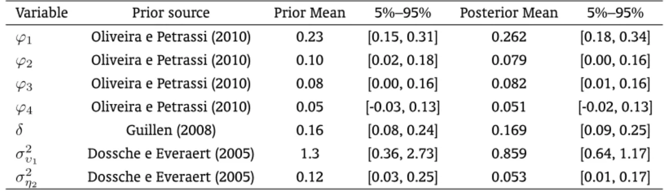
For both the univariate and multivariate estimations, we show two sets of results. First, in Tables 1 and 2, the prior means and distributions of the unobserved coefficients and then their respective posteriors are shown. Second, in Figures 1 and 2 we illustrate key state variables relating to the estimated and perceived targets in comparison to the Brazilian inflation rate.
The univariate case was first estimated, with the decomposition of inflation persistence into intrinsic persistence, derived from the sum of AR coefficients, and into expectations-based persistence, represented by1−δ.
The posteriors obtained for the unobserved components were relatively similar to the values from Brazilian studies used as priors. However, the variancesσυ21andσ
2
η2 proved to be quite different from
Dossche e Everaert (2005) figures. This is due to the different nature of shocks hitting inflation in Brazil and in the euro area.
Table 1: Prior and posterior distributions – Univariate model
Variable Prior source Prior Mean 5%–95% Posterior Mean 5%–95%
ϕ1 Oliveira e Petrassi (2010) 0.23 [0.15, 0.31] 0.262 [0.18, 0.34]
ϕ2 Oliveira e Petrassi (2010) 0.10 [0.02, 0.18] 0.079 [0.00, 0.16]
ϕ3 Oliveira e Petrassi (2010) 0.08 [0.00, 0.16] 0.082 [0.01, 0.16]
ϕ4 Oliveira e Petrassi (2010) 0.05 [-0.03, 0.13] 0.051 [-0.02, 0.13]
δ Guillen (2008) 0.16 [0.08, 0.24] 0.169 [0.09, 0.25]
συ21 Dossche e Everaert (2005) 1.3 [0.36, 2.73] 0.859 [0.64, 1.17]
ση22 Dossche e Everaert (2005) 0.12 [0.03, 0.25] 0.053 [0.01, 0.17]
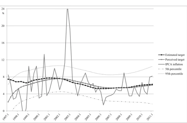
Figure 1 shows the behaviour of state variables in the univariate case compared to IPCA observed inflation. In the first observations, the values are erratic, as a consequence of the filter algorithm. After that, the estimated inflation target had its highest rates around 2001, and then dropped vigorously until the 1st quarter of 2006. After that it has rather stabilized. As for the target perceived by agents, there was a mean-reverting behaviour and, in more recent years, a greater stability and adherence to
8The value ofδ = 0.16means that, on average, 84% of the inflation target perceived by agents, results from the target
the target we estimated to be the actual target followed by the Central Bank. It should be noted that a relatively large uncertainty is present, as the 5th and 95th percentiles show.
Figure 1: Unobserved targets and inflation (yearly, %) – Univariate model
%
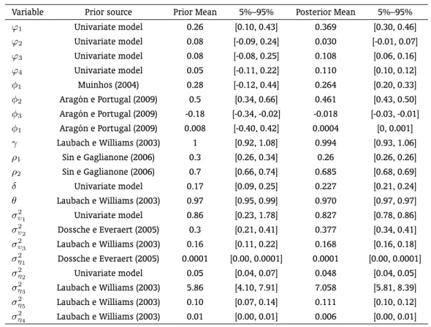
In regard to the results of the multivariate estimation (see Table 2), we have a broader scenario that now includes extrinsic persistence, as mentioned before. The priors generally proved to result in good approximations for most coefficients. The initial profile of the autoregressive coefficients slightly changed, since the 2nd inflation lag(ϕ2)is oddly lower than the 3rd and 4th lags(ϕ3,ϕ4). Dossche e Everaert (2005) found a lower 3rd lag among the results of the euro area. Both their result and ours reflect the importance of the choice of several lags as a measure of intrinsic persistence, as opposed to simply choosing the first lag. More importantly, the sum of autoregressive components resulted in greater intrinsic persistence (0.62 instead of 0.47). On the other hand, lower expectations-based persistence was found (0.77 instead of 0.83). Extrinsic persistence, which is specific to the multivariate setting, summed 0.44.
Together these figures suggest that, on the one hand, extrinsic persistence matters, since its introduction impacts the results of other sources of persistence, but on the other hand, it has a lower share on aggregate persistence than the other two drivers.
Table 2: Prior and posterior distributions – Multivariate model
Variable Prior source Prior Mean 5%–95% Posterior Mean 5%–95%
ϕ1 Univariate model 0.26 [0.10, 0.43] 0.369 [0.30, 0.46]
ϕ2 Univariate model 0.08 [-0.09, 0.24] 0.030 [-0.01, 0.07]
ϕ3 Univariate model 0.08 [-0.08, 0.25] 0.108 [0.06, 0.16]
ϕ4 Univariate model 0.05 [-0.11, 0.22] 0.110 [0.10, 0.12]
φ1 Muinhos (2004) 0.28 [-0.12, 0.44] 0.264 [0.20, 0.33]
φ2 Aragón e Portugal (2009) 0.5 [0.34, 0.66] 0.461 [0.43, 0.50]
φ3 Aragón e Portugal (2009) -0.18 [-0.34, -0.02] -0.018 [-0.03, -0.01]
φ1 Aragón e Portugal (2009) 0.008 [-0.40, 0.42] 0.0004 [0, 0.001]
γ Laubach e Williams (2003) 1 [0.92, 1.08] 0.994 [0.93, 1.06]
ρ1 Sin e Gaglianone (2006) 0.3 [0.26, 0.34] 0.26 [0.26, 0.26]
ρ2 Sin e Gaglianone (2006) 0.7 [0.66, 0.74] 0.685 [0.68, 0.69]
δ Univariate model 0.17 [0.09, 0.25] 0.227 [0.21, 0.24]
θ Laubach e Williams (2003) 0.97 [0.95, 0.99] 0.970 [0.97, 0.97]
σ2
υ1 Univariate model 0.86 [0.23, 1.78] 0.827 [0.78, 0.86]
σ2υ2 Dossche e Everaert (2005) 0.3 [0.21, 0.41] 0.377 [0.34, 0.41]
σ2
υ3 Laubach e Williams (2003) 0.16 [0.11, 0.22] 0.168 [0.16, 0.18]
σ2
η1 Dossche e Everaert (2005) 0.0001 [0.00, 0.0001] 0.0001 [0.00, 0.0001]
σ2
η2 Univariate model 0.05 [0.04, 0.07] 0.048 [0.04, 0.05]
σ2
η3 Laubach e Williams (2003) 5.86 [4.10, 7.91] 7.058 [5.81, 8.39]
σ2
η5 Laubach e Williams (2003) 0.10 [0.07, 0.14] 0.111 [0.10, 0.12]
σ2
η4 Laubach e Williams (2003) 0.01 [0.00, 0.01] 0.006 [0.00, 0.01]
two sources. Therefore, this result actually means that persistence of expectations plays a major role on aggregate persistence.
Consolidated estimates of the relevant parameters for the sources of persistence are shown in the first columns of Table 3. Departing from the univariate to the multivariate approach, there is a decrease in expectations-based persistence and an increase in intrinsic persistence. The reduction in expectations-based persistence is probably an effect of the introduction of extrinsic persistence, as already mentioned. The resultδ= 0.23demonstrates that the speed of expectations updating is higher than what would be expected from “sticky information” estimates produced by Guillen (2008) for Brazil. Still it shows that expectation persistence is higher than intrinsic inflation persistence, measured by P
ϕi, for both models. This result is in line with Dossche e Everaert (2005) findings for the US and the
Euro Area.
We also estimate the same model, considering two alternative periods. The periods were formed removing 16 quarters from each extremity. Thus, the first period starts in 1995 and ends in 2007, while the second term consists of 1999-2011. In the choice of the number of observations we had in mind the accuracy of estimations; obviously the division into two separate periods would generate inaccurate results, due to the number of unobserved variables. Moreover, the second period coincides with the inflation-targeting era in Brazil.
Figure 2: Unobserved targets and inflation (yearly %) – Multivariate model
%
expectations to its actual targets, as a result of credibility improvements. Nevertheless, as already pointed out, expectation distortions have clearly been a key source of persistence over all periods, as opposed to the traditional view of intrinsic persistence. This finding stays in line with the Euro area and US results from Dossche e Everaert (2005).
Table 3: Summarized measures of persistence
Variable Univariate Multivariate Multivariate 1stperiod Multivariate 2ndperiod
(1995-2011) (1995-2011) (1995-2007) (1999-2011) P
ϕi 0.47 0.62 0.60 0.38
(1−δ) 0.83 0.77 0.81 0.78
ϕ2+φ3 – 0.44 0.33 0.35
Extrinsic persistence, on the other hand, has not quite changed over the periods considered and was considerably lower than the one found in the Euro area and in the US. Therefore, persistent deviations of output from its natural level may be more present in these developed economies than in Brazil.
Oliveira e Petrassi (2010) in a similar period.9 Dossche e Everaert (2005) also reported similar findings
when comparing their intrinsic persistence results with the ones from univariate frameworks in the USA and in the euro zone. However they do not consider alternative periods.
Finally, we provide estimates of the natural rate of interest. In our model, its introduction prevented shifts in the actual inflation target from being affected by changes in the benchmark that represents the natural rate of interest. Equations (11) through (13) determine the evolution of the equilibrium interest rate over time, together with the trend growth rate and the parameter that measures time preferences. The declining trend seen in Figure 3, even considering wide confidence bands, is in line with recent estimations from the Central Bank of Brazil (see BCB, 2010, 2012).10 As for its determinants,
shifts in the trend growth rate did not seem to significantly affect the recent behaviour of the natural rate of interest, as did shifts in time preferences. The same pattern was observed in the data obtained by Dossche e Everaert (2005) for the Euro zone and the USA.
Figure 3: Natural vs. actual real interest rates (yearly, %)
%
We also compared the estimated natural rates of interest with actual real interest rates, computed by simply subtracting the observed IPCA inflation from nominal interest rates for each quarter, that is,rt=πt−it. If the monetary authority follows a neutral stance regarding policy rate adjustment,
both rates should ideally evolve similarly. Considering the whole period, this is certainly not the case, but if we take into account only the period under the inflation targeting regime, interest rate gaps are relatively smaller considering historical interest rate figures. Of course, one has to bear in mind that these are ex-post figures.
9Their intrinsic persistence estimates for the 1995 to 2009 period range from 0.416 to 0.509, whereas our main result for the
univariate model was 0.47.
10The Central Bank of Brazil reports the drivers for this decline in the natural rate of interest. For a review on alternative
5. CONCLUSIONS
The aim of this paper was to measure inflation persistence for a recent time period in Brazil, and also to identify the types of inflation persistence using three major sources: intrinsic, extrinsic, and expectations-based.
Aside from the usual intrinsic persistence, the impact of macroeconomic shocks, such as output deviations, on persistence, which lead to extrinsic persistence, was also determined. It was also assumed that shifts in the inflation target (which are not always known and perceived by all agents) may result in permanent changes in mean inflation. Private agents’ perception of the policy target sometimes differs considerably from the actual target followed by the central bank, which also induces inflation persistence. These facts are often not considered by conventional empirical models when measuring persistence.
Following Dossche e Everaert (2005), the inflation generating process was decomposed11 into unobserved variables using the Kalman filter. The main contributions were the following: first, this type of estimation is novel for Brazil, because the dynamics of inflation and of its determinants are jointly assessed in a model that contemplates not only the sticky price behaviour, but also the idea of sticky information. Second, by clarifying inflation persistence in Brazil and simultaneously adding more information on the natural rate of interest, this study provides important data that may enrich the framework of monetary policy in the country.
The following major results were obtained. First, the role of inflation expectations, of shifts in inflation targets, and of significant deviations of output and of the natural rate of interests in inflation persistence should not be neglected in any representation of inflation dynamics. Not surprisingly, the impact of accounting for such factors in measures of inflation persistence is that the usual intrinsic persistence is quite different from traditional figures from univariate approaches. These factors are especially important for Brazil, which has gone through the implementation of an inflation targeting regime and episodes of inflation during foreign crises and the domestic crisis in 2002/2003. Second, although intrinsic inflation persistence has significantly decreased in the past few years, the other two sources did not experience such a trend. Hence, one should cautiously interpret literature findings that point to an undisputable decrease in inflation persistence, especially if they are based on intrinsic measures of persistence. As we particularly showed, expectations-based persistence proved to be both high and almost unchanged over recent years. Similarly to Portugal e Neto (2009) and estimates from recent Inflation Reports, we conclude that natural interest rates have been declining. Of course one should be cautious since we deal with a restricted period and the natural rate of interest entails a long-run definition.
BIBLIOGRAFIA
Angeloni, I., Aucremanne, L., Ehrmann, M., Gali, J., Levin, A., & Smets, F. (2004). Inflation persistence in the Euro area: Preliminary summary of findings. InECB Conference on Inflation Persistence in the Euro Area.
Aragón, E. & Portugal, M. (2009). Central bank preferences and monetary rules under the inflation targeting regime in Brazil. Brazilian Review of Econometrics, 29:79–109.
Baillie, R. T., Chung, C.-F., & Tieslau, M. (1996). Analysing inflation by the fractionally integrated ARFIMA-GARCH model.Journal of Applied Econometrics, 11:23–40.
BCB (2003). Open letter to the finance minister. Banco Central do Brasil.
11In the present study, we only consider the IPCA (broad consumer price index). However, a possible extension could deal with
BCB (2008). Inflation report. Banco Central do Brasil, 151–155.
BCB (2010). Inflation report. Banco Central do Brasil, 94–103.
BCB (2012). Inflation report. Banco Central do Brasil, 89–97.
Bogdanski, J., tombini, A., & Werlang, S. (1999). Implementing inflation targeting in Brazil. Working Paper 1, Banco Central do Brasil.
Caetano, S. & Moura, G. (2009). Reajuste informacional no Brasil: Uma aplicação da curva de Phillips sob rigidez de informação. InAnais do XXXVII Encontro Nacional de Economia.
Calvo, G. A. (1983). Staggered prices in a utility-maximizing framework. Journal of Monetary Economics, 12:383–398.
Campelo, A. K. & Cribari-Neto, F. (2003). Inflation inertia and inliers: The case of Brazil.Revista Brasileira de Economia, 57:713–739.
Cecchetti, S. G. & Debelle, G. (2006). Has the inflation process changed? Economic Policy, 21:311–352.
Cogley, T. & Sargent, T. J. (2005). Drifts and volatilities: Monetary policies and outcomes in the post WWII US. Review of Economic Dynamics, 8:262–302.
Cukierman, A. & Meltzer, A. H. (1986). A theory of ambiguity, credibility, and inflation under discretion and asymmetric information. Econometrica, 54:1099–1128.
Dossche, M. & Everaert, G. (2005). Measuring inflation persistence: A structural time series approach. Working Paper 495, ECB.
Durevall, D. (1999). Inertial inflation, indexation and price stickiness: Evidence from Brazil. Journal of Development Economics, 60:407–421.
Figueiredo, E. A. & Marques, A. M. (2011). Inflação inercial sob mudanças de regime: Análise a partir de um modelo MS-ARFIMA. Economia Aplicada, 15:443–457.
Giammarioli, T. & Valla, N. (2004). The natural real interest rate and monetary policy: A review. Journal of Policy Modeling, 26:641–660.
Gomes, C. & Leme, M. C. S. (2011). An analysis of the degree of persistence of inflation, inflation expectations and real interest rate in Brazil.Revista Brasileira de Economia, 65:289–302.
Gomes, C., Lopes, D. T., & Rebelo, A. M. (2011). Persistência inflacionária: Comparações entre três economias emergentes.Revista de Economia e Administração, 10:152–167.
Gomes, C. & Vieira, F. V. (2013). Persistência inflacionária regional brasileira: Uma aplicação dos modelos ARFIMA. Economia Aplicada, 17:117–136.
Guillen, D. (2008). Ensaios sobre a formação de expectativas de inflação. Dissertação de mestrado, Faculdade de Economia, PUC-Rio.
Koopman, S. & Durbin, J. (2003). Filtering and smoothing of state-vector for diffuse state-space models.
Journal of Time Series Analysis, 24:85–98.
Laubach, T. & Williams, J. C. (2003). Measuring the natural rate of interest. The Review of Economics and Statistics, 85:218–231.
Levin, A. T. & Piger, J. M. (2004). Is inflation persistence intrinsic in industrial economies? Working Paper 334, ECB.
Mankiw, N. G. & Reis, R. (2002). Sticky information versus sticky prices: A proposal to replace the new Keynesian Phillips curve.The Quarterly Journal of Economics, 117:1295–1328.
Mankiw, N. G., Reis, R., & Wolfers, J. (2003). Disagreement about inflation expectations. In NBER Macroeconomics Annual, volume 18, pages 209–270. NBER.
Marques, C. R. (2004). Inflation persistence: Facts or artefacts? Working Paper 371, ECB.
Milani, F. (2007). Expectations, learning and macroeconomic persistence.Journal of Monetary Economics, 54:2065–2082.
Oliveira, F. N. & Petrassi, M. (2010). Is inflation persistence over? BCB Working Paper 230, Banco Central do Brasil.
Pincheira, P. (2009). La dinámica de la persistencia inflacionaria en Chile. Investigación de Banco Central de Chile 12, Banco Central de Chile.
Pivetta, F. & Reis, R. (2007). The persistence of inflation in the United States. Journal of Economic Dynamics and Control, 31:1326–1358.
Portugal, M. & Neto, P. C. (2009). The natural rate of interest in Brazil between 1999 and 2005. Revista Brasileira de Economia, 63:103–118.
Rudebusch, G. & Svensson, L. (1999). Policy rules for inflation targeting. InMonetary Policy Rules, pages 203–262. University of Chicago Press.
Sims, C. A. (2003). Implications of rational inattention.Journal of Monetary Economics, 50:665–690.
A. APPENDIX: STATE-SPACE REPRESENTATIONS AND BAYESIAN INFERENCE
A usual linear Gaussian state space model is given by
yt = Zat+Adt+εt
at = T at−1+Rηt
whereZandAare coefficient matrices,dtis a vector of exogenous variablesK×1, andεtis an error
vector, such that E(εt) = 0 andV ar(εt) = H. Also, T and Rare coefficient matrices, andηtis
an error vector with zero mean andV ar(ηt) = Q. As in Dossche e Everaert (2005), the filtering and
smoothing algorithms were modified to account for diffuse initialization ofa1. This procedure is well described in Koopman e Durbin (2003).
In state space form we may express the univariate model (equations 3 through 6) using the above notation as following:
yt = [πt] H =
σ2υ1
Z = " 1− 4 X i=1 ϕi ! 0 # T = "
2−δ δ−1
1 0
#
at = πtPπtP−1 ′ R= " δ 0 #
A = [ϕ1ϕ2ϕ3ϕ4] ηt= [η2t]
dt = [πt−1πt−2πt−3πt−4]′ Q=σ2η2
εt = [υ1t]
Analogously, the equations of the multivariate model can be represented in state space form, as follows:
yt = [πtityτt]′
Z =
0 (1−P
ϕi) 0 0 −φ1 0 0 0 0 0
ρ1 (1−ρ2) 0 0 0 0 (1−ρ2)γ 0 (1−ρ2) 0
0 0 φ4 1 −φ2 −φ3 0 φ4γ 0 φ4
αt =
πT
tπtPπtP−1ytPytP−1yPt−2λtλt−1τtτt−1 ′
A =
ϕ1 ϕ2 ϕ3 ϕ4 φ1 0 0
ρ1 0 0 0 0 0 ρ2
0 0 0 0 φ2 φ3 −φ4
dt = [πt−1πt−2πt−3πt−4yt−1yt−2it−1]′
εt = [υ1tυ2tυ3t]′
H =
συ21 0 0
0 σ2−υ
2 0
0 0 σ2υ3
T =
1 0 0 0 0 0 0 0 0 0
δ (1−δ) 0 0 0 0 0 0 0 0
0 1 0 0 0 0 0 0 0 0
0 0 0 1 0 0 1 0 0 0
0 0 0 1 0 0 0 0 0 0
0 0 0 0 1 0 0 0 0 0
0 0 0 0 0 0 1 0 0 0
0 0 0 0 0 0 1 0 0 0
0 0 0 0 0 0 0 0 θ 0
0 0 0 0 0 0 0 0 1 0
R =
0 1 0 0 0
1 δ 0 0 0
0 0 0 0 0 0 0 1 1 0 0 0 0 0 0 0 0 0 0 0 0 0 0 1 0 0 0 0 0 0 0 0 0 0 1 0 0 0 0 0
ηt = [η1tη2tη3tη4tη5t]′
Q =
η1t 0 0 0 0
0 η2t 0 0 0
0 0 η3t 0 0
0 0 0 η4t 0
0 0 0 0 η5t
Operationalization of the usual algorithm of the Kalman filter requires that matricesZ, A, H, T, R
and Q be known. Since they depend on a vector of unknown parameters ψ, it is necessary to additionally make an inference about this vector. Including data obtained from other studies, it is possible to treat ψas a vector of random parameters with prior density p(ψ)and to estimate the posterior densityp(ψ|y)using Bayesian inference. Alternatively, the goal is to find the posterior mean
¯
ggiven by:
¯
g=E[g(ψ|y)] =
Z
g(ψ)p(ψ|y)dψ
Following Dossche e Everaert (2005) and using Bayes’ theorem, this turns into:
¯
g=
R
g(ψ)zg(ψ,y)g(ψ|y)dψ
R
zg(ψ,y)g(ψ|y)dψ
where
zg(ψ,y) =p(ψ)p(y|ψ)
Departing from a sample ofnindependent choices ofψ, calledψ(i), we obtain ag¯
nestimator ofg¯:
¯
gn=
Pn
i=1g(ψ(i))zg(ψ(i),y) Pn
i=1zg(ψ(i),y)
In practice, we introduce estimators of the posterior mean ofψ¯ = E(ψ|y). This is possible by admittingg(ψ(i)) =ψ(i)andψ˜= ¯g
nin the previous equation, whereψ˜is the estimator ofψ¯. The 5th
and 95thpercentiles are also computed. Briefly, an estimate of the 5thpercentile,ψ˜5%, derives from
F( ˜ψ5%|y) = 0.05, whereF( ˜ψ|y) =P rob(ψ(i)
j ≤ψj)denotes thejthelement inψ. The same applies