Fiscal Policy Responiveness, Persistence and Discretion

Carlos Pestana Barros & Nicolas Peypoch

A Comparative Analysis of Productivity Change in Italian and Portuguese Airports

WP 006/2007/DE _________________________________________________________

António Afonso, Luca Agnello and Davide Furceri

Fiscal Policy Responiveness, Persistence and Discretion

WP 50/2008/DE/UECE _________________________________________________________

Department of Economics

WORKING PAPERS

ISSN Nº0874-4548

School of Economics and Management

Fiscal Policy Responsiveness, Persistence,

and Discretion

*

António Afonso,

Luca Agnello,

Davide Furceri

October 2008

Abstract

We decompose fiscal policy in three components: i) responsiveness, ii) persistence and iii) discretion. Using a sample of 132 countries, our results point out that fiscal policy tends to be more persistent than to respond to output conditions. We also found that while the effect of cross-country covariates is positive (negative) for discretion, it is negative (positive) for persistence thereby suggesting that countries with higher persistence have lower discretion and vice versa. In particular, while government size, country size and income have negative effects on the discretion component of fiscal policy, they tend to increase fiscal policy persistence.

JEL: E62, H50.

Keywords: Fiscal Policy, Fiscal Volatility.

* _{We are grateful to Jacopo Cimadomo, Javier Pérez, Ad Van Riet, Jürgen von Hagen, participants at an ECB}

seminar, and to Silvia Albrizio and Matthijs Lof for research assistance. The opinions expressed herein are those of the authors and do not necessarily reflect those of the ECB or the Eurosystem.

#

European Central Bank, Directorate General Economics, Kaiserstraße 29, D-60311 Frankfurt am Main, Germany, email: antonio.afonso@ecb.europa.eu.

$

ISEG/TULisbon – Technical University of Lisbon, Department of Economics; UECE – Research Unit on Complexity and Economics, R. Miguel Lupi 20, 1249-078 Lisbon, Portugal, email: aafonso@iseg.utl.pt. UECE is supported by FCT (Fundação para a Ciência e a Tecnologia, Portugal), financed by ERDF and Portuguese funds.

♦ _{University of Palermo, Department of Economics, Italy, emails: furceri@.economia.unipa.it}

luca.agnello@economia.unipa.it. Luca Agnello would like to thank the Fiscal Policies Division of the ECB for its hospitality.

♠

Contents

Non-technical summary ... 3

1. Introduction... 5

2. Literature... 7

3. Empirical Strategy ... 11

3.1 Fiscal Measures of Responsiveness, Persistence and Discretion... 11

3.2 What Matters for the Fiscal Measures? ... 12

4. Results and discussion ... 14

4.1 Quantitative Estimates for Responsiveness, Persistence and Discretion... 14

4.2 Determinants of the Fiscal Measures... 16

4.3 Robustness Analysis ... 21

5. Conclusion ... 23

References... 23

Appendix 1 – Data and sources ... 37

Non-technical summary

In the last decade, several studies in the economic literature have assessed fiscal policy

characteristics. Most of these studies analyze the responsiveness of fiscal policy, that is,

the response of fiscal policy to output. Other contributions analyze the extent to which

fiscal discretion impacts on the macroeconomic environment with the final objective to

solve the trade-off between the degree of fiscal discipline and the necessary flexibility to

deal with automatic stabilizers. Interestingly, few empirical studies asses the relevance of a

third fiscal policy characteristic: persistence. Generally speaking, fiscal persistence can be

considered as a measure of the degree of dependence of current fiscal behaviour on its own

past developments. We contribute to the literature by providing evidence that also accounts

for this latter fiscal characteristic.

In particular, we extend the analysis of Fatás and Mihov (2003, 2006) in several ways: i)

we also compute a measure of fiscal persistence, allowing to cross-check persistence and

discretion; ii) the abovementioned three fiscal components are obtained both for

government spending and revenue; iii) we analyse the determinants of all three fiscal

components with a set of macroeconomic, political and institutional variables, and

geographical variables; iv) finally we also use several datasets.

In order to pursue our objectives we employ a two-stage empirical strategy. In the fist

stage, we decompose fiscal policy, and in more detail government spending and revenues,

in three components: i) responsiveness, ii) persistence and iii) discretion. In the second

stage of our analysis, using the estimates of responsiveness, persistence and discretion, we

employ a cross-country analysis in order to identify the common set of economic, political

Our analysis covers a set of 132 developed and developing countries over the period

1980-2007, as well as data for EU-15 countries over the period 1970-2007. The main results of

the paper can be summarized as follows: a) fiscal policy is not responsive in most of the

countries in the sample (i.e. responsiveness is generally small and in many cases not

statistically significant) while persistence is the dominant component; b) more

interestingly, there exists a significant trade-off between persistence and discretion. Both

for revenue and spending, persistence is negatively correlated to the discretion component

thereby suggesting that countries with higher persistence have lower discretion. These

findings are supported by the results of the second part of the analysis where we carry out

a cross-country estimation approach to identify the source of fluctuations of both

persistence and discretion components. According to the previous empirical finding,

suggesting that a negative relationship between discretion and persistence exists, we find

that while government size, country size and income have negative effects on the

discretion component of fiscal policy, they tend to increase fiscal policy persistence.

Moreover, we find that macro and political and institutional variables are less relevant for

1. Introduction

In the last decade, several studies in the economic literature have assessed fiscal

policy characteristics. Most of these studies analyze the responsiveness of fiscal policy,

that is, the response of fiscal policy to output, in order to explore the effectiveness of

automatic stabilizers. Other contributions analyze the extent to which fiscal discretion

impacts on the macroeconomic environment.

Interestingly, few empirical studies asses the relevance of a third fiscal policy

characteristic: persistence. Generally speaking, fiscal persistence can be considered as a

measure of the degree of dependence of current fiscal behaviour on its own past

developments. We contribute to the literature by providing evidence that also accounts for

this latter fiscal characteristic. In particular, the aim of this paper is to disentangle fiscal

policy (both government spending and revenue) in three components: responsiveness,

persistence and discretion, and to assess which variables make these components to vary

across countries. Thus, compared to existing work on the literature, we provide a broader

and more comprehensive approach to assess the behaviour of fiscal policy (in terms of

responsiveness, persistence and discretion) and its determinants.

In particular, we extend the analysis of Fatás and Mihov (2003, 2006) in several

ways: i) we also compute a measure of fiscal persistence, allowing to cross-check

persistence and discretion; ii) the abovementioned three fiscal components are obtained

both for government spending and revenue; iii) we analyse the determinants of all three

fiscal components with a set of macroeconomic, political and institutional variables, and

geographical variables; iv) finally we also use several datasets.

From a methodological point of view, we consider the elasticity of government

revenues and expenditures to output as a measure of the fiscal responsiveness to economic

processes describing the behaviour of both government expenditures and revenues.

Finally, we identify discretion as the part of government spending and revenue that does

not correspond to systematic responses to output conditions and in past values of

government spending and revenue, but is instead the consequence of exogenous political

processes or extraordinary non-economic circumstances.

Our analysis covers a set of 132 developed and developing countries over the

period 1980-2007, as well as data for EU-15 countries over the period 1970-2007. The

main results of the paper can be summarized as follows: a) fiscal policy is a-cyclical in

most of the countries in the sample (i.e. responsiveness is generally small and in most of

the cases not statistically significant) while persistence is the dominant component; b)

more interestingly, there exists a significant trade-off between persistence and discretion.

Both for revenue and spending, persistence is negatively correlated to the discretion

component thereby suggesting that countries with higher persistence have lower discretion.

These findings are supported by the results of the second part of the analysis. In fact, we

found that regressing both discretion and persistence estimates on a common set of

explanatory variables, the sign of the coefficient associated to many of these cross-country

covariates is opposite in the two regressions.

Moreover, we find that macro and political and institutional variables can not

account for responsiveness, once regional dummies are considered.

The rest of the paper is organized as follows. Section two briefly reviews the

related literature. Section three explains the empirical strategy used to identify the

responsiveness, persistence and discretionary parts of both government spending and

revenue. It also illustrates the strategy used to identify the determinants of fiscal

presents and discusses the results. Section five concludes with the main findings, policy

implications and suggestion for future works.

2. Literature

The existing related literature has usually analyzed two of three abovementioned

components of fiscal policy. On the one hand, the responsiveness of fiscal policy to output,

and on the other hand, the discretionary part of fiscal policy. These two issues have

deserved great interest since both are crucial for output stabilization and, therefore,

indirectly for growth and aggregate welfare1.

The issue of responsiveness of fiscal policy has received increasing attention from

researchers both from a theoretical and empirical point of view.

From a theoretical point of view, standard Keynesian models imply that fiscal

policy should be counter-cyclical, i.e. government spending (taxes) should rise (decrease)

in recessions and increase in booms. At the other stream, tax-smoothing models inspired

by Barro (1979) imply that government will smooth both tax rate and government

spending by borrowing in recessions and repaying in booms, i.e. government spending will

be uncorrelated with changes in GDP, while tax revenue will be positively correlated.

From an empirical point of view, the evidence is quite mixed, varying across

spending and revenues categories as well as across countries. For OECD countries, some

research shows that spending is counter-cyclical (Gali, 1994), while others show no

discernible pattern (e.g. Fiorito, 1997; Gavin and Perotti, 1997b). The differences in these

results depend on the components of spending being measured. For example, Gali (1994)

studies government consumption and investment in a simple cross-country regression for a

sample of 22 OECD countries and finds that both taxes and government purchases seem to

1

be effectively working as "automatic stabilizers", with government purchases following a

counter-cyclical pattern. Fiorito and Kollintzas (1994) and Fiorito (1997), on the other

hand, study specifically government consumption in the G-7 countries and find that the

expenditures are either counter-cyclical or a-cyclical.

The limited number of empirical studies for developing countries suggests that

government spending tends to be pro-cyclical. For example, Gavin and Perotti (1997a)

find that fiscal policy is highly pro-cyclical in Latin America; Kaminsky, Reinhart, and

Vegh (2004) find that fiscal policy is pro-cyclical in their sub-sample of 83 low- and

middle-income countries; Braun (2001) finds that government expenditure is pro-cyclical

in a panel of 35 developing countries for the period 1970-1998.

The conventional wisdom that emerges from these studies is that fiscal policy is

counter-cyclical or a-cyclical in most developed countries, while it is pro-cyclical in

developing countries. This result is corroborated by Lane (2003) who finds that the

capability to implement fiscal control procedures is positively correlated with the level of

development (measured by output per capita). This implies that richer countries enjoy less

pro-cyclical government spending.

Several explanations have been advanced to explain the cross-country variation in

the degree of fiscal cyclicality especially between developing and industrial countries.

Important factors behind cyclicality of fiscal policy are political and institutional

ones. For example, Talvi and Vegh (2005) find that pro-cyclicality of fiscal policy is

related to political distortions. They develop an optimal fiscal policy model in which

running budget surpluses is costly because they create pressures to increase public

spending. Given this distortion, a government that faces large fluctuations in the tax base

will find it optimal to run pro-cyclical fiscal policy. Considering the differences in tax base

appears to be broadly consistent with Barro’s tax smoothing proposition, in developing

countries government spending and taxes are highly pro-cyclical.

Persson (2001), Persson and Tabellini (2001), Alesina and Tabellini (2005), also

find that political and institutional factors matter also for fiscal responsiveness. In

particular, while Persson (2001) and Persson and Tabellini (2001) find that parliamentary

and majority based systems are related to cyclicality of fiscal policy, Alesina and Tabellini

(2005) show that most of the pro-cyclicality of fiscal policy in developing countries can be

explained by high levels of corruption.

Hallerberg and Strauch (2002) argue that fiscal policy is less anti-cyclical in the

Economic and Monetary Union (EMU) countries in election years. Similar results in U.S.

states are documented by Sorensen, Wu and Yosha (2001). Using data for OECD

countries, Lane (2003) shows that countries with volatile output and dispersed political

power are the most likely to run pro-cyclical fiscal policies.

Finally, an interesting contribution is the work of Galì and Perotti (2003). After

estimating fiscal policy rules for eleven EMU countries over the period 1980-2002, they

test whether fiscal constraints of the EMU – as embedded in the Maastricht Treaty and the

Stability Growth Path – may be conducive of pro-cyclical fiscal policies. According to

their results, anti-cyclical policies became stronger after the adoption of the Maastricht

Treaty. Galì (2005) demonstrates that this latter evidence holds in general for all

industrialized countries. Afonso (2008) also finds evidence of counter-cyclical responses

of fiscal policy for the EU countries.

The second issue of fiscal policy that has been considered in the literature regards

the discretionary component of fiscal policy. A large number of studies provide evidence

that discretionary spending is strongly and negatively related to the quality of institutions

political and institutional determinants of discretionary fiscal policy and their effects on

output volatility and economic growth. They use the term discretionary to refer to changes

in fiscal positions that represent neither automatic reaction to economic conditions nor can

be related to persistent changes in budget items. Using data from 91 countries, they find

that highly volatile discretionary fiscal policy exerts a strong destabilizing effect on the

economy. Additionally, fiscal policy is explained to a large extent by such variables as the

characteristics of electoral and political systems and the lack of political constraints. They

conclude that institutional arrangements that constrain discretion via checks and balances

allow nations to achieve higher rates of economic growth and reduce macroeconomic

instability.

More recently, Fatás and Mihov (2006), using data from 48 US states, explore the

role that “rules” and institutions play in determining discretionary fiscal policy and look at

whether the same rules and institutions influence the cyclicality of fiscal policy.

Cyclicality is defined as the elasticity of government spending with respect to output. They

find that strict budgetary restrictions lead to lower policy volatility and reduce the

responsiveness of fiscal policy to output shocks. These two results should have opposite

effects on output volatility. While less discretion should reduce volatility, less

responsiveness of fiscal policy might amplify business cycles.

According to the empirical evidence reviewed above, political and institutional

variables can affect the composition of government spending in its discretionary,

persistence and responsiveness components. Thus, ultimately, it is natural to expect that

countries differ in the behaviour of both government spending and revenue along these

3. Empirical Strategy

3.1 Fiscal Measures of Responsiveness, Persistence and Discretion

Following Fatás and Mihov (2003, 2006), in order to differentiate between

persistence, responsiveness and discretion in government spending and revenue we

estimate for each country i (with i =1,…,N ) the following regressions:

( )

( )

(

)

t i t i G i t i G i t i G i G i t

i Y G

G_, log _, log _{, 1 , ,}

log =α +β +γ ₋ +δ Z +ε (1)

log

( )

( )

(

)

where G is real government spending, R is real government revenue, Y is real GDP, and Z

is a set of controls including also time trend2.

The estimates of the country-specific coefficients βi, γi and σi in (1) and in (2)

(where σi is the standard deviation of the residuals of the above regressions) will represent

respectively our measures of responsiveness, persistence, and a quantitative estimate of

discretionary fiscal policy. In order to get these estimates, we include as control variables

(i.e. the vector Zi) the current and the lagged value of real oil prices, the current inflation

rate and a linear time trend. Oil prices are included since they affect the state of the

economy and more importantly because they contribute significantly to total revenue for

some of the countries in the sample. We include inflation to ensure that our results are not

driven by high inflation episodes. We also consider a time trend in our specifications, since

government spending and revenue can also have a deterministic time trend in addition to

the stochastic one. Finally, in order to control for possible endogeneity we use past values

of real GDP as instruments.

2

3.2 What Matters for the Fiscal Measures?

Once we obtain the estimates for responsiveness ( GR i

,

ˆ

β ), persistence ( GR i

,

ˆ

γ ) and

discretion ( GR i

,

ˆ

σ ) of fiscal policy we can explain cross-country variation in fiscal policy

behaviour, regressing those estimates on a set of explanatory variables that the literature

has found to be related to fiscal policy.

We estimate the following three cross-country equations (six considering both

estimations for the spending and the revenue equation):

( )

_∑

_∑

_∑

j j ij j j ij j j ij i R

G

i α δ D φ P θ E ξ

σ_ˆ , ₁

log (3)

∑

∑

∑

+ =

j j ij j j ij j j ij i R

G

i α δ D φ P θ E υ

γ_ˆ , _{2 (4)}

∑

∑

∑

+ =

j j ij j j ij j j ij i R

G

i α δ D φ P θ E ω

βˆ , _{3 (5)}

for i = 1,…, N and where: Ej denotes macroeconomic variables; Pj denotes political and

institutional variables; Dj denotes demographic and geographical variables; ω,ν, and ξ are

well-behaved residuals; α’s are nuisance coefficients; δ, φ, and θ are our coefficients of

interest.

In more detail, the set of controls consists of the following variables:3

i) Macroeconomic variables (E): a) GDP per capita; b) openness; c) GDP

deflator-based inflation rate; d) government size, and e) country size .4

ii) Political and institutional variables (P): a) an index of the level of democracy; b) an

index for political stability; c) an index for presidential versus parliamentary electoral

3

See Appendix 1 for a detailed description of the variables and sources.

4

system, d) an index that accounts for constitutional limits on the number of years the

executive can serve before new elections; e) an index of government effectiveness; f) the

Herfindahl index of parties concentration in the government, g) a dummy if the chief

executive is a military chief.5

iii) Geographical variables (D)6: a) the log of absolute latitude (kilometres from the

equator); b) regional dummies for developing countries from b1) Latin America, b2)

Sub-Saharan Africa, b3) East Asia, b4) South Asia, b5) Europe-Central Asia, b6) and Middle

East-North Africa.7

Since our dependent variables are based on estimates, the regression residuals can

be thought of as having two components. The first component is sampling error (the

difference between the true value of the dependent variable and its estimated value). The

second component is the random shock that would have been obtained even if the

dependent variable was directly observed as opposed to estimated. This would lead to an

increase in the standard deviation of the estimates, which would lower the t-statistics. This

means that any correction to the presence of this un-measurable error term will increase

the significance of our estimates8.

We estimate equations (4)-(5) by Weighted Least Squares (WLS). This choice

takes account of the fact that the dependent variables are measured with different degrees

5

The economic literature has generally focused on political and institutional characteristics to explain cross country differences in government spending (Drazen, 2000; Persson, 2001; Persson and Tabellini, 2001). See Fatás and Mihov (2003) for a more detailed discussion.

6

Alesina and Wacziarg (1998) have found that geographical variables are important to explain cross country differences in government spending.

7

As suggested by La Porta et al. (1999), it is likely that latitude from the equator, income and regional dummies are related to the quality of government and institutions.

8

of precision across countries, and of the fact that some of the estimated values of our

dependent variables are not statistically significant from zero.9

4. Results and discussion

We use data from the IMF World Economic Outlook for a set of 132 countries for

which we have data available from 1980 to 2007 (see the data Appendix for further

details).10 Moreover, using data from the European Commission AMECO database, we

perform a similar exercise for the 15 “old” members of the European Union (EU-15), for

which the time sample broadly spans between 1960 and 2007.

4.1 Quantitative Estimates for Responsiveness, Persistence and Discretion

We start our empirical analysis by estimating the coefficients of responsiveness,

discretion and persistence. The results relative to both government spending and revenue,

for the entire set of countries are reported in Table 1. Looking at the table it is possible to

see that in terms of magnitude the coefficient of persistence in the great majority of the

cases is bigger than the one of responsiveness. This is also confirmed by the fact, that

while the coefficient of persistency is statistically significant in most of the cases (73 times

for spending and 68 times for revenue) the coefficient used as our measure of fiscal

responsiveness is statistically significant for a smaller number of cases (42 times for

spending and 48 for revenue). Thus, it seems that overall, fiscal policy tends to be more

persistent than to respond to current output conditions. Moreover, it is interesting to note

that while government revenue reacts relatively more to output than government spending,

spending overall seems to be more persistent than revenue.

9

See, Lane (2003) for a similar approach. All the results presented do not qualitatively change when we estimate equations (3)-(5) by OLS.

10 _{We have also analyzed data from the World Development Indicator CD-ROM 2007. The results with this}

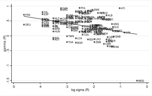
We remark thatour discretion estimates are computed as the standard deviation of

the residuals from both government spending and revenue equations. Thus, it is clear that

the lower and less significant are the coefficients of responsiveness and persistence the

higher will be the component of discretion11. This argument, together with the fact that

fiscal policy seems to be more persistent than responsive, suggests a negative relation

between the measures of persistence and discretion. This intuition is empirically

confirmed. Figure 1 provides the scatter plot of our measures of persistence against

discretion exhibiting a negative relation between these two variables. In particular, the

estimate of this simple bivariate relation for the spending equation is:

( )

with R2 = 0.18 (t statistics are in parenthesis). The negative relationship also holds for the

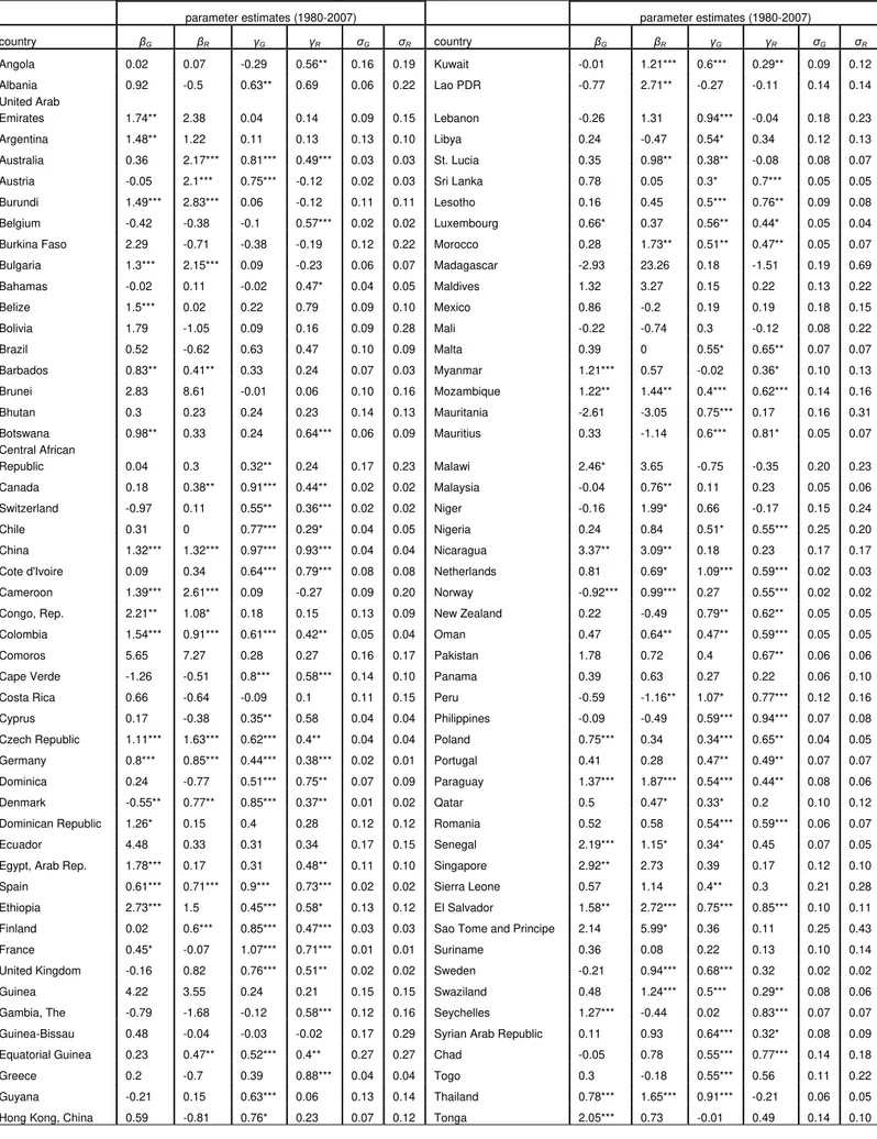
revenue equation (see Figure 2):12

( )

with R2 = 0.12 (t statistics are in parenthesis). Thus, it seems that countries with higher

persistence have a lower discretionary component of fiscal policy. In Table 2 we also

report a rank analysis for our measure of persistence and discretion.

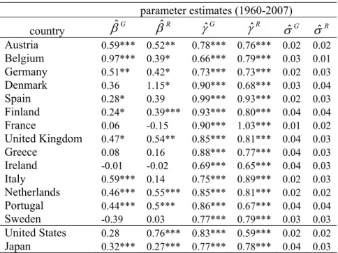
In order to check for the robustness of our results, we consider another data source

for both revenues and government spending: the AMECO dataset comprising data from

1960 to 2007 for European Union countries. Therefore, we have considered the “old”

EU-15 countries, with exception of Luxemburg, for which data are not available for the period

11 In fact, the lower the significance of the coefficients, the lower the R-squared of the regression, and the higher the variance of the residuals.

12 _{The correlation between} G i

γˆ and ln

( )

( )

1988-89. For comparative purposes, we have decided to include also the United States and

Japan.

Table 3 reports parameter estimates of responsiveness, persistence and discretion

from the equations (1)-(2) over the sample period 1960-2007. We note that, while

parameter estimates G i

γˆ and R i

γˆ are always statistically significant (at 1% for all countries),

estimates ofβs are significant only for 62% of the cases (10 countries out of 16 for both

revenues and spending). Moreover, we also find a negative correlation betweenγ

coefficients and their corresponding discretionary components. In particular, we find that

the cross-country correlation betweenγˆ and _iG

( )

σˆ

log equals -0.14 while the cross-country

correlation between R i

γˆ and

( )

σˆ

log is -0.32.

The above results corroborate our previous conclusions: a) persistence is the

dominant component of both government spending and revenue while evidence about their

responsiveness to the economic conditions is less clear; b) there is a negative relationship

between the degree of persistence and discretion.

4.2 Determinants of the Fiscal Measures

In the previous section we found a significant and negative relation between

discretion and persistence. On the one hand, this is partly explained by the fact that fiscal

policy is not responsive for many countries in our sample. On the other hand, these results

can be explained by the fact that if spending is left to discretionary actions and political

decision its development will be less persistent, deviating more from the trend.

However, it has to be kept in mind that we cannot infer any causal relation between

these two components of fiscal policy since they are both simultaneously determined by

macroeconomic, institutional, political and geographical variables. Thus, it is also likely to

specification for our measures of persistence and discretion. In other words we expect that

(at least for some variables) if a cross-country covariate has a negative (positive) impact on

discretion it should have a positive (negative) impact on persistence.

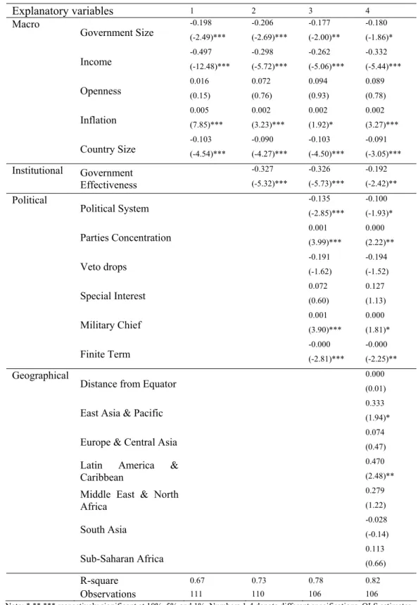
We start our analysis by estimating equation 3 for government spending G in order

to explain the respective discretion component. Results are reported in Table 4. In each

column of the table we present a different specification of the controls. Starting with the

first column, we can see that all the macro variables (with the exception of openness) are

significantly related to discretionary spending and with the expected sign. Discretionary

spending is negatively related to government size, since usually bigger governments have

more stable government spending and automatic stabilizers are larger (Fatás and Mihov,

2001). Income (GDP per capita) is negatively related to discretionary spending, since it is

likely that poorer countries have a more volatile business cycle due to less developed

financial markets, and at the same time may resort more often to discretionary fiscal policy

(Rand and Tarp, 2002). Inflation is positively related to higher discretionary spending

volatility, since higher inflation corresponds to higher price volatility affecting thereby

discretionary spending. Finally, smaller countries tend to have more discretion (lower

volatility of government spending). In fact, as argued by Furceri and Poplawski (2008) a

negative relationship between government spending volatility and country size can be

explained by two arguments: i) to the extent that government spending is used for fine

tuning purposes, smaller economies, characterized by more volatile output and more

exposure to idiosyncratic shocks, may use government spending more aggressively; ii) to

the extent that public goods are of a non-rival nature, increasing returns to scale of varying

government spending may originate from the higher ability to spread the cost of financing

In the second column of Table 4 we present the results obtained when institutional

variables are taken into account. While the macroeconomic variables continue to be

significant, we find that also government effectiveness is significantly and negatively

related to discretionary spending. This is in line with previous results in the literature

(Persson and Tabellini, 2001; Fatás and Mihov, 2003). Moreover, we find that considering

alternatively different proxies for the quality of institutions (voice and accountability;

political stability; regulatory quality; rule of law; and control of corruption) the results are

almost unchanged (due to the high correlation among these indicators)13.

In the third column of Table 4, we show the results when political variables are

also included. We can see that the political system proxy variables, parties’ concentration,

the dummy for military chief and for the presence for a finite term are also related to our

discretion measure. In particular, in line with Persson and Tabellini (2001), we find that

the presidential system is associated with more discretionary spending, since in a

parliamentary system the executive is supported by the parties in the parliament and

therefore is constrained in the implementation of policy by the threat of a no-confidence

vote. In a presidential system the president does not face the confidence requirement and

hence can alter more easily policy either for opportunistic or partisan reasons. Therefore,

presidential regimes may be associated with more volatile discretionary policy.

We also find that a lower concentration (lower Herfindahl index) in the

government leads to higher discretion, since proportional systems lead to coalitions and

fiscal deadlocks which delay stabilizations and increase discretionary spending (as argued

by Alesina and Perotti, 1994).

Finally, the presence of a finite term (a dummy that assumes 1 if the numbers of

mandates is limited, and 0 otherwise) makes the government more accountable and

disincentive discretionary measures (Ferejohn, 1986), while a military chief (dummy

13

assumes 1 if this is the case) tends to result in the use of fiscal policy in a more activist

way. The results are robust when we include geographical and regional variables.

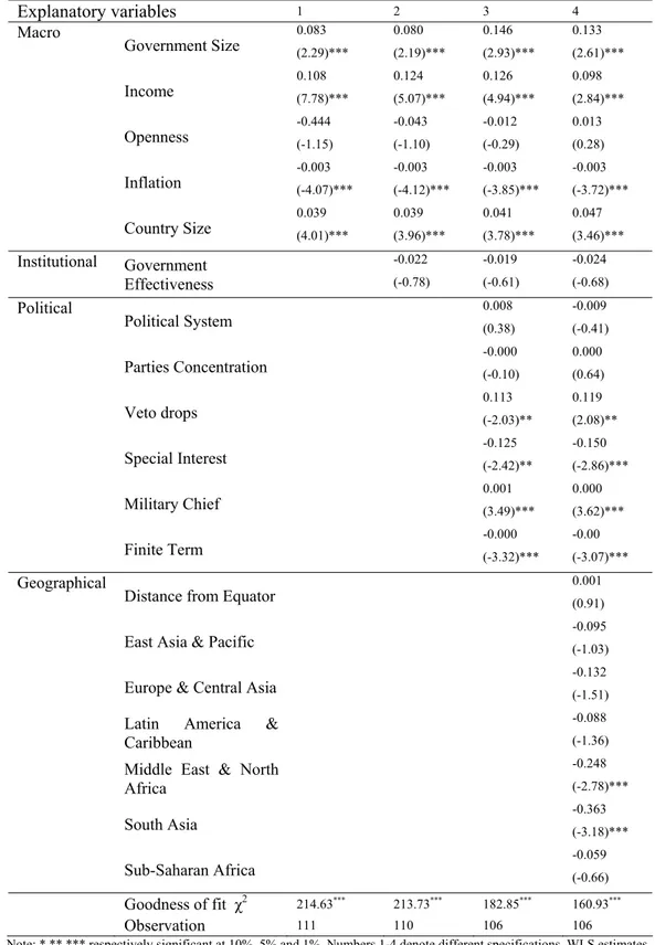
We now proceed to analyze the determinants for persistence of government

spending. In Table 5 we report the results of estimating equation 4. In particular, as we did

for the estimate of our discretion equation, we report four columns each presenting a

different specification of the set of controls.

As already argued, we should expect at least for some of the controls, that if a cross

country covariate has a negative (positive) impact on discretion it should have a positive

(negative) impact on the persistence of government spending. This intuition is confirmed

by our results. In fact, looking at the first column of Table 5, we can see that most of the

macroeconomic variables are statistically significant and they have opposite signs with

respect to the volatility of spending discretion.

However there are exceptions. For example, institutional variables are not

significant in the specification for fiscal persistence but they are significant in the fiscal

discretion specification. Other variables such as military chief and finite term enter with

the same sign in both the persistence and the discretionary equation. In particular, we find

that countries with higher political stability and with a military chief have a more

persistent government spending. In contrast, countries where the executive has a given

finite term or in which the executive represent special interests have a less persistent

government spending.

Given the high correlation between spending and revenue in our sample (0.9) it is

likely to expect that the determinants of discretion and persistence have a similar effect on

spending and revenue. However, as we discussed in section 4.1, government revenue tends

components of discretion and persistence of government revenue are affected in a similar

way by our set of explanatory variables cannot be taken for granted.

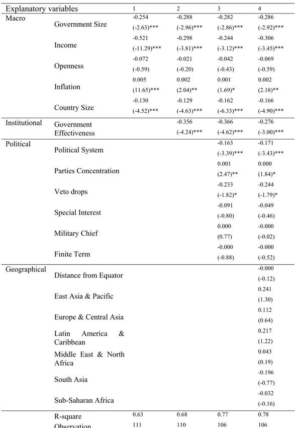
In Table 6 and 7, we report the estimates of equations (3) and (4) for government

revenue. Focusing first on the revenue discretion equation (Table 6), we can observe that

similarly to the volatility of government spending discretion, government size, country

size, income, government effectiveness, parliamentary system and veto drops are

negatively associated with the discretion component of revenue. In contrast, countries with

higher inflation and characterized by lower concentration of parties tend to have more

government revenue discretion.

Analyzing the results for revenue persistence (Table 7) we can see that, as for the

spending specification, macroeconomic variables such as income and country size are

significant and they have opposite sign with respect to the revenue discretion equation. In

contrast, government effectiveness, political stability, parliamentary system and party

concentration have the same sign in both the persistence and discretion equation (Tables 6

and 7). Other variables such as military chief and finite term are only significant in the

persistence specification, and the sign of their coefficients is the same as in the spending

specification.

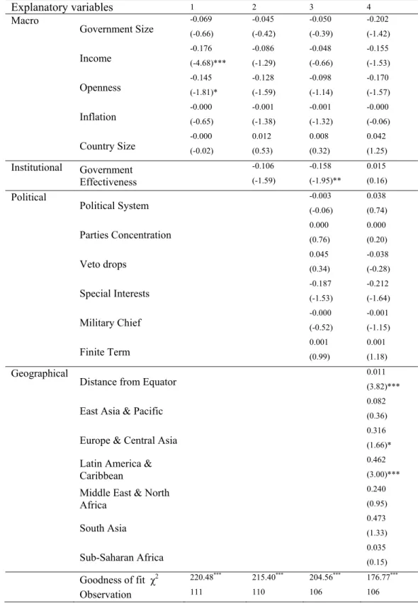
We conclude our analysis by assessing the cross-country determinants of

responsiveness of fiscal policy. In Table 8 we report the results of estimating equation (5)

for government spending. Starting with the first column of the table, we can see that an

only variable that is statistically significant is income. In particular, we find that developed

countries tend to be less pro-cyclical. This result is in line with other evidence in the

literature, as discussed in the previous section of the paper. However, when include the

statically significant. In contrast, as argued by Gavin and Perotti (1997a), we find that

government spending is highly pro-cyclical in Latin America.

Different results are obtained when we estimate equation (5) for government

revenue (Table 9). In particular, we find that while government size, government

effectiveness, special interests, East Asia & Pacific, and Europe & Central Asia dummies

are positively associated with revenue responsiveness, openness is negatively related. This

different behaviour between the responsiveness of government spending and revenue is

coherent with the fact that countries with pro-cyclical (counter-cyclical) spending may not

have necessarily pro-cyclical (counter-cyclical) revenue, and vice versa.

4.3 Robustness Analysis

The behaviour of fiscal policy varies across countries.Thus, it is interesting to see

whether our estimated measures of responsiveness, persistence and discretion are different

across groups of countries. To this purpose, we consider three groups of countries: EMU,

OECD and non OECD countries. Looking at the panel results reported in Table 10, it is

possible to see that the responsiveness of both expenditure and revenue to output is lower

than for the measure of persistence for all set of countries. Moreover, it does not seem that

countries significantly differ in terms of responsiveness. In contrast, country groups

systematically differ in terms of discretion and persistence of both expenditure and

revenue. In particular, EMU countries are those characterized by the lowest estimated

discretion coefficient for spending, while non OECD countries are those with the highest

(lowest) level of discretion (persistence).

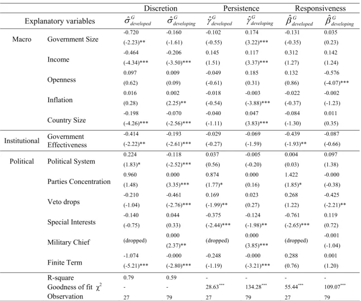
It is also possible to argue that most of the variation in many determinants of

government spending and revenue, and its persistence, responsiveness and discretion

and developing countries. Thus, both from a theoretical perspective and, especially, from a

policy point of view it is important to assess whether our analysis is robust within

developed and developing country grouping. Table 11 reports the results both for the

discretion, persistence and responsiveness equations for government spending. The first

two columns refer to the results relative to fiscal discretion respectively for developed and

developing countries. Looking at these two columns, it seems that there is not much

discrepancy between the two groups. For both sets of countries, spending discretion is

negatively related to GDP per capita, country size, government effectiveness and the

dummy for finite terms. In contrast, other political variables and inflation seem to affect

spending discretion only for developing countries.

The second two columns report the results of the persistence equation for both

developed and developing countries. Differently from what was obtained for the equation

regarding the discretion component, it seems that while macroeconomic variables have

been more relevant for fiscal persistence in developing countries, political and institutional

variables in general played a role in affecting fiscal persistence in both developed and

developing countries, even if with some differences.

Finally, analyzing the last two columns we can see that the determinants of

responsiveness of government spending vary between developed and developing countries.

In particular, while government effectiveness and special interests are essentially the only

variables found to be significant in the specification for developed countries, openness and

veto drops are the only variables that have a statistically significant impact on spending

responsiveness in developing countries. This result suggests that not only the measure of

responsiveness and cyclicality varies between developing and developed countries, but this

is also true for its determinants.

5. Conclusion

By making use of a two-step estimation procedure, we pursue a twofold objective

in this paper. First, we provide an empirical study on the decomposition of fiscal policy

into three components: responsiveness, persistence and discretion. Second, we analyze the

determinants of these components. The key conclusions of our analysis are as follows.

Using a country-specific estimation approach to disentangle the abovementioned

three components of fiscal policy, both for government spending and revenue, we find

that, for most of the 132 countries in our sample, fiscal policy is rather more persistent

than responsive to current economic conditions. More interestingly, we find that, for both

revenue and spending, persistence is negatively correlated to the discretion component

thereby suggesting that countries with higher persistence have lower discretion. The above

conclusions are robust by considering the AMECO dataset for EU countries, for a larger

time span. In the second part of our analysis, we carry out a cross-country estimation

approach to identify the source of fluctuations of persistence, responsiveness and

discretion components. According to the previous empirical finding, suggesting a negative

relationship between discretion and persistence, we find that while government size and

effectiveness and income have negative effects on the discretion component of fiscal

policy, they tend to increase fiscal persistence. Moreover, we find that macro and political

and institutional variables are less relevant for responsiveness, once regional dummies are

considered.

Our study suggests possible extensions. In fact, comparing for each country the

estimates of the degree of persistence from government expenditure and revenue equations

and the starting value of these two series, one could be able to detect signals of potential

fiscal deterioration (some preliminary analysis is provided in Appendix 2).

Afonso, A. (2005). “Fiscal Sustainability: the Unpleasant European Case”, FinanzArchiv,

61 (1), 19-44.

Afonso, A. (2008). “Ricardian Fiscal Regimes in the European Union”, Empirica, 35 (3),

313–334.

Afonso, A. and Rault, C. (2007). “What do we really know about fiscal sustainability in

the EU? A panel data diagnostic”, ECB Working Paper n. 820.

Akitoby, B., Clements, B., Gupta S., and Inchauste, G. (2004). “The cyclical and

long-term behavior of government expenditures in developing countries”, IMF Working

Paper 04.202.

Alesina, A., Campante, F. and Tabellini, G. (2008). “Why is Fiscal Policy Often

Procyclical?” Journal of the European Economic Association, 6(5), forthcoming.

Alesina, A. and Perotti, R. (1994). “The Political Economy of Budget Deficits”, NBER

Working Paper 4637.

Alesina A. and Tabellini G. (2005). “Why is fiscal policy often procyclical?” mimeo, July.

Alesina, A. and Wacziarg, R. (1998). “Openness, country size and government”, Journal

of Public Economics,69 (3), 305-321.

Barlevy G. (2004). “The Cost of Business Cycles and the Benefits of Stabilization: A

Survey”, NBER Working Paper 10926.

Barro R. (1979). “On the Determination of the Public Debt”, Journal of Political

Economy, 87 (5), 93-110.

Braun M. (2001). “Why Is Fiscal Policy Procyclical in Developing Countries”, Harvard

University.

Darby, J. and Melitz, J. (2007). “Labour Market Adjustment, Social Spending and the

Automatic Stabilizers in the OECD”, CEPR Discussion Paper 6230.

Drazen, A. (2000). Political Economy in Macroeconomics, Princeton: Princeton University

Press.

Epaulard, A. and Pommeret, A. (2003). “Recursive Utility, Endogenous Growth, and the

Welfare Cost of Volatility”, Review of Economic Dynamics, 6(3), 672-684.

Fatás, A. and Mihov, I. (2001). “Government Size and Automatic Stabilizers”, Journal of

International Economics, 55, 3-28.

Fatás, A. and Mihov, I. (2003). “The Case for Restricting Fiscal Policy Discretion”,

QuarterlyJournal of Economics, 118, 1419-1447.

Fatás, A. and Mihov, I. (2005). “Policy volatility, institutions and economic growth”,

Fatás, A. and Mihov, I. (2006). “The Macroeconomics Effects of Fiscal Rules in the US

States”, Journal of Public Economics, 90, 101-117.

Ferejohn. (1986). “Incumbent performance and electoral control”, Public Choice 30, 5-25.

Fiorito R. (1997). “Stylized Facts of Government Finance in the G-7”, IMF Working

Paper 97/142.

Fiorito R. and Kollintzas T. (1994). “Stylized Facts of Business Cycles in the G7 from a

Real Business Cycles Perspective”, European Economic Review, Vol. 38, pp. 235-69.

Furceri, D. (2007). “Is Government Expenditure Volatility Harmful for Growth? A

Cross-country Analysis”, Fiscal Studies, 28 (1), 103-120.

Furceri, D., and Poplawski, M. (2008). “Fiscal Volatility and the size of Nations”, Mimeo.

Gali J. (1994). “Government Size and Macroeconomic Stability”, European Economic

Review, 38 (1), 117-32.

Galí J. (2005). “Modern perspective of fiscal stabilization policies”, CESifo Economic

Studies, 51 (4), 587-599.

Galí J. and Perotti R. (2003). “Fiscal policy and monetary integration in Europe”, Fiscal

Policy, 533-572 (October).

Gavin M. and Perotti R. (1997a). “Fiscal policy in Latin America”, NBER

Macroeconomics Annual, (12), 11-71.

Gavin M. and Perotti R. (1997b). “Fiscal policy and saving in good times and bad times”,

in Hausman R., Reisen H. (Eds.), Promoting Savings in Latin America, IDB and

OECD.

Hallerberg, M. and Strauch, R. (2002). “On the Cyclicality of Fiscal Policy in Europe”,

Empirica, 29, 183-207.

Imbs, J. (2007). “Growth and volatility”, Journal of Monetary Economics, 54 (7),

1848-1862.

Kaminsky, G., Reinhart, C. and Végh, C. (2004). “When It Rains, It Pours: Procyclical

Capital Flows and Macroeconomic Policies”, NBER Working Paper 10780.

Lane, P. (2003). “The cyclical behaviour of fiscal policy: evidence from the OECD”,

Journal of Public Economics, 87 (12), 2261-2675.

La Porta, R., Lopez de Silanes, F., Shleifer, A. and Vishny, R. (1998). “The Quality of

Government”, Journal of Law, Economics and Organization, 15 (1), 222-279.

Persson, T. (2001). “Do Political Institutions Shape Economic Policy?” NBER Working

Persson, T. and Tabellini, G. (2001). “Political Institutions and Policy Outcomes: What are

the Stylized Facts ? ” CEPR Discussion Papers 2872.

Ramey and Ramey (1995). “Cross-Country Evidence on the Link between Volatility and

Growth”, American Economic Review, 85 (5), 1138-51.

Rand, J., and Tarp, F. (2002). “Business cycles in developing countries: Are they

different?” World Development, 30 (12), 2071-2088.

Rodrick, D. (1998). “Why Do More Open Economies Have Bigger Governments?”

Journal of Political Economy, 106 (5), 997-1032.

Sorensen, B., Wu, L. and Yosha, O. (2001). “Output fluctuations and fiscal policy: U.S.

state and local governments 1978–1994”, European Economic Review, 45, 1271-310.

Talvi E. and Vegh, C. (2005). “Tax base variability and procyclical fiscal policy”, Journal

Figure 1. Scatter plot ofγˆ vs._iG G i

σˆ from country-specific spending equation.

AGO ALB ARE ARG AUS AUT BDI BEL BFA BGR BHS BLZ BOL BRA BRB BRN BTN BWA CAF CAN CHE CHL CHN CIV CMR COG COL COM CPV CRI CYP CZE DEU DMA DNK DOM ECU EGY ESP ETH FIN FRA GBR GIN GMB GNB GNQ GRC GUY HKG HTI HUN IDN IND IRL _IRN ISL ISR ITA JAM JOR JPN KEN KHM KIR KOR KWT LAO LBN LBY LCA LKA LSO LUX MAR MDG MDV MEX MLI MLT MMR MOZ MRT MUS MWI MYS NER NGA NIC NLD NOR NZL OMN PAK PAN PER PHL POL PRTPRY QAT ROM

SEN SGP SLE

SLV STP SUR SWE SWZ SYC SYR TCD TGO THA TON TTO TUN TUR

TWN TZA _UGA

URY USA VCT VEN VNM VUT WSM ZAF ZMB ZWE -1 -. 5 0 .5 1 gam m a (G)

-5 -4 -3 -2 -1

log sigma (G)

Figure 2. Scatter plot of R i

γˆ vs. R i

σˆ from country-specific revenue equation.

AGO ALB ARE ARG AUS AUT BDI BEL BFA BGR BHS BLZ BOL BRA BRB BRN BTN BWA CAF CAN CHE CHL CHN CIV CMR COG COL COM CPV CRI CYP CZE DEU DMA DNK DOMECU EGY ESP ETH FIN FRA GBR GIN GMB GNB GNQ GRC GUY HKG HTI HUN IDN IND IRL IRN ISL ISR ITA JAM JOR JPN KEN KHM KIR KOR KWT LAO LBN LBY LCA LKA LSO LUX MAR MDG MDV MEX MLI MLT MMR MOZ MRT MUS MWI MYS NER NGA NIC NLD

NOR NZLOMN

PAK PAN PER PHL POL PRT PRY QAT ROM SEN SGP SLE SLV STP SUR SWE _SWZ SYC SYR TCD TGO THA TON TTO TUN TUR TWN TZA UGA URY USA VCT VEN VNM VUTWSM ZAF ZMB ZWE -1 .5 -1 -. 5 0 .5 1 ga m m a ( R )

-5 -4 -3 -2 -1 0

Table 1. Estimates of Responsiveness (β), Persistence (γ) and Discretion (σ)

parameter estimates (1980-2007) parameter estimates (1980-2007)

country βG βR γG γR σG σR country βG βR γG γR σG σR

Angola 0.02 0.07 -0.29 0.56** 0.16 0.19 Kuwait -0.01 1.21*** 0.6*** 0.29** 0.09 0.12

Albania 0.92 -0.5 0.63** 0.69 0.06 0.22 Lao PDR -0.77 2.71** -0.27 -0.11 0.14 0.14

United Arab

Emirates 1.74** 2.38 0.04 0.14 0.09 0.15 Lebanon -0.26 1.31 0.94*** -0.04 0.18 0.23

Argentina 1.48** 1.22 0.11 0.13 0.13 0.10 Libya 0.24 -0.47 0.54* 0.34 0.12 0.13

Australia 0.36 2.17*** 0.81*** 0.49*** 0.03 0.03 St. Lucia 0.35 0.98** 0.38** -0.08 0.08 0.07

Austria -0.05 2.1*** 0.75*** -0.12 0.02 0.03 Sri Lanka 0.78 0.05 0.3* 0.7*** 0.05 0.05

Burundi 1.49*** 2.83*** 0.06 -0.12 0.11 0.11 Lesotho 0.16 0.45 0.5*** 0.76** 0.09 0.08

Belgium -0.42 -0.38 -0.1 0.57*** 0.02 0.02 Luxembourg 0.66* 0.37 0.56** 0.44* 0.05 0.04

Burkina Faso 2.29 -0.71 -0.38 -0.19 0.12 0.22 Morocco 0.28 1.73** 0.51** 0.47** 0.05 0.07

Bulgaria 1.3*** 2.15*** 0.09 -0.23 0.06 0.07 Madagascar -2.93 23.26 0.18 -1.51 0.19 0.69

Bahamas -0.02 0.11 -0.02 0.47* 0.04 0.05 Maldives 1.32 3.27 0.15 0.22 0.13 0.22

Belize 1.5*** 0.02 0.22 0.79 0.09 0.10 Mexico 0.86 -0.2 0.19 0.19 0.18 0.15

Bolivia 1.79 -1.05 0.09 0.16 0.09 0.28 Mali -0.22 -0.74 0.3 -0.12 0.08 0.22

Brazil 0.52 -0.62 0.63 0.47 0.10 0.09 Malta 0.39 0 0.55* 0.65** 0.07 0.07

Barbados 0.83** 0.41** 0.33 0.24 0.07 0.03 Myanmar 1.21*** 0.57 -0.02 0.36* 0.10 0.13

Brunei 2.83 8.61 -0.01 0.06 0.10 0.16 Mozambique 1.22** 1.44** 0.4*** 0.62*** 0.14 0.16

Bhutan 0.3 0.23 0.24 0.23 0.14 0.13 Mauritania -2.61 -3.05 0.75*** 0.17 0.16 0.31

Botswana 0.98** 0.33 0.24 0.64*** 0.06 0.09 Mauritius 0.33 -1.14 0.6*** 0.81* 0.05 0.07

Central African

Republic 0.04 0.3 0.32** 0.24 0.17 0.23 Malawi 2.46* 3.65 -0.75 -0.35 0.20 0.23

Canada 0.18 0.38** 0.91*** 0.44** 0.02 0.02 Malaysia -0.04 0.76** 0.11 0.23 0.05 0.06

Switzerland -0.97 0.11 0.55** 0.36*** 0.02 0.02 Niger -0.16 1.99* 0.66 -0.17 0.15 0.24

Chile 0.31 0 0.77*** 0.29* 0.04 0.05 Nigeria 0.24 0.84 0.51* 0.55*** 0.25 0.20

China 1.32*** 1.32*** 0.97*** 0.93*** 0.04 0.04 Nicaragua 3.37** 3.09** 0.18 0.23 0.17 0.17

Cote d'Ivoire 0.09 0.34 0.64*** 0.79*** 0.08 0.08 Netherlands 0.81 0.69* 1.09*** 0.59*** 0.02 0.03

Cameroon 1.39*** 2.61*** 0.09 -0.27 0.09 0.20 Norway -0.92*** 0.99*** 0.27 0.55*** 0.02 0.02

Congo, Rep. 2.21** 1.08* 0.18 0.15 0.13 0.09 New Zealand 0.22 -0.49 0.79** 0.62** 0.05 0.05

Colombia 1.54*** 0.91*** 0.61*** 0.42** 0.05 0.04 Oman 0.47 0.64** 0.47** 0.59*** 0.05 0.05

Comoros 5.65 7.27 0.28 0.27 0.16 0.17 Pakistan 1.78 0.72 0.4 0.67** 0.06 0.06

Cape Verde -1.26 -0.51 0.8*** 0.58*** 0.14 0.10 Panama 0.39 0.63 0.27 0.22 0.06 0.10

Costa Rica 0.66 -0.64 -0.09 0.1 0.11 0.15 Peru -0.59 -1.16** 1.07* 0.77*** 0.12 0.16

Cyprus 0.17 -0.38 0.35** 0.58 0.04 0.04 Philippines -0.09 -0.49 0.59*** 0.94*** 0.07 0.08

Czech Republic 1.11*** 1.63*** 0.62*** 0.4** 0.04 0.04 Poland 0.75*** 0.34 0.34*** 0.65** 0.04 0.05

Germany 0.8*** 0.85*** 0.44*** 0.38*** 0.02 0.01 Portugal 0.41 0.28 0.47** 0.49** 0.07 0.07

Dominica 0.24 -0.77 0.51*** 0.75** 0.07 0.09 Paraguay 1.37*** 1.87*** 0.54*** 0.44** 0.08 0.06

Denmark -0.55** 0.77** 0.85*** 0.37** 0.01 0.02 Qatar 0.5 0.47* 0.33* 0.2 0.10 0.12

Dominican Republic 1.26* 0.15 0.4 0.28 0.12 0.12 Romania 0.52 0.58 0.54*** 0.59*** 0.06 0.07

Ecuador 4.48 0.33 0.31 0.34 0.17 0.15 Senegal 2.19*** 1.15* 0.34* 0.45 0.07 0.05

Egypt, Arab Rep. 1.78*** 0.17 0.31 0.48** 0.11 0.10 Singapore 2.92** 2.73 0.39 0.17 0.12 0.10

Spain 0.61*** 0.71*** 0.9*** 0.73*** 0.02 0.02 Sierra Leone 0.57 1.14 0.4** 0.3 0.21 0.28

Ethiopia 2.73*** 1.5 0.45*** 0.58* 0.13 0.12 El Salvador 1.58** 2.72*** 0.75*** 0.85*** 0.10 0.11 Finland 0.02 0.6*** 0.85*** 0.47*** 0.03 0.03 Sao Tome and Principe 2.14 5.99* 0.36 0.11 0.25 0.43

France 0.45* -0.07 1.07*** 0.71*** 0.01 0.01 Suriname 0.36 0.08 0.22 0.13 0.10 0.14

United Kingdom -0.16 0.82 0.76*** 0.51** 0.02 0.02 Sweden -0.21 0.94*** 0.68*** 0.32 0.02 0.02

Guinea 4.22 3.55 0.24 0.21 0.15 0.15 Swaziland 0.48 1.24*** 0.5*** 0.29** 0.08 0.06

Gambia, The -0.79 -1.68 -0.12 0.58*** 0.12 0.16 Seychelles 1.27*** -0.44 0.02 0.83*** 0.07 0.07

Guinea-Bissau 0.48 -0.04 -0.03 -0.02 0.17 0.29 Syrian Arab Republic 0.11 0.93 0.64*** 0.32* 0.08 0.09

Equatorial Guinea 0.23 0.47** 0.52*** 0.4** 0.27 0.27 Chad -0.05 0.78 0.55*** 0.77*** 0.14 0.18

Greece 0.2 -0.7 0.39 0.88*** 0.04 0.04 Togo 0.3 -0.18 0.55*** 0.56 0.11 0.22

Guyana -0.21 0.15 0.63*** 0.06 0.13 0.14 Thailand 0.78*** 1.65*** 0.91*** -0.21 0.06 0.05

Table 1 (contd.). Estimates of Responsiveness (β), Persistence (γ) and Discretion (σ)

parameter estimates (1980-2007) parameter estimates (1980-2007)

country βG βR γG γR σG σR country βG βR γG γR σG σR

Haiti -3.74 -5.82 0.97*** 0.93*** 0.28 0.36 Trinidad and Tobago 1.09*** 0.55** 0.27 0.27 0.06 0.06

Hungary 0.23 1.42*** 0.71*** 0.15 0.04 0.03 Tunisia 2.06 3.72 0.04 0.13 0.06 0.08

Indonesia 0 0.33 0.25 0.18 0.09 0.06 Turkey 0.06 0.28 0.4 0.14 0.09 0.08

India 1.23** 0.63** 0.28* -0.07 0.03 0.03 Taiwan 1.75* 1.38 0.19 -0.01 0.07 0.05

Ireland 0.26 0.31* 0.51*** 0.33* 0.03 0.03 Tanzania 0.95 0.85 0.23 0.04 0.11 0.09

Iran, Islamic Rep. 0.57 0.51 0.48** 0.64** 0.15 0.17 Uganda 1.28 2.02* 0.16 0.08 0.17 0.18

Iceland 0.56** 0.82*** 0.63*** 0.32** 0.03 0.03 Uruguay 0.84*** 1.05** 0.47** 0.41* 0.05 0.06

Israel 0.77*** 0.33 0.48*** 0.37* 0.02 0.05 United States 0.27 1.05*** 0.83*** 0.51** 0.01 0.03

Italy 1.15*** 0.68* 0.81*** 0.8*** 0.02 0.02

St. Vincent and the

Grenadines -0.07 -1.31 0.58* 0.59* 0.09 0.08

Jamaica -1.1 -1.24 0.4** 0.57** 0.07 0.10 Venezuela, RB 1.07 -0.29 -0.04 0.63 0.11 0.11

Jordan 0.42 0.07 0.36 0.24 0.11 0.09 Vietnam -1.15 -1.27 0.28 0.83*** 0.14 0.10

Japan 0.4** 1.1*** 0.83*** 0.42 0.02 0.03 Vanuatu 0.95 1.21** 0.47** 0.35** 0.13 0.12

Kenya 0.96** 0.47* 0.26 0.62*** 0.08 0.05 Samoa -1.4 0.37 0.49** 0.36* 0.10 0.14

Cambodia -11.96* -9.63** -0.72 -0.37 0.22 0.27 South Africa -0.59 0.69* 0.68*** 0.49** 0.03 0.03

Kiribati 0.97** 0.15 0.14 0.25 0.14 0.18 Zambia 0.9 -0.27 0.3 -0.21 0.11 0.14

Korea, Rep. 0.25 0.03 0.88*** 0.51*** 0.04 0.04 Zimbabwe 0.08 -0.35 0.63* 0.88*** 0.16 0.13

Notes: E – expenditure; R – revenue. *, ***, ***, significant at respectively 10, 5, and 1 per cent.

Table 2. Spearman correlation matrix

γG _γR _σG _σR

γG

1

γR

0.395 1

σG

-0.391 -0.279 1 σR

-0.388 -0.309 0.900 1

Table 3. Results with AMECO dataset

parameter estimates (1960-2007)

country βˆG βˆR γˆG γˆR σˆG σˆR

Austria 0.59*** 0.52** 0.78*** 0.76*** 0.02 0.02

Belgium 0.97*** 0.39* 0.66*** 0.79*** 0.03 0.01

Germany 0.51** 0.42* 0.73*** 0.73*** 0.02 0.03

Denmark 0.36 1.15* 0.90*** 0.68*** 0.03 0.04

Spain 0.28* 0.39 0.99*** 0.93*** 0.02 0.03

Finland 0.24* 0.39*** 0.93*** 0.80*** 0.04 0.04

France 0.06 -0.15 0.90*** 1.03*** 0.01 0.02

United Kingdom 0.47* 0.54** 0.85*** 0.81*** 0.04 0.03

Greece 0.08 0.16 0.88*** 0.77*** 0.04 0.03

Ireland -0.01 -0.02 0.69*** 0.65*** 0.04 0.03

Italy 0.59*** 0.14 0.75*** 0.89*** 0.02 0.03

Netherlands 0.46*** 0.55*** 0.85*** 0.81*** 0.02 0.02

Portugal 0.44*** 0.5*** 0.86*** 0.67*** 0.04 0.04

Sweden -0.39 0.03 0.77*** 0.79*** 0.03 0.03

United States 0.28 0.76*** 0.83*** 0.59*** 0.02 0.02

Japan 0.32*** 0.27*** 0.77*** 0.78*** 0.04 0.03

Table 4. Determinants of Spending Discretion (σˆ_iG)

Explanatory variables 1 2 3 4

Macro Government Size -0.198 (-2.49)*** -0.206 (-2.69)*** -0.177 (-2.00)** -0.180 (-1.86)* Income -0.497 (-12.48)*** -0.298 (-5.72)*** -0.262 (-5.06)*** -0.332 (-5.44)*** Openness 0.016 (0.15) 0.072 (0.76) 0.094 (0.93) 0.089 (0.78) Inflation 0.005 (7.85)*** 0.002 (3.23)*** 0.002 (1.92)* 0.002 (3.27)*** Country Size -0.103 (-4.54)*** -0.090 (-4.27)*** -0.103 (-4.50)*** -0.091 (-3.05)***

Institutional _Government Effectiveness -0.327 (-5.32)*** -0.326 (-5.73)*** -0.192 (-2.42)** Political Political System -0.135 (-2.85)*** -0.100 (-1.93)* Parties Concentration 0.001 (3.99)*** 0.000 (2.22)** Veto drops -0.191 (-1.62) -0.194 (-1.52) Special Interest 0.072 (0.60) 0.127 (1.13) Military Chief 0.001 (3.90)*** 0.000 (1.81)* Finite Term -0.000 (-2.81)*** -0.000 (-2.25)** Geographical

Distance from Equator

0.000

(0.01)

East Asia & Pacific

0.333

(1.94)*

Europe & Central Asia

0.074

(0.47)

Latin America & Caribbean

0.470

(2.48)**

Middle East & North Africa 0.279 (1.22) South Asia -0.028 (-0.14) Sub-Saharan Africa 0.113 (0.66)

R-square 0.67 0.73 0.78 0.82

Observations 111 110 106 106

Table 5. Determinants of Spending Persistence (γˆ_iG)

Explanatory variables 1 2 3 4

Macro Government Size 0.083 (2.29)*** 0.080 (2.19)*** 0.146 (2.93)*** 0.133 (2.61)*** Income 0.108 (7.78)*** 0.124 (5.07)*** 0.126 (4.94)*** 0.098 (2.84)*** Openness -0.444 (-1.15) -0.043 (-1.10) -0.012 (-0.29) 0.013 (0.28) Inflation -0.003 (-4.07)*** -0.003 (-4.12)*** -0.003 (-3.85)*** -0.003 (-3.72)*** Country Size 0.039 (4.01)*** 0.039 (3.96)*** 0.041 (3.78)*** 0.047 (3.46)***

Institutional _Government Effectiveness -0.022 (-0.78) -0.019 (-0.61) -0.024 (-0.68) Political Political System 0.008 (0.38) -0.009 (-0.41) Parties Concentration -0.000 (-0.10) 0.000 (0.64) Veto drops 0.113 (-2.03)** 0.119 (2.08)** Special Interest -0.125 (-2.42)** -0.150 (-2.86)*** Military Chief 0.001 (3.49)*** 0.000 (3.62)*** Finite Term -0.000 (-3.32)*** -0.00 (-3.07)*** Geographical

Distance from Equator

0.001

(0.91)

East Asia & Pacific

-0.095

(-1.03)

Europe & Central Asia

-0.132

(-1.51)

Latin America & Caribbean

-0.088

(-1.36)

Middle East & North Africa -0.248 (-2.78)*** South Asia -0.363 (-3.18)*** Sub-Saharan Africa -0.059 (-0.66)

Goodness of fit χ2 214.63*** _213.73*** _182.85*** _160.93***

Observation 111 110 106 106

Table 6. Determinants of Revenue Discretion (σˆ_iR)

Explanatory variables 1 2 3 4

Macro Government Size -0.254 (-2.63)*** -0.288 (-2.96)*** -0.282 (-2.86)*** -0.286 (-2.92)*** Income -0.521 (-11.29)*** -0.298 (-3.81)*** -0.244 (-3.12)*** -0.306 (-3.45)*** Openness -0.072 (-0.59) -0.021 (-0.20) -0.042 (-0.43) -0.069 (-0.59) Inflation 0.005 (11.65)*** 0.002 (2.04)** 0.001 (1.69)* 0.002 (2.18)** Country Size -0.130 (-4.52)*** -0.129 (-4.63)*** -0.162 (-6.33)*** -0.166 (-4.90)***

Institutional _Government Effectiveness -0.356 (-4.24)*** -0.366 (-4.62)*** -0.276 (-3.00)*** Political Political System -0.163 (-3.39)*** -0.171 (-3.43)*** Parties Concentration 0.001 (2.47)** 0.000 (1.84)* Veto drops -0.233 (-1.82)* -0.244 (-1.79)* Special Interest -0.091 (-0.80) -0.049 (-0.46) Military Chief 0.000 (0.77) -0.000 (-0.02) Finite Term -0.000 (-0.88) -0.000 (-0.52) Geographical

Distance from Equator

-0.000

(-0.12)

East Asia & Pacific

0.241

(1.30)

Europe & Central Asia

0.112

(0.64)

Latin America & Caribbean

0.217

(1.22)

Middle East & North Africa 0.043 (0.19) South Asia -0.196 (-0.77) Sub-Saharan Africa -0.032 (-0.16)

R-square 0.63 0.68 0.77 0.78

Observation 111 110 106 106

Table 7. Determinants of Revenue Persistence (γˆ_iR)

Explanatory variables 1 2 3 4

Macro Government Size 0.063 (1.62)* 0.064 (1.66)* 0.098 (1.96)** 0.067 (1.28) Income 0.021 (1.32) 0.069 (2.36)** 0.068 (2.28)** 0.066 (1.62)* Openness 0.023 (0.50) 0.018 (0.39) 0.113 (2.23)** 0.059 (0.98) Inflation -0.000 (-0.20) -0.000 (-1.03) -0.000 (-0.94) -0.000 (-0.67) Country Size 0.039 (3.85)*** 0.040 (3.89)*** 0.045 (4.03)*** 0.052 (3.49)***

Institutional _Government Effectiveness -0.063 (-1.95)** -0.027 (-0.71) -0.002 (-0.05) Political Political System -0.071 (-2.71)*** -0.060 (-2.10)** Parties Concentration 0.000 (2.55)*** 0.000 (2.73)*** Veto drops 0.184 (3.00)*** 0.184 (2.93)*** Special Interests -0.008 (-0.16) -0.031 (-0.57) Military Chief 0.001 (2.89)*** 0.000 (2.64)*** Finite Term -0.000 (-2.89)*** -0.000 (-2.94)*** Geographical

Distance from Equator

0.004

(3.42)***

East Asia & Pacific

0.102

(0.98)

Europe & Central Asia

-0.109

(-0.94)

Latin America & Caribbean

0.016

(0.20)

Middle East & North Africa 0.002 (0.02) South Asia -0.210 (-1.67)* Sub-Saharan Africa 0.088 (0.77)

Goodness of fit χ2 254.04*** 250.07*** 219.30*** 195.74***

Observation 111 110 106 106

Table 8. Determinants of Spending responsiveness ( G i

βˆ ₎

Explanatory variables 1 2 3 4

Macro Government Size -0.069 (-0.66) -0.045 (-0.42) -0.050 (-0.39) -0.202 (-1.42) Income -0.176 (-4.68)*** -0.086 (-1.29) -0.048 (-0.66) -0.155 (-1.53) Openness -0.145 (-1.81)* -0.128 (-1.59) -0.098 (-1.14) -0.170 (-1.57) Inflation -0.000 (-0.65) -0.001 (-1.38) -0.001 (-1.32) -0.000 (-0.06) Country Size -0.000 (-0.02) 0.012 (0.53) 0.008 (0.32) 0.042 (1.25)

Institutional _Government Effectiveness -0.106 (-1.59) -0.158 (-1.95)** 0.015 (0.16) Political Political System -0.003 (-0.06) 0.038 (0.74) Parties Concentration 0.000 (0.76) 0.000 (0.20) Veto drops 0.045 (0.34) -0.038 (-0.28) Special Interests -0.187 (-1.53) -0.212 (-1.64) Military Chief -0.000 (-0.52) -0.001 (-1.15) Finite Term 0.001 (0.99) 0.001 (1.18) Geographical

Distance from Equator

0.011

(3.82)***

East Asia & Pacific

0.082

(0.36)

Europe & Central Asia

0.316

(1.66)*

Latin America & Caribbean

0.462

(3.00)***

Middle East & North Africa 0.240 (0.95) South Asia 0.473 (1.33) Sub-Saharan Africa 0.035 (0.15)

Goodness of fit χ2 220.48*** _215.40*** _204.56*** _176.77***

Observation 111 110 106 106

Table 9. Determinants of Revenue responsiveness ( R i

βˆ ₎

Explanatory variables 1 2 3 4

Macro Government Size 0.219 (1.95)** 0.206 (1.78)* 0.413 (3.18)*** 0.235 (1.63)* Income -0.011 (-0.28) 0.014 (0.21) -0.025 (-0.33) 0.006 (0.06) Openness -0.028 (-0.31) -0.031 (-0.34) -0.060 (-0.62) -0.395 (-3.19)*** Inflation -0.002 (-1.96)** -0.002 (-1.92)** -0.003 (-2.40)** -0.002 (-1.26) Country Size 0.000 (0.04) -0.003 (-0.12) 0.003 (0.10) -0.049 (-1.44)

Institutional _Government Effectiveness -0.032 (-0.48) 0.045 (0.49) 0.214 (2.09)** Political Political System -0.023 (-0.43) -0.053 (-0.89) Parties Concentration -0.000 (-2.03)** -0.000 (-1.74)* Veto drops 0.089 (0.69) 0.081 (0.61) Special Interests 0.317 (2.65)*** 0.275 (2.20)** Military Chief 0.000 (0.25) -0.000 (-0.25) Finite Term 0.000 (0.49) 0.000 (0.78) Geographical

Distance from Equator

0.009

(2.56)***

East Asia & Pacific

0.770

(3.30)***

Europe & Central Asia

0.906

(3.75)***

Latin America & Caribbean

0.050

(0.30)

Middle East & North Africa 0.345 (1.46) South Asia 0.259 (0.84) Sub-Saharan Africa 0.334 (1.26)

Goodness of fit χ2 262.78*** _262.32*** _237.07*** _212.55***

Observation 111 110 106 106