M
ESTRADO
E
CONOMIA
M
ONETÁRIA E
F
INANCEIRA
T
RABALHO
F
INAL DE
M
ESTRADO
D
ISSERTAÇÃO
RESPONSES OF INFLATION AND OUTPUT TO MONETARY SHOCKS IN
A BAUMOL-TOBIN MODEL
THOMAS JOEL VERHEIJ
M
ESTRADO EM
E
CONOMIA
M
ONETÁRIA E
F
INANCEIRA
T
RABALHO
F
INAL DE
M
ESTRADO
D
ISSERTAÇÃO
RESPONSES OF INFLATION AND OUTPUT TO MONETARY SHOCKS IN
A BAUMOL-TOBIN MODEL
THOMAS JOEL VERHEIJ
O
RIENTAÇÃO
:
B
ERNARDINO
A
DÃO
,
B
ANCO DE
P
ORTUGAL
Responses of In‡ation and Output to Monetary
Shocks in a Baumol-Tobin Model
Thomas Verheij
yInstituto Superior de Economia e Gestão,
Universidade Técnica de Lisboa
Banco de Portugal
Supervisor: Bernardino Adão
Banco de Portugal
27th September 2012
I am very grateful to Bernardino Adão for all his support and comments. I am also very grateful
to Banco de Portugal for providing all the necessary conditions, within the program “Estágios
MEMF – Banco de Portugal”, to make this dissertation possible. I thank Isabel Horta Correia,
André Silva and Pedro Teles for their comments. I also thank Miguel Seixas and Gerrit Verheij
for their very usefull suggestions.
Abstract
The question of how monetary policy a¤ects the main economic variables
remains one of the most important questions of the economic literature. With
this dissertation I will try to contribute to the literature to answer this
ques-tion. I will create a general equilibrium model with market segmentation
based on the model of Alvarez et al (2009). The agents of the model will
make transactions between money and bonds every N periods. The money is
needed to buy goods but does not receive interest. The novelty of my model
is that production will be endogenous. I will introduce a shock to the
nom-inal interest rate and obtain the responses of in‡ation and output. The main
conclusions are twofold. In the …rst place, I obtain that the shock to the
nominal interest rate has real e¤ects because in‡ation responds sluggishly. In
the second place, I obtain that the response of in‡ation changes signi…cantly
when production is endogenous instead of exogenous.
JEL Codes: E3, E4, E5
Keywords: cash-in-advance models, market segmentation, interest rate
Contents
1 Introduction 1
1.1 Literature . . . 2
1.2 Main results . . . 4
2 The model 5 2.1 Households . . . 6
2.2 Firms . . . 15
2.3 Government . . . 16
3 Steady State Equilibrium 16 3.1 Clearing Conditions . . . 16
3.2 Steady State . . . 17
3.3 Calibration . . . 19
3.4 Results . . . 19
4 Monetary Policy Shock 21 4.1 Solution Method . . . 22
4.2 Results . . . 27
5 Conclusion 33
1
Introduction
The question of how monetary policy a¤ects the main economic variables remains one of the most important questions of the economic literature. Since Hume (1752) and Wicksell (1898) has there been written about money, prices and the e¤ect of monetary policy on these variables. Today it is widely accepted that monetary policy is neutral in the long run. This means that it does not a¤ect real economic variables in the long run. There also exist some consensus that monetary policy can a¤ect real variables in the short run. However the way the main marcoeconomic variables respond in the short run to monetary policy is a question to which still does not exist one unique answer.1 With this dissertation I will try to contribute to
the literature to answer this question.
The conventional way to try to understand the response of the main macroeco-nomic variables to monetary policy is to create a general equilibrium model where monetary policy is represented by a shock to some monetary variable. Today it is usually to identify a monetary policy shock as a shock to the nominal interest rate, instead of using a shock to the money supply. To be able to obtain some short run real response of the economy mainly two types of models are used in the literature. The …rst type of models is based on nominal rigidities. The second type are models including market segmentation. This dissertation will be part of the second type of literature.
I will create a general equilibrium model with market segmentation based on the model of Alvarez et al (2009). The main goal of my dissertation is to analyze the
strength of the results presented by them. The main di¤erence between the model I use and the model of Alvarez et al (2009) is that here production will be endogenous, while they use an endowment economy. This way I will try to understand in which way making production endogenous changes the response of in‡ation to monetary policy in this type of models. I also analyze how output is a¤ected by monetary policy in a model with market segmentation. Further, I use a di¤erent and simple, non linear way to solve the equilibrium response of the model to the shock of the nominal interest rate.
My dissertation will be organized in the following way. In the rest of the …rst section I will introduce the literature used for my dissertation and present the main results of this dissertation. In the second section I introduce the model, explaining the behavior of the agents of the model; the households, the …rms and the govern-ment. In the thirth section I present the steady state equilibrium of the model. I will explain the calibration used and show the behavior of the agents in the steady state of the economy. The forth section is about the monetary policy shock. I will explain the method used to solve the equilibrium response of the model to the shock and present the response of the main variables in an endowment economy and in a production economy. Finally, I will conclude in section …ve.
1.1
Literature
consumption. So the agents need to withdraw cash, which has a transaction cost. This way, the main conclusion of these papers is that because …nancial transactions have a cost it will not be optimal for the agents to withdraw cash every period, i.e, …nancial transactions will be made infrequently.
Later, Grossman and Weiss (1983) and Rotemberg (1984) create a general equi-librium model based on the Baumol-Tobin framework. In their models their exist two types of agents; one that makes …nancial transactions in the even periods, and another that only makes …nancial transactions in the odd periods. Their market segmentation is exogenous and not a result of an endogenous optimization process because they simply assume the existence of two types of agents. They analyze the steady state e¤ects of open-market operations in an endowment economy. The main result of their work is that in their models an open-market operations has real e¤ects.
In my model the market segmentation will be exogenously imposed, as in the Grossman-Weiss-Rotemberg framework. A next step would be to introduce the time between two transactions of the …nancial assets into the optimization decision, this means making the market segmentation endogenous. This creates additional di¢-culties to solve the model and lies behind the goal of this dissertation. However their exist some literature using general equilibrium models with endogenous market seg-mentation. Silva (2012), for example, creates a model where agents can choose when they make a transaction between their …nancial assets. He analyses what happens to the welfare cost of in‡ation and concludes that exogenous market segmentation underestimates the welfare cost of in‡ation.
1.2
Main results
The main results of my dissertation are twofold. In the …rst place, I obtain the well known result that in‡ation responds sluggishly to an exogenous shock of the nominal interest rate. This way monetary policy can a¤ect the real interest rate in the short run and, consequently, consumption, labor supply and output. So, I can conclude that market segmentation can be important to explain the way monetary policy a¤ects output and in‡ation. It is important to point out that prices are fully ‡exible in my model and that all the real e¤ects of the monetary policy shock result from the market segmentation.
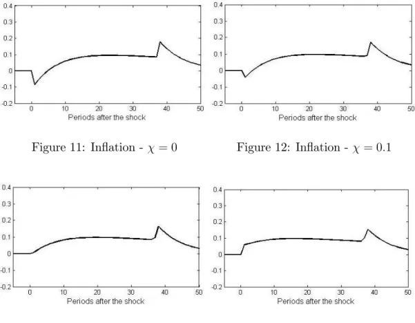
dif-ferent from the response of in‡ation in an endowment economy. I …rst analyze the response of in‡ation in an endowment economy and I obtain the same results as Alvarez et al (2009). During the …rst months after the shocks in‡ation decreases and only after around six months in‡ation starts to increase, turning back to his steady state value after around four years. Now by letting the agents reallocate their labor supply after the shocks, which means making production endogenous, I obtain a di¤erent response of in‡ation to the interest rate shock. Now, instead of decreasing, in‡ation starts to increase right after the shock.
2
The model
payment.2
As mentioned before, the market segmentation in my model is exogenously im-posed. This means that I impose that each agent only makes a transaction between his …nancial assets every N periods. Again, this is not a result of an endogenous optimization process so that the agents can not rearrange the time between two …nancial transactions after the interest rate shock. However this is an ad-hoc as-sumption, one could argue that small monetary shocks will not have much e¤ect on the time between two …nancial transactions. So, in the model their will existN
types of agents and every period only a fraction of N1 of the agents will visit the asset market to make a transaction between his …nancial assets.
Further, the only uncertainty in the model will be the interest rate shock at
t = 0. The agents can not anticipate the shock and do not expect other shocks in the future. By using this assumptions I am able to solve the model and I can analyze the results of the interest rate shock isolated from other shocks. This way I will not use any notation related to uncertainty.
2.1
Households
There will exist a continuum of in…nitely lived households with measure one. Each household will maximize their intertemporal utility function subject to the budget constraints. They will face a intertemporal budget constraint, constraints on the bank account and the brokerage account and cash-in-advance constraints. Each household sells hours of labor,ht(s), to the …rms and receives a payment,Wtht(s).
The indext= 0;1;2; :::represents the time and the indexs = 0;1; ::; N 1represents the type of household. The nominal quantity of money hold on the bank account will beMt(s)and the quantity of nominal bonds hold on the brokerage account will
be Bt(s). Each bond has a maturity of one period, a price equal to one and will
payo¤Rt at the end of the period. This way, if a agent hasBt(s) at the beginning
of t on his brokerage account, then he will have RtBt(s) at the end of t on his
brokerage account. So Rt denotes the interest rate from the beginning of period t
to the end of periodt.
I will start to write the intertemporal budget constraint of a household of type
s. At the beginning of t each household needs to decide between the quantity of money and the quantity of nominal bonds, subject to his wealth at that moment,
t(s). This means
Mt(s) +Bt(s) t(s)
The wealth at the beginning oft will be equal to the payment received for the hours of work of the previous period, the quantity of bonds hold on the brokerage account at the end of the previous period, the quantity of money hold on the bank account at the end of the previous period,Zt 1(s), and minus some lump-sum tax paid by
the household to the government, t 1, at the end oft 1. This way I can write the
budget constraint for each moment t as
Mt(s) +Bt(s) Wt 1ht 1(s) +Rt 1Bt 1(s) +Zt 1(s) t 1
If I multiply the constraint fort byQt, where Qt=Qt 1Rt11 and Q0 = 1, and sum
a household of type s:
1
X
t=0
QtMt(s) 0(s) +
1
X
t=0
Qt+1Wtht(s) +
1
X
t=0
Qt+1Zt(s) + (1)
1
X
t=0
Qt+1 t
where 0(s) is the initial wealth in money and bonds of the household.
Now I will write the constraints on the bank account faced by each household. First, as in Alvarez et al (2009), I will assume that a part of the payment received for the hours of labor goes to the bank account, Wtht(s), and the other part goes
to the brokerage account,(1 )Wtht(s):3 This way, the quantity of money on the
bank account at the beginning oft will be equal to the part of payment received on the bank account, Wt 1ht 1(s), the money on the bank account at the end oft 1
and carried to t, Zt 1(s), and, in the case the household visits the asset market, a
transaction made from the brokerage account to the bank account, Xt(s), at the
beginning oft. So the evolution of the bank account can be written as
Mt(s) = Wt 1ht 1(s) +Zt 1(s) +Xt(s)
Every household only makes a transaction between his brokerage account and his bank account everyN periods. I will assume that households makes a transaction att=T1(s); T2(s); :::; Tj(s); :::, whereTj+1(s) Tj(s) =N. Further I also assume
thatT0(s) = 0, however this does not mean that the household makes a transaction 3Alvarez et al. (2009) refer to as thepaycheck parameter and interpret(1 )as "the fraction
of total income that households receive in the form of interest and dividends paid on assets held in
their brokerage accounts". Once one of my main goals is to analyze the strength of their result I
at t = 0, the household will only make a transaction at t = 0 if we have T1 = 0.4
This way we only have Xt(s)6= 0when t =Tj(s), forj = 1;2; :::. Introducing this
notation into the bank account evolution constraints I obtain
Mt(s) = Wt 1ht 1(s) +Zt 1(s), fort 6=Tj(s) (2) Mt(s) = Wt 1ht 1(s) +Zt 1(s) +Xt(s), for t=Tj(s) (3)
Further, the household can use the money on the bank account att,Mt(s), to buy
goods, Ptct(s), or to carry on the bank account to the next period, Zt(s). So the
cash-in-advance constraint of the bank account will be
Ptct(s) +Zt(s) Mt(s) (4)
Note here that by de…nition I also have to impose thatZt(s) 0. This because the
households can not carry a negative quantity of money on their bank account to the next period, or in other words, they can not borrow money on the bank account.
The constraints on the brokerage account are the following. The quantity of bonds hold on the brokerage account at the beginning of t 6= Tj(s), moment at
which the household does not make a transaction, will be equal to the part of the payment received on the brokerage account and the quantity of bonds hold on the brokerage account at the end oft 1. Further, for simplicity, I also assume that the lump-sum tax paid to the government is made from to the brokerage account. This means that the evolution of the brokerage account att6=Tj(s) can be written as
Bt(s) = (1 )Wt 1ht 1(s) +Rt 1Bt 1(s) t 1 (5)
At the moment of a transaction to the bank account, t = Tj(s), the constraint on
the brokerage account will be
Bt(s) +Xt(s) (1 )Wt 1ht 1(s) +Rt 1Bt 1(s) t 1 (6)
Next I will write the cash-in-advance constraints of the household for each hold-ing period. By holdhold-ing period I mean the period between two transactions of the …nancial assets; the …rst holding period will be the period until the …rst transac-tion is made; the second holding period will be the period between the …rst and the second transaction; and so on. At the beginning of the …rst holding period the household has some initial, and exogenously …xed, money holdings, M0(s), on his
bank account. Further, he will also receive a part of his salary on the bank account. So, during the …rst holding period he can use the initial money holdings and the payments received during his …rst holding period for his consumption expenditures during that period. Beside that, it can be optimal for the household to leave a positive quantity of money on his bank account at the end of the holding period,
ZT1(s) 1(s). If this is the case will depend on the initial …xed money holdings and
on the magnitude of the shock at t = 0. So, the cash-in-advance constraint for the …rst holding period will be
P0c0(s) +P1c1(s) +:::+PT1(s) 1cT1(s) 1(s) +ZT1(s) 1(s) (7) M0(s) + W0h0(s) +W1h1(s) +:::+WT1(s) 2hT1(s) 2(s)
holdings at the beginning of the period are not longer exogenous. ZTj(s) 1(s)will be
equal to zero because it will never be optimal for the household to carry a positive quantity of money on his bank account to the next holding period because, without any uncertainty, he will always be better of if he just transfers that money to his brokerage account at the beginning of the holding period. In that case the household holds more money in bonds on his brokerage account and so he will also receive more interest. This way the cash-in-advance constraints for the following holding periods will become
PTj(s)cTj(s)(s) +:::+PTj+1(s) 1cTj+1(s) 1(s) (8) MTj(s)(s) + WTj(s)hTj(s)(s) +:::+WTj+1(s) 2hTj+1(s) 2(s) ;
for j = 1;2; :::
Now using the bank account constraints and the cash-in-advance constraints, I can write the intertemporal budget constraint as (see the appendix for more details)
1
X
j=0 QTj(s)
Tj+1(s) 1
X
t=Tj(s)
Ptct(s)
0(s) + QT1(s) 1 ZT1(s) 1(s) + T1(s) 2
X
t=0
Wtht(s) +
+
1
X
j=1 QTj(s)
Tj+1(s) 2
X
t=Tj(s) 1
Wtht(s) +
+
1
X
t=0
Qt+1(1 )Wtht(s)
1
X
t=0
Qt+1 t
Finally, I will substituteZT1(s) 1(s)forZT1(s) 1(s) = M0(s)+
PT1(s) 2
t=0 Wtht(s)
PT1(s) 1
in the optimization problem of the household
1
X
j=0 QTj(s)
Tj+1(s) 1
X
t=Tj(s)
Ptct(s)
0(s) + QT1(s) 1
0
@M0(s) + T1(s) 2
X
t=0
Wtht(s)
T1(s) 1
X
t=0
Ptct(s)
1
A+
+ T1(s) 2
X
t=0
Wtht(s) +
1
X
j=1 QTj(s)
Tj+1(s) 2
X
t=Tj(s) 1
Wtht(s) + (9)
+
1
X
t=0
Qt+1(1 )Wtht(s)
1
X
t=0
Qt+1 t
The optimization problem of the household will be to choose consumption, fct(s)g1t=0, and labor supply, fht(s)g1t=0, that maximizes his intertemporal
util-ity function, subject to the intertemporal budget constraint (9) and to the bank account constraint for the …rst holding period
T1(s) 1
X
t=0
Ptct(s) M0(s) + T1(s) 2
X
t=0
Wtht(s) (10)
Beside this, I also need to impose, by de…nition, thatZt(s) 0:5
The momentary utility function used will be the KPR utility function (King, Ploser & Rebelo 1987):
u[ct(s); ht(s)] =
[ct(s) (1 ht(s)) ]1 1= 1 1=
, closely to zero, then labor supply will be constant, consequently output will be constant, and I will have an endowment economy. If I increase then I will obtain the results of a production economy because labor supply and output will respond to the shock.
The …rst order conditions of
max
fct(s)g1t=0;fht(s)g1t=0
1
X
t=0
t[ct(s) (1 ht(s)) ]1 1= 1 1=
subject to (9) and (10) are the following
[@ct(s)] : tu
0
[ct(s)] = QT1(s)Pt+ Pt,
for t = 0; :::; T1(s) 1
[@ct(s)] : tu
0
[ct(s)] = PtQTj(s),
for t = Tj(s); :::; Tj+1(s) 1 and j = 1;2; :::
[@ht(s)] : tu
0
[ht(s)] = QT1(s) +Qt+1(1 ) Wt Wt,
for t = 0; :::; T1(s) 2 [@ht(s)] : tu
0
[ht(s)] = QTj(s) +Qt+1(1 ) Wt
for t = Tj(s) 1; :::; Tj+1(s) 2and j = 1;2; :::
where is the Lagrange multiplier of the intertemporal budget constraint and the Lagrange multiplier of the bank account constraint. I useu0[ct(s)]for the derivation
ofu[ct(s); ht(s)]in order ofct(s)andu
0
[ht(s)]for the derivation of u[ct(s); ht(s)]
in order ofht(s).
the other hand, the optimal conditions of consumption between two periods of dif-ferent holding periods I call inter-holding optimal conditions. The intra-holding optimal conditions are the same for all holding periods
1
Pt
u0[ct(s)] = 1
Pt+1
u0[ct+1(s)] (11)
for t=Tj(s); :::; Tj+1(s) 2 and j = 0;1; :::
The inter-holding optimal condition between the …rst and second holding period depends on the ratio of the Lagrange multiplier of the bank account constraint and the intertemporal budget constraint, (s),
1
P0u
0
[c0(s)] = T1(s) 1
PT1(s)
u0 cT1(s)(s) 1 +
(s) 1
QT1(s)
(12) while the inter-holding optimal conditions between the other holding periods do not depend on the Lagrange multipliers
1
PTj(s)
u0 cTj(s)(s) =
N 1
PTj+1(s)
u0 cTj+1(s)(s)
QTj(s)
QTj+1(s)
(13) for j = 1;2; :::
Notice that the inter-holding optimal conditions are written as optimal condition between consumption of the …rst period of each holding period but could be written as optimal conditions between any period of two di¤erent holding periods.
The equations of the marginal rate of substitution between leisure and consump-tion during the …rst holding period are the following
u0[ht(s)] u0
[ct(s)]
= Wt
Pt
QT1(s)+ (1 )Qt+1+ (s) QT1(s)+ (s)
u0[ht(s)] u0
[ct(s)]
= Wt
Pt
QT1(s) QT1(s)+ (s)
(15) for t = T1(s) 1
And the equations of the marginal rate of substitution between leisure and con-sumption for the other holding periods are
u0
[ht(s)] u0
[ct(s)]
= Wt
Pt
QTj(s)+ (1 )Qt+1
QTj(s)
(16) for t = Tj(s); :::; Tj+1(s) 2 and j = 1;2; :::
u0[ht(s)] u0
[ct(s)]
= Wt
Pt
QTj+1(s) QTj(s)
(17) for t = Tj+1(s) 1and j = 1;2; :::
Here also only the optimal conditions between leisure and consumption in the …rst holding period depend on the ratio of the Lagrange multipliers.
2.2
Firms
I will assume a very simple production side of the economy. Total production, Yt,
will be linear in total labor,Lt, used, so Yt=ALt
where A is a technological parameter. The …rms will maximize their pro…ts and therefore the real wage per hour, wt, paid to the households will be equal to the
constant marginal productivity
wt= Wt
2.3
Government
The government issues nominal bonds,Btg, and prints money, Mtg. For simplicity I
assume that their do not exist government spending but only a lump-sum tax paid by the households to the government. The policy instrument of the government is the nominal interest rate. This way, the government will satisfy the demand for money and bonds at the exogenously …xed interest rate.
The budget constraint faced by the government at t will be
Rt 1Btg 1+M g
t 1 M g t +B
g t + t
By multiplying the budget constraint fort by Qt and sum them for t = 0;1;2; ::: I
obtain the intertemporal budget constraint of the government
g 0
1
X
t=0
Qt+1(Rt 1)Mtg+
1
X
t=0
Qt t (18)
where g0 are the initial obligations in money and bonds of the government and
P1
t=0Qt+1(Rt 1)Mtg is the present value of the future in‡ation taxes.
3
Steady State Equilibrium
3.1
Clearing Conditions
1
N N 1
X
s=0
ct(s) = Yt
1
N NX1
s=0
ht(s) = Lt
1
N NX1
s=0
Mt(s) = Mtg
1
N N 1
X
s=0
Bt(s) = Btg
3.2
Steady State
The steady state of the economy of the model will be de…ned by a constant nominal interest rate and a constant in‡ation rate. This way consumption, labor supply and output will also be constant. Further, I will set the initial conditions such that all the households, in steady state, behave the same during their holding period. This means, for example, that the amount transferred from the brokerage account to the bank account, in steady state, will be the same for all household, but the transactions will be made at di¤erent moments. This way the only heterogeneity along the households results from the market segmentation.
From now on I will use an speci…c way to index the households. The household will still be indexed by s = 0;1; :::; N 1, but now s will mean the position of the household in his holding period. This means that a household that makes a transaction att will be of types= 0 at t. Att+ 1he will be of type s= 1, at t+ 2
From (11) I obtain the steady state version of the intra-holding optimal condition for consumption
u0[c(s)] = u0[c(s+ 1)], fors= 0; :::; N 2 (19) where t = PPtt1 is the gross in‡ation rate between tand t 1, and is the constant
steady state in‡ation rate. From the inter-holding optimal condition, (13), I obtain that the real interest rate will be equal to the intertemporal discount rate
R
= 1
Further, the steady state versions of the marginal rate of substitution between leisure and consumption, (16) and (17), are
u0[h(s)]
u0[c(s)] =A +R
(s+1)(1 ) , for s= 0; :::; N 2 (20) u0[h(s)]
u0[c(s)] =AR
N, for s=N 1 (21)
Now I will use these N 1 intra-holding optimal condition, N optimal conditions between leisure and condition and the clearing condition for the good market and the labor market to obtain the steady state values of consumption, labor supply and output,fc(s); h(s); YgNs=01.This way I have a non-linear system of2N+1equations and 2N + 1 unknowns.6
The other unknowns of the households, Mt(s), Zt(s), Xt(s) and Bt(s), can be
easily obtained using the cash-in-advance constraints, (8) and (4), the constraints on the evolution of the bank account, (2) and (3), and the constraints of the brokerage account, (5) and (6).
3.3
Calibration
The calibration used in this model is based on Alvarez et al (2009) as one of the main purposes of this dissertation is to compare the results with the results obtained by them. Each period in the model corresponds to a month. The annual steady state in‡ation rate will be set equal to5 per cent and the intertemporal annual discount rate equal to 1
1:04, this means
= (1:05)1=12
1
= (1:04)1=12
The degree of risk aversion will be set equal to one, 1= = 1, and the technological parameter will be set such that output equals one. In the benchmark case I will set the elasticity of intertemporal substitution of labor, , equal to1:75because in that case the households will spent around 35 per cent of their time working. Further, the number of periods between two …nancial transactions will be equal to N = 38
and thepayment check parameter equal to = 0:6. The choice of these parameters is based on microeconomic data about the trade frequency of households (Alvarez et al 2009) and set such that the annual average velocity of money equals1:5.
3.4
Results
account, for consumption during the holding period. This way the real money holdings are decreasing during the holding period and at the moment of a new transaction their will be no money left on the bank account. In Figure 1 we can see the real money holdings of a household at the beginning of each period during the holding period.
Figure 1: Real Money Holdings
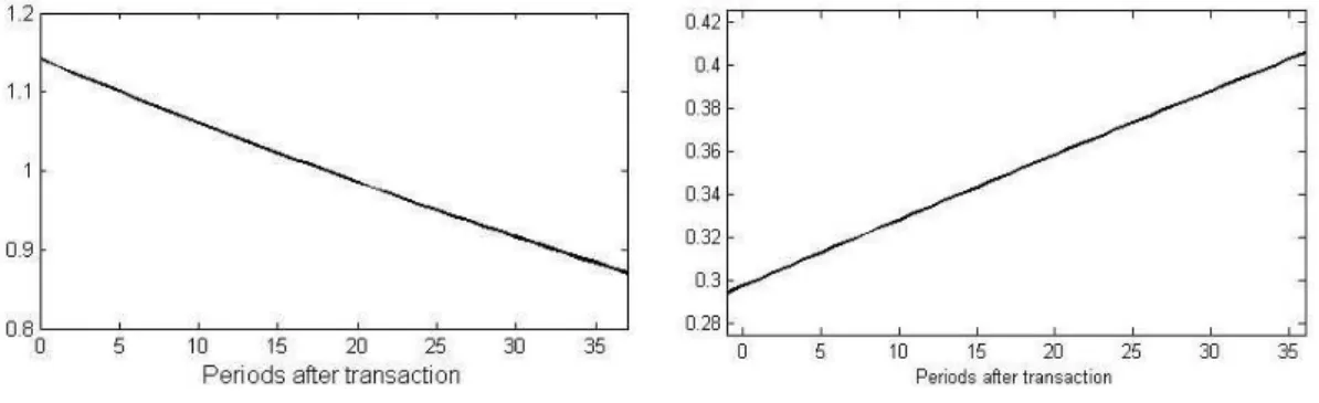
In Figure 2 and 3 we see the steady state behavior of consumption and labor supply during a holding period. We see that consumption of the households will be decreasing during the holding period. This happens for two reasons. Because the opportunity cost of consumption at the end of the holding period is higher than the opportunity cost of consumption at the beginning of the holding period. This cost is higher at the end of the holding period because the agents need to safe the money at the bank account during more periods, which, in the case of a positive in‡ation rate, reduces the real value of the money. On the other hand, due to the intertemporal discount rate agents prefer consumption today instead of consumption later. We can see this in equation (19)
from the marginal rate of substitution between leisure and consumption, (20) and (21), we know that when consumption is lower, labor supply will be higher. So once consumption is decreasing during the holding period, labor supply will be increasing. In the second place, the marginal revenue of one hour work is higher in the beginning and lower at the end of each holding period.
Figure 2: Consumption Figure 3: Labor Supply
4
Monetary Policy Shock
As mentioned before I will identify the monetary policy shock as an exogenous shock to the nominal interest rate. I assume that the deviation of the nominal interest rate of his steady state value follows a AR(1) process: R~t = R~t 1 +"t, where I
…x = 0:87, "0 = 0:01 and "t = 0, for t = 1;2; :::, as in Alvarez et al (2009). I
assume that the agents of the model do not anticipated the shock and only observe it at the beginning oft = 0. After the shock I assume that their does not exist any uncertainty to be able to isolate the e¤ects of the interest rate shock.
However, at the moment of the shock, t = 0, to fully describe the monetary policy one needs to impose some initial condition about the price level or about the nominal money supply. I will assume that the government controls the nominal money supply at t = 0. More, I assume that the nominal money supply, at t = 0, continues to grow at its steady state rate. In practical terms, this is equivalent to assuming, as in Alvarez et al (2009), that the shock to the nominal interest rate does not a¤ect the price level att= 0.
4.1
Solution Method
Unlike Alvarez et al (2009), I will solve the equilibrium response of the economy of the model in a simple non-linear way. I start to assume that the economy, after the interest rate shock, will be back to its initial steady state after a su¢ciently high number of periods, t . This way I can solve the response of in‡ation, output, consumption and labor supply backwards. I will start to solve the response for
t=t 1, then for t=t 2and so on. Note that the path of the nominal interest rate, fRtg1t=0, is exogenous and therefore known.
So, the economy will be back to its initial steady state at t = t . This means that in‡ation, output, consumption and labor supply will be back to their initial steady state values
t =
Yt = Y
Now I will obtain in‡ation, output, consumption and hours of labor fort =t 1. This way I have2N+2unknowns and will also need2N+2equations. The equations will be the following:
-N 1intra-holding optimal conditions for consumption betweent=t 1and
t=t
u0[ct 1(s 1)] = t
u0[ct (s)],
for s = 1;2; :::; N 1
-1inter-holding optimal condition for consumption betweent=t 1andt=t u0[ct 1(N 1)] =
t
u0[ct (0)]Rt NRt N+1:::Rt 1
-N marginal rate of substitution conditions between leisure and consumption at
t=t 1
u0[ht(s)] u0
[ct(s)]
= A + 1
Rt 1 s:::Rt 1
(1 )
for s = 0;1; :::; N 2
u0[ht(N 1)] u0
[ct(N 1)]
=A 1
Rt N:::Rt 1
- 1market clearing condition for the labor market att =t 1 1
N NX1
s=0
ht 1(s) =Lt 1
- and 1market clearing condition for the good market at t=t 1 1
N NX1
s=0
ct 1(s) =Yt 1
By solving this nonlinear system of2N+ 2 equations and unknowns I obtain t 1, Yt 1, fct 1(s)gsN=01 and fht 1(s)gNs=01.7
Once I know the values of the main variables for t =t 1, I can use the same method to obtain in‡ation, output, consumption and hours of labor fort =t 2. Using the same equations as above, but now fort=t 2, I have again a system of
2N+ 2equations and unknowns. By repeating this method I obtain the response of the main variables of the model to the interest rate shock fort =N 1; N; :::; t 1; t . To obtain the response of the economy for the …rstN 1periods the equations used change a little. The reason therefore is that for the …rst N 1 periods at least one of the types of households will be in their …rst holding period and, hence, the inter-holding optimal conditions and the marginal rate of substitution between leisure and consumption will depend on the ratio of the Lagrange multipliers, as we can see in (12), (14) and (15). This way, for the …rst N 1 periods, I have N 1
additional unknowns, n (s)oN 1
s=0 , and therefore will also need N 1 additional
right solution.8 So, this way I will add the following N 1 equations
N 1
X
t=s
Pt sct s(t) = M0(s) + N 2
X
t=s
Wt sht s(t),
for s = 1;2; :::; N 1
These equations contain consumption and labor supply until the …rst transaction is made, therefore, for the …rst N 1 periods I solve the response of the economy as one only system. This way, the system will contain(N 1) (2N + 2) + (N 1)
unknowns: t; Yt;fct(s)gNs=01 and fht(s)gsN=01 for t = 0;1; :::N 2 and
n
(s)oN 1 s=0 .
The equations of the system will be the following: for t= 0;1; :::; N 2;
- N 1 intra-holding optimal conditions for consumption betweent and t+ 1
u0[ct(s 1)] = t+1
u0[ct+1(s)],
for s = 1;2; :::; N 1
- 1inter-holding optimal condition for consumption between t and t+ 1
u0[ct(N 1)] = t+1
u0[ct+1(0)] 1 +
(s) 1
Qt+1
-N marginal rate of substitution conditions between leisure and consumption at
t
- if the household has already made a transaction at t
8To do this I use the optimal conditions for the …rst holding period and the fact that if
Zt(N 1) > 0, for t = 0;1; :::; N 2, then the bank account constraint for the …rst holding
u0[ht(s)] u0
[ct(s)]
= A + 1
Rt 1 s:::Rt 1
(1 )
for s = 0;1; :::; N 2
- if the household has not made yet a transaction at t u0[ht(s)]
u0
[ct(s)]
= A Qt+N s+ (1 )Qt+1+ (s)
Qt+N s+ (s)
for s = 0;1; :::; N 2
u0[h
t(N 1)] u0[c
t(N 1)]
=A Qt+1 Qt+1+ (s)
- 1market clearing condition for the labor market att
1
N NX1
s=0
ht 1(s) =Lt 1
- 1market clearing condition for the good market at t
1
N NX1
s=0
ct 1(s) =Yt 1
- and N 1bank account constraints
T1(s) 1
X
t=0
Ptct(s) =M0(s) + T1(s) 2
X
t=0
Wtht(s)
So, solving this system of (2N + 2) (N 1) + (N 1) equations and unknowns I obtain t; Yt;fct(s)gsN=01 and fht(s)g
N 1
s=0 for t= 0;1; :::N 2.9
9Note that for the bank account constraints I need to use the assumption that the nominal
money supply grows at its steady state rate att= 0. In practice, I assume that the in‡ation rate
4.2
Results
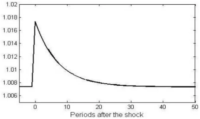
The main goal of this dissertation is to analyze the robustness of the results obtained by Alvarez et al (2009). They obtain the response of in‡ation in a model very similar to the one presented here. The main di¤erence between their model and my model is that in their model output is exogenous and constant, while in my model output is endogenous and responds to the interest rate shock. To be able to obtain the results of an endowment economy I will …x the elasticity of labor, , very close to zero. This way labor supply will be constant and will not respond to the interest rate shock. By doing this I replicate the results of Alvarez et al (2009). Next, to be able to analyze the di¤erence between the two types of models I increase and, consequently, labor supply will respond to the shock and output will be endogenous. Figure 4 shows the exogenous shock to the nominal interest rate. As mentioned before, at t = 0 the interest rate increases with 100 basis point and returns then slowly back to his initial steady state value.
Figure 4: Gross Nominal Interest Rate
elasticity of labor until = 1;75, which is the benchmark case; in which the agents spent around 35 per cent of their time working. As we can see, output starts to respond to the shock. At the moment of the shock output rises, until at most0:65
per cent above its steady state value, but then starts to decrease and around three months after the shock output is below its steady state value. Then after around one year output starts to recover and goes slowly back to its steady state.
Figure 5: Output - = 0 Figure 6: Output - = 0:1
Figure 9: Output - = 1 Figure 10: Output - = 1:75
Figure 11: In‡ation - = 0 Figure 12: In‡ation - = 0:1
Figure 13: In‡ation - = 0:25 Figure 14: In‡ation - = 0:5
Figure 15: In‡ation - = 1 Figure 16: In‡ation - = 1:75
It is important to point out that when I increase the elasticity of labor the annual average velocity of money changes. As in Alvarez et al (2009) I set N = 38 and
the velocity of money increases until around 1:65. To be able to obtain an average velocity of money equal to1:5I need to increase the number of periods between two …nancial transactions, N, or to decrease the part of the payment received on the bank account; . For example, if I increaseN from38to42in the case of = 1:75, the annual average velocity of money will decrease from 1:65 to 1:5. The results presented here are robust to this changes.
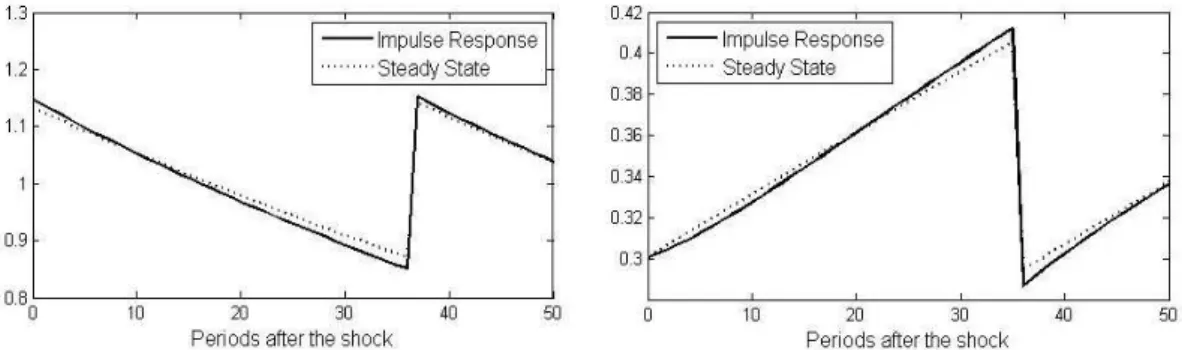
Now I will take a closer look at the response of output and in‡ation in case of a labor elasticity equal to1:75. Below I show the behavior of three types of households after the interest rate shock: a household which makes a transaction at the moment of the shock, type s = 0 at t = 0; a household which will make a transaction 18
periods after the shock, type s = 18 at t = 0; and a household which has made a transaction the period before the shock and now only will make a transaction after
37 periods, type s = 1 at t = 0. By showing these three types of household I will try to understand what the behavior of the di¤erent types of households is.
As we can see, the household which makes a transaction at t= 0 (types = 0 at
the opposite. This is a consequence of the wealth e¤ect resulting from the higher interest rate. When this e¤ect starts to dominate, which will be after some months, output will come below its initial steady state value and the economy will get in a recession.
Figure 17: Consumption of a Household of types = 0 att = 0
Figure 18: Labor Supply of a Household of type s= 0 att= 0
Figure 19: Consumption of a Household of type s= 18 at t= 0
Figure 21: Consumption of a Household of type s= 1 att= 0
Figure 22: Labor Supply of a Household of type s= 1 at t= 0
5
Conclusion
With this dissertation I try to contribute to the literature about monetary policy shocks in general equilibrium models with market segmentation. I use a very similar model to the one used by Alvarez et al (2009), but in my model production is endo-genous. I introduce an exogenous shock to the nominal interest rate and calculate the response of the main variables of the model.
shock there exist a positive e¤ect on output but after a few months the economy gets into a recession and will slowly return to its steady state.
Further, in this dissertation I introduce a di¤erent and simple nonlinear way to solve the response of the model to the interest rate shock. By assuming that the economy will be back at its initial steady state at a su¢ciently hight , I am able to solve the equilibrium response of the model backwards.
The following steps in this research should be in two directions. In the …rst place, one should introduce the market segmentation into the optimization process of the agents. This way the agents are able to adjust the number of periods between two …nancial transactions after the interest rate shock. It is important to analyze in which way turning the market segmentation endogenous changes the results ob-tained in this dissertation. A good example of how to introduce endogenous market segmentation into this type of models is Silva (2012). However, this lies behind the goals of this dissertation.
A
Appendix
First I will substitute the cash-in-advance constraints for each holding period, (7) and (8), into the intertemporal budget constraint, (1), and obtain
1
X
t6=Tj(s)
QtMt(s) +
1
X
j=0 QTj(s)
Tj+1(s) 1
X
t=Tj(s)
Ptct(s) +ZT1(s) 1
1
X
j=0 QTj(s)
Tj+1(s) 2
X
t=Tj(s)
Wtht(s)
0(s) +
1
X
t=0
Qt+1Wtht(s) +
1
X
t=0
Qt+1Zt(s)
1
X
t=0
Qt+1 t
Now I will substitute the bank account constraint for t6=Tj(s), (2), into the
equa-tions above and obtain
1
X
t6=Tj(s)
Qt Wt 1ht 1(s) +
1
X
t6=Tj(s)
QtZt 1(s) +
1
X
j=0 QTj(s)
Tj+1(s) 1
X
t=Tj(s)
Ptct(s)
+ZT1(s) 1
1
X
j=0 QTj(s)
Tj+1(s) 2
X
t=Tj(s)
Wtht(s)
0(s) +
1
X
t=0
Qt+1Wtht(s) +
1
X
t=0
Qt+1Zt(s)
1
X
t=0
Qt+1 t
1
X
j=0 QTj(s)
Tj+1(s) 1
X
t=Tj(s)
Ptct(s) 0(s) + T1(s) 2
X
t=0
Wtht(s) +
+
1
X
j=1 QTj(s)
Tj+1(s) 2
X
t=Tj(s) 1
Wtht(s) + (1 )
1
X
t=0
Qt+1Wtht(s) +
+
1
X
j=1
QTj(s)ZTj(s) 1(s) ZT1(s) 1 1
X
t=0
Qt+1 t
Now knowing thatZTj(s) 1 = 0 for j = 2;3; ::: I obtain 1
X
j=0 QTj(s)
Tj+1(s) 1
X
t=Tj(s)
0(s) + QT1(s) 1 ZT1(s) 1(s) +
+ T1(s) 2
X
t=0
Wtht(s) +
1
X
j=1 QTj(s)
Tj+1(s) 2
X
t=Tj(s) 1
Wtht(s) +
+
1
X
t=0
Qt+1(1 )Wtht(s)
1
X
t=0
References
Alvarez, F., Atkeson, A. & Kehoe, P. (2002). Money, Interest Rates, and Exchange Ratess with Endogenously Segmented Markets. Journal of Political Economy 110 (1), 73-112.
Alvarez, F., Atkeson, A. & Edmond, C. (2009). Sluggish Responses of Prices and In‡ation to Monetary Shocks in an Inventory Model of Money Demand.Quarterly Journal of Economics 124 (3), 911-967.
Baumol, W. (1952). The Transaction Demand For Cash: An Inventory Theoretic Approach. The Quarterly Journal of Economics 66 (4), 545-556.
Grossman, S. & Weiss, L. (1983). A Transactions-Based Model of the Monetary Transmission Mechanism. The American Economic Review 73 (5), 871-880. King, R., Plosser, C. & Rebelo, S. (1987). Production, Growth and Business Cycles.
Journal of Monetary Economics 21, 195-232.
Rotemberg, J. (1984). A Monetary Equilibrium Model With Transactions Costs.
Journal of Political Economy 92 (1), 40-58.
Silva, A. (2012). Rebalancing Frequency and the Welfare Cost of In‡ation.American Economic Journal: Macroeconomics 4 (2), 153-183.
Tobin, J. (1956). The Interest-Elasticity of Transactions Demand For Cash. The Review of Economics and Statistics 38 (3), 241-247.