Two-dimensional body of maximum mean
resistance
Paulo D. F. Gouveia
a,∗
Alexander Plakhov
b,cDelfim F. M. Torres
baBragan¸ca Polytechnic Institute, 5301-854 Bragan¸ca, Portugal
bUniversity of Aveiro, 3810-193 Aveiro, Portugal
cAberystwyth University, SY23 3BZ Aberystwyth, UK
Abstract
A two-dimensional body, exhibiting a slight rotational movement, moves in a rarefied medium of particles which collide with it in a perfectly elastic way. In previously realized investigations by the first two authors, Plakhov & Gouveia (2007, Non-linearity, 20), shapes of nonconvex bodies were sought which would maximize the braking force of the medium on their movement. Giving continuity to this study, new investigations have been undertaken which culminate in an outcome which represents a large qualitative advance relative to that which was achieved earlier. This result, now presented, consists of a two-dimensional shape which confers on the body a resistance which is very close to its theoretical supremum value. But its interest does not lie solely in the maximization of Newtonian resistance; on re-garding its characteristics, other areas of application are seen to begin to appear which are thought to be capable of having great utility. The optimal shape which has been encountered resulted from numerical studies, thus it is the object of ad-ditional study of an analytical nature, where it proves some important properties which explain in great part its effectiveness.
Key words: body of maximal resistance, billiards, Newton’s aerodynamic problem, retroreflector
2000 MSC: 74F10, 65D15, 70E15, 49K30, 49Q10
∗ Corresponding author.
Email addresses: [email protected] (Paulo D. F. Gouveia),[email protected]
1 Introdution
One area of investigation in contemporary mathematics is concerned with the search for shapes of bodies, within predefined classes, which permit the minimization or maximization of the resistance to which they are subjected when they move in rarefied media. The first problem of this nature goes back to the decade of the 1680s, a time when Isaac Newton studied a problem of minimum resistance for a specific class of convex bodies, which moved in media of infinitesimal particles, rarefied to such a degree that it was possible to discount any interaction between the particles, and in which the interaction of these with the bodies could be described as perfectly elastic collisions [1]. More recently we have witnessed important developments in this area with the broadening of study to new classes of bodies and to media with characteristics which are less restrictive: problems of resistance in non-symmetrical bodies [2– 6], in nonconvex bodies of single collisions [7,4,8,9] and multiple collisions [10– 12], bodies of developable surfaces [9], considering collisions with friction [13] and in media with positive temperature [14]. However most studies which have been published have given special attention to classes of convex bodies.
The convexity of a body is a sufficient condition for the resistance to be solely a function of singular collisions — all the particles collide at once with the body. This attribute allows us to considerably reduce the complexity of the problems dealt with. Even the various studies of classes of nonconvex bodies which have emerged, especially in the last decade, are based almost always on conditions that guarantee a single impact per particle — [7,4,8,9]. Only very recently have there begun to emerge some studies supposing multiple reflections (see, e.g. [10–12]).
In the class of convex bodies, the problem is normally reduced to the mini-mization of Newton’s functional — an analytical formula for the value of the resistance. But, in the context of nonconvex bodies, there is not any simple formula known for the calculation of the resistance. Even if it is extremely complex, in general, to deal analytically with problems of multiple collisions, for some specific problems of minimization the job has not been revealed to be particularly difficult, there even being some results already available [10,11]. If, on the other hand, we consider the problem of maximization, then in this case the solution becomes trivial — for any dimension, it is enough that the front part of the body is orthogonal to the direction of the movement.
the device rotates slowly around itself.
The problem of resistance minimization for rotating nonconvex two-dimensional bodies has already been studied in [12,15]: it was shown that the maximal re-duction of resistance, as compared with the convex case, is approximately 1.22%. In its turn, the problem of maximization of the average resistance of bodies in rotation is far from being trivial, in contrast with that which occurs when we deal with purely translational movement. This class of problems was, therefore, the object of study of the work carried out by the authors in [16,17]: nonconvex shapes of bodies were investigated which would maximize the re-sistance that they would have to confront if they moved in rarefied media, and, simultaneously, exhibited a slight rotational movement. With the numer-ical study which was executed, various geometrnumer-ical shapes were found which conferred on the bodies rather interesting values of resistance: but it was in later investigations, performed in the follow-up of this work, that the authors managed to arrive at the best of the results — a two-dimensional shape which confers on the body a resistance very near to its maximum theoretical limit. It is this latest result which now is presented here.
The presentation of the work is organized in the following way. In section 2, we begin by defining, for the two-dimensional case, the problem of maximization, which is the object of the present study. Then, in section 3, we describe the nu-merical study which was realized in the tracking of the body of maximum resis-tance and we present the main original result of this study: a two-dimensional shape which maximizes Newtonian resistance. The two-dimensional shape is then the object of study in section 4, where some important properties are shown which help to explain the value of resistance which it displays. In sec-tion 5, we present the main conclusions of our study and include some notes on possible working directions to undertake in the future. Finally, in appendices A and B, proofs of theorems 1 and 2 are provided.
2 Definition of the problem for the two-dimensional case
Consider a disc in slow and uniform rotation, moving in a direction parallel to its plane. We will designate the disc of radius r by Cr and its boundary
by ∂Cr. We then remove small pieces of the disc along its perimeter, in an
ε-neighborhood of ∂Cr, withε ∈R+ of value arbitrarily small when compared
with the value of r. We are thus left with a new body B defined by a subset of Cr and characterized by a certain roughness along all its perimeter. The
circular contour, in this case), that is, learning the normalized value
R(B) = Resistance(B) Resistance(Cr)
. (1)
It is possible, from the beginning, to know some important reference values for the normalized resistance:R(Cr) = 1 and the value of the resistanceR(B)
will have to be found between 0.9878 ([12,15]) and 1.5. The value 1.5 will be hypothetically achieved if all the particles are reflected by the body with the velocity v+ (velocity with which the particles separate definitively from the body) opposite to the velocity of incidencev(velocity with which the particles strike the body for the first time),v+ =−v, the situation in which the
maxi-mum momentum is transmitted to the body. It is also possible for us to know the resistance value of some elementary bodies of the typeB. This is the case, for example, of discs with the contour entirely formed by rectangular inden-tations which are arbitrarily small or with the shape of rectangular isosceles triangles. As was proved in [17], these bodies are associated with resistances, respectively, of R= 1.25 andR =√2.
Apart from being defined in the disc Cr, it is assumed that the body to be
maximized is a connected set B ∈ R2, with piecewise smooth boundary ∂B.
Therefore, let us consider a billiard inR2\B. An infinitesimal particle moves
freely, until, upon colliding with the bodyB, it suffers various reflections (one at least) at regular points of its boundary ∂B, ending up by resuming free movement which separates it definitively from the body. Denote by convB the convex hull ofB. The particle intercepts the∂(convB) contour twice: when it enters into the set convB and in the moment that it leaves. L =|∂(convB)| is considered the total length of the curve ∂(convB), and the velocity of the particle is in the first and second moments of interception represented by v
and v+, and x and x+ the respective points where they occur. As well, the
angles which the vectors−vandv+make with the outer normal vector to the section of ∂(convB) between the points x and x+ are designated ϕ and ϕ+.
They will be positive if they are defined in the anti-clockwise direction from the normal vector, and negative in the opposite case. With these directions, bothϕ as well asϕ+ take values in the interval [−π/2, π/2].
Representing the cavities which characterize the contour of B by subsets Ω1,Ω2, . . ., which in their total make up the set convB \B, the normalized
resistance of the body B (equation (1)) takes the following form (cf. [17]):
R(B) = |∂(convB)| |∂Cr|
L0
L +
X
i6=0
Li
LR( ˜Ωi)
, (2)
being L0 =|∂(convB)∩∂B|the length of the convex part of the contour∂B,
Li =|∂(convB)∩Ωi|, withi= 1,2, . . ., the size of the opening of the cavity Ωi,
segment of unitary size, with
R( ˜Ωi) =
3 8
Z 1/2
−1/2
Z π/2
−π/2
1 + cosϕ+(x, ϕ)−ϕcosϕdϕdx. (3)
The function ϕ+ should be seen as the angle of departure of a particle which
interacts with a cavity ˜Ωi that has opening of unit size and is similar to Ωi,
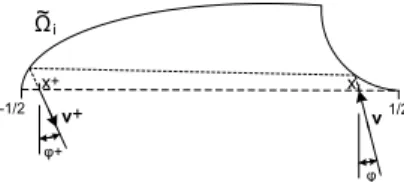
with the similarity factor 1/Li — see illustration of figure 1.
1/2
φ 1/2
x
+
φ+
x+ i
~
Fig. 1. Example of trajectory of a particle which interacts with a cavity ˜Ωi.
From equation (2), we understand that the resistance of B can be seen as a weighted mean (PiLi/L= 1) of the resistances of the individual cavities which
characterize all its boundary (including resistance of the convex part of the boundary), multiplied by a factor which relates the perimeters of the bodies convB and Cr. Thus, maximizing the resistance of the B body amounts to
maximizing the perimeter of convB (|∂(convB)| ≤ |∂Cr|) and the individual
resistances of the cavities Ωi.
Having found the optimal shape Ω∗, which maximizes the functional (3), the
body of maximum resistanceB will be that whose boundary is formed only by the concatenation of small cavities with this shape. We can therefore restrict our problem to the sub-class of bodiesB which have their boundary integrally covered with equal cavities, and in doing so admit, without any loss of gener-ality, that each cavity Ωi occupies the place of a circle arc of size ε ≪ r. As
with Li = 2rsin(ε/2r), the ratio between the perimeters takes the value
|∂(convB)| |∂Cr|
= sin(ε/2r)
ε/2r ≈1−
(ε/r)2
24 , (4)
or that is, given a body B of a boundary formed by cavities similar to Ω, from (2) and (4), we conclude that the total resistance of the body will be equal to the resistance of the individual cavity Ω, less a small fraction of this value, which can be neglected whenε ≪r,
R(B)≈R(Ω)− (ε/r)
2
24 R(Ω). (5)
Thus, our research has as its objective the finding of cavity shapes Ω which maximize the value of the functional (3), whose limit we know to be found in the interval
as is easily proven using (3): if Ω is a smooth segment, ϕ+(x, ϕ) = −ϕ and
R(Ω) = 38 R−1/21/2R−π/2π/2(1 + cos (2ϕ)) cosϕdϕdx= 1; in the conditions of maxi-mum resistanceϕ+(x, ϕ) =ϕ, thusR(Ω) ≤ 3
8 R1/2
−1/2
Rπ/2
−π/22 cosϕdϕdx= 1.5.
3 Numerical study of the problem
In the class of problems which we are studying, only for some shapes of Ω which are very elementary is it possible to derive an analytical formula of their re-sistance (3), as we saw in the rectangular and triangular shapes previously referred to. For somewhat more elaborate shapes, the analytical calculation becomes rapidly too complex, if not impossible, given the great difficulty in knowing the function ϕ+ : [−1/2,1/2]×[−π/2, π/2] → [−π/2, π/2], which
as we know, is intimately related to the format of the cavity Ω. Therefore, recourse to numerical computation emerges as the natural and inevitable ap-proach in order to be able to investigate this class of problems.
There have been developed various computational models which simulate the dynamics of billiard in the cavity. The algorithms of construction of these models, as well as the those responsible for the numerical calculation of the associated resistance, were implemented using the programming language C, given the computational effort involved (language C was created in 1972 by Dennis Ritchie; for its study we suggest, among the extensive documentation available, that which is the reference book of its language, written by Brian Kernighan and Dennis Ritchie himself, [18]). The efficiency of the object code, generated by the compilers of C, allowed the numerical approximation of (3) to be made with a sufficiently elevated number of subdivisions of the intervals of integration — between some hundreds and various thousands (up to 5000). The results were, because of this, obtained with a precision which reached in some cases 10−6. This precision was controlled by observation of the difference
between successive approximations of the resistance R which were obtained with the augmentation of the number of subdivisions.
For the maximization for the resistance of the idealized models, there were used the global algorithms of optimization of the toolbox “Genetic Algorithm and Direct Search” (version 2.0.1 (R2006a), documented in [19]), a collection of functions which extends the optimization capacities of the MATLAB numer-ical computation system. The option for Genetic and Direct search methods is essentially owed to the fact that these do not require any information about the gradient of the objective function nor about derivatives of a higher order — as the analytical form of the resistance function is in general unknown (given that it depends onϕ+(x, ϕ)), this type of information, if it were
would greatly impede the optimization process. The MATLAB computation system (version 7.2 (R2006a)) was also chosen because it had functionalities which allowed it to be used for the objective function the subroutine compiled in C of resistance calculation, as well as theϕ+(x, ϕ) function invoked in itself.
3.1 “Double Parabola”: a two-dimensional shape which maximizes resistance
In the numerical study which the authors carried out in [16,17], shapes of Ωf defined by continuous and piecewise differentiable f : [−1/2,1/2] → R+
functions were sought for:
Ωf ={(x, y) : −1/2≤x≤1/2, 0≤y≤f(x)}, (7)
with the interval [−1/2,1/2]× {0} being the opening.
The search for the maximum resistance was begun in the class of continuous functionsf with derivativef′piecewise constant, broadening later to the study
of classes of functions with the second derivativef′′ piecewise constant. In the
first of the cases the contour of Ωf is a polygonal line, and in the second, a
curve composed of parabolic arcs. Not having been able with these shapes to exceed the value of resistanceR = 1.44772, we decided, in this new study, to extend the search to shapes different from those considered in (7). We studied shapes Ωg defined by functionsx of y of the following form:
Ωg ={(x, y) : 0≤y ≤h, −g(y)≤x≤g(y)}, (8)
whereh >0 andg : [0, h]→R+
0 is a continuous function withg(0) = 1/2 and
g(h) = 0.
The new problem of maximum resistance studied by us can therefore be for-mulated in the following way:
To find supgR(Ωg) in the continuous and piecewise differentiable functions
g : [0, h]→R+0, such as g(0) = 1/2 and g(h) = 0, with h >0.
Similarly to the study which was carried out for the sets Ωf, in the search
for shapes Ωg, the functions g were considered piecewise linear and piecewise
quadratic. If in the classes of linear functions it was not possible to achieve a gain in resistance relative to the results obtained for the sets Ωf, in the
quadratic functions the results exceeded the highest expectations: there was found a shape of cavity Ωg which presented the resistanceR = 1.4965, a value
follows the description of the best result which was obtained, encountered in the class of quadratic functions x=±g(y).
The value of resistance of the sets Ωg were studied, just as defined in (8), in
the class of quadratic functions
gh,β(y) =αy2+βy+ 1/2, for 0≤y≤h ,
where h > 0 and α = −βhh−21/2 (given that gh,β(h) = 0). In the optimization of the curve, the two parameters of the configuration were made to vary: h, the height of the ∂Ωg curve, and β, in its slope at the origin (g′(0)). In this
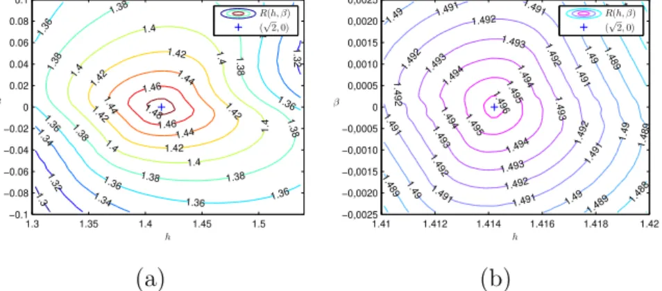
class of functions the algorithms of optimization converge rapidly towards a very interesting result: the maximum resistance was reached with h= 1.4142 and β = 0.0000, and assumed the value R = 1.4965, that is, a value 49.65% above the resistance of the rectilinear segment. This result seems to us really interesting:
(1) it represents a considerable gain in the value of the resistance, relative to the best result obtained earlier (in [16,17]), which was situated 44.77% above the reference value;
(2) The corresponding set Ωg has a much more simple shape than that of set
Ωf associated with the best earlier result, since it is formed by two arcs
of symmetrical parabolas, while the earlier one was made up of fourteen of these arcs;
(3) this new resistance value is very near to its maximal theoretical limit, which, as is known, is found 50% above the value of reference;
(4) The optimal parameters appear to assume value which give to the set Ωg
a configuration with very special characteristics, as in what follows will be understood.
Note that the optimal parameters appear to approximate the valuesh=√2 = 1.41421. . . and β = 0. The following question can therefore be put:
Are these not the exact values of the optimal parameters?
The graphical representation of the function R(h, β) through the level curves, figure 2, are effectively in concordance with this possibility — note that the level curves appear perfectly centered on the (√2,0) coordinates; marked on the figure by “+” . Note also, in figure 3, the resistance graphR(h) forβ = 0, where it can equally be perceived that there is a surprising elevation of resis-tance when h → √2. Thus the resistance of the Ωghβ cavity was numerically
calculated with the exact values h = √2 and β = 0, the result having con-firmed the value 1.49650.
1.3 1.32 1.32 1.34 1.34 1.34 1.36 1.36 1.36 1.36 1.36 1.36 1.36 1.38 1.38 1.38 1.38 1.38 1.38 1.38 1.4 1.4 1.4 1.4 1.4 1.4 1.42 1.42 1.42 1.42 1.42 1.44 1.44 1.44 1.46 1.46 1.48 h β
1.3 1.35 1.4 1.45 1.5
−0.1 −0.08 −0.06 −0.04 −0.02 0 0.02 0.04 0.06 0.08 0.1
R(h, β) (√2,0)
1.487 1.488 1.488 1.489 1.489 1.489 1.489 1.49 1.49 1.49 1.49 1.49 1.491 1.491 1.491 1.491 1.491 1.491 1.491 1.492 1.492 1.492 1.492 1.492 1.492 1.492 1.493 1.493 1.493 1.493 1.493 1.494 1.494 1.494 1.494 1.495 1.495 1.496 h β
1.41 1.412 1.414 1.416 1.418 1.42
−0,0025 −0,0020 −0,0015 −0,0010 −0,0005 0 0,0005 0,0010 0,0015 0,0020 0,0025
R(h, β) (√2,0)
(a) (b)
Fig. 2. Level curves of theR(h, β) function.
0 1 2 3 4
1 1.1 1.2 1.3 1.4 1.5 h R(h)
√ 2→
Fig. 3. Resistance graphicR(h) for β = 0.
a particular case with which is associated special characteristics which could justify the elevated value of resistance presented. The two sections of the shape are similar arcs of two parabolas with the common horizontal axis and concavities turned one towards the other — see figure 4. But the particularity of the configuration resides in the fact that the axis of the parabolas coincides with the line of entry of the cavity (axis ofx), and that the focus of each one coincides with the vertex of the other.
1.25 1.0 0.0 0.5 0.25 −0.25 0.75 0.25 0.5 0.0 −0.5 (a) (b)
Fig. 4. (almost) Optimal 2D shape — theDouble Parabola.
only a few small irregularities for ϕ angles of little amplitude. Noting this characteristic, and taking into account that the integrand function almost does not depend on x, the resistance was calculated, for this shape in particular, using the rule of Simpson 1/3 in the integration in order to ϕ. The double integration in the equation (3) was thus numerically approximated by the following expression:
R= 1
2∆x∆ϕ
Nx
X
i=Nx/2+1
Nϕ−1
X
k=1
wk
1 + cosϕ+(x
i, ϕk)−ϕk
cosϕk, (9)
with wk = 2 for k odd and wk = 1 for k even, xi = −1/2 + (i−1/2)∆x,
∆x= 1/Nx,ϕk=−π/2+k∆ϕand ∆ϕ =π/Nϕ.Nx andNϕare the number of
sub-intervals to consider in the integration of the variablesxandϕ(both even numbers), respectively, and ∆x and ∆ϕ the increments for the correspondent discreet variables. Given that the shape Ωg√
2,0 presents horizontal symmetry,
the first summation of the expression considers only the second half of the interval of integration of the variable x.
In order to be easily referred to, this shape of cavity (figure 4a) will be, from here on, named simply “Double Parabola”. Thus, in the context of this paper, the term “Double Parabola” should be always understood as the name of the cavity whose shape is described by two parabolas which, apart from being geometrically equal, find themselves “nested” in the particular position to which we have referred.
Since the resistance of the Double Parabola assumes a value which is very close to its theoretical limit, in a final attempt to achieve this limit, it was resolved to extend the study even further to other classes of functionsg(y) which admit the Double Parabola as a particular case or which allow proximate configurations of this nearly optimal shape. In all these cases the best results were invariably obtained when the shape of the curves approximated the shape of the Double Parabola, without ever having overtaken the value R= 1.4965. It was begun by considering functions g(y) piecewise quadratic, including curves splines, without achieving interesting results; only for functionsg(y) of 2 or 3 segments was it possible to approximate the resistance and the shape of the Double Parabola. Cubic and bi-quadratic functions g(y) were also considered1, but
in both cases the process of optimization brought them proximate to the curves of quadratic order, with the coefficients of greater order taking values which were almost zero. The problem was studied in the class of conical sections,
1 In the bi-quadratic curves, the point of interception of the trajectory of the
considering, for lateral facets of the cavity, two symmetrical arcs either of an ellipse or of a hyperbole. Also in these cases the arcs assumed a shape very close to the arcs of the parabolas.
The Double Parabola being the best shape encountered, and dealing with a nearly optimal shape, in the section which follows it is the object of deeper study, of an essentially analytical nature, where the reasons for its good per-formance are sought.
4 Characterization of the reflections in the shape “Double Parabola”
Each one of the illustrations of figure 5 shows, for the “Double Parabola”, a concrete trajectory, obtained with our computational model. It is comforting
(a) x= 0.45, ϕ= 75◦. (b) x= 0.45, ϕ = 55◦. (c) x= 0.45, ϕ= 35◦.
(d) x= 0.3,ϕ = 75◦. (e) x= 0.0, ϕ= 35◦. (f) x= 0.48, ϕ= 5◦.
Fig. 5. Example of trajectories obtained with the computational model.
to verify that, with the exception of one trajectory, in all the others the par-ticle emerges from the cavity with a velocity which is nearly opposite to that which was its entry velocity. This is the “symptom” which unequivocally char-acterizes a cavity of optimal performance. Even in the case of the trajectory of the illustration (f), the direction of the exit velocity appears not to vary greatly from that of entry.
essentially empirical, the results of the study which follow are heading in the direction of confirming that one very significant part of the “benign” trajec-tories — those in which the vectors velocity of entry and of exit are nearly parallel; we call them so because they represent positive contributions to the maximization of resistance — suppose exactly three reflections.
We now will try to interpret another type of results obtained with our compu-tational model, commencing with the graphical representation of the distribu-tion of the pairs (ϕ, ϕ+) on the Cartesian plane — see figure 6. This graph was
produced with 10.000 pairs of values (x, ϕ), generated by a random process of uniform distribution.
−80 −60 −40 −20 0 20 40 60 80
−80 −60 −40 −20 0 20 40 60 80
ϕ ϕ+
−ϕ0→ ←ϕ0
Fig. 6. Distribution of the (ϕ, ϕ+) pairs on the Cartesian plane.
The points concentrate themselves on the proximities of the diagonalϕ=ϕ+,
which revealing of good behavior on the part of the cavity. In addition, with these results it is shown that the response of the cavity deteriorates as ϕ
approaches zero. Therefore, it begins to be understood that the “benign” trajectories have their origin essentially in entry angles of elevated amplitude.
If we consider figure 6, there appears to exist an additional perturbation in the behavior of the cavity when the amplitude of the entry angle is inferior to about 20◦, which means that some (ϕ, ϕ+) pairs become, in relation to the
others, more dispersed and more distant from the diagonalϕ+ =ϕ. We have
already called attention to the possible importance of the three reflections in the degree of approximation verified in the angles ϕ and ϕ+. It occurs to
us, therefore, to put the following question: is it not precisely the number of reflections that, on differentiating themselves from the 3 occurrences, interfere so negatively with the behavior of the cavity? The investigations that follow will demonstrate, among other things, that our suspicion on this point has a basis.
The following theorem says that for ϕ outside some interval (−ϕ0, ϕ0), the
number of reflections is always three. The proof is presented in appendix A.
Theorem 1 Forϕentry angles superior (in absolute value) toϕ0 = arctan √
2 4
19.47◦, the number of reflections to which the particle is subjected in the
in-terior of the Double Parabola cavity is always equal to three, and they occur alternately on the left and right faces of the cavity, no matter what the entry position may be.
As a way to verify that the deductions which we have made are effectively in concordance with the numerical results of the computational model which was developed, we present one more graph, figure 7, produced with 10.000 pairs of (x, ϕ) values, generated randomly with uniform distribution. As can be
ob-−80 −60 −40 −20 0 20 40 60 80
0 1 2 3 4 5 6 7 8 9
ϕ
n
◦
o
f
re
fl
ec
ti
o
n
s
−ϕ0→ ←ϕ0
Fig. 7. Distribution of the (ϕ, nr) pairs on the Cartesian plane, beingnr the n of reflections.
served in figure 7, all the trajectories with 4 or more reflections, among the 10.000 considered, happened within the interval (−ϕ0, ϕ0). Outside this
inter-val (for|ϕ|> ϕ0) the trajectories are always of three reflections. Additionally,
we can verify that there isn’t any trajectory with less than three reflections. This numerical evidence is confirmed by the following theorem:
Theorem 2 Any particle which enters in the cavity Double Parabola describes a trajectory with a minimum of 3 reflections.
The proof of theorem 2 is presented in appendix B.
Of the conclusions which we arrived at we can immediately come to the follow-ing corollary: in trajectories with 4 or more reflections the angular difference |ϕ−ϕ+|, no matter how much bigger it may be, will never be superior to
2ϕ0 ≃38.94◦, a value which is much more inferior to the greatest angle which
it is possible to form between two vectors (180◦). The proof of this corollary
is simple: as a trajectory of 4 or more reflections is always associated with a entry angle −ϕ0 < ϕ < ϕ0, the exit angle will be situated necessarily in the
same interval; taking into account the property of reversibility associated with the law of reflection which governs reflections, if just to be absurd we were to admit|ϕ+|> ϕ
0, on inverting the direction of the particle, we would be in the
position of having a trajectory of more than 3 reflections with aϕ+entry angle
situated outside the interval (−ϕ0, ϕ0), which would enter into contradiction
Summarizing:
• There is verified a great predominance of trajectories with 3 reflections; • There are no trajectories of fewer than 3 reflections;
• The critical angle ϕ0 has the value ϕ0 = arctan √
2 4
≃19.47◦;
• Outside the interval (−ϕ0, ϕ0), all the trajectories are of 3 reflections;
• In trajectories with 4 or more reflections, the angular difference is delimited by 2ϕ0: |ϕ−ϕ+|<2ϕ0.
5 Conclusion and future perspectives
In the continuation of the study carried out previously by the authors in [16,17], with the work now presented it has been possible to obtain an original result which appears to us to have great scope: the algorithms of optimization converged for a geometrical shape very close to the ideal shape — theDouble
Parabola. This concerns a form of roughness which confers a nearly maximal
resistance (very close to the theoretical upper bound) to a disc which, not only travels in a translational movement but also rotates slowly around itself. In figure 8 one of these bodies is shown. Noting that the contour of the presented
Fig. 8. (almost) Optimal 2D body.
body is integrally formed by 42 cavities Ω with the shape of a Double Parabola, each one of which with a relative resistance of 1.49650, from (2) and (4) we conclude that R(B) = sin(π/42)π/42 R(Ω) ≈ 1.4951 is the total resistance of the body, a value 49.51% above the value of resistance of the corresponding disc of smooth contour (the smallest disc which includes the body). We know that if the body were formed by a sufficiently elevated number of these cavities, its resistance would even reach the value 1.4965, but the example presented is sufficient in order for us to understand how close we are to the known theoretical upper bound (50%).
which was obtained. We will try in the future to develop other theoretical stud-ies which will allow us to consolidate this result even further. For example, an interesting open problem lies in delimiting the lag between the angles of en-trance and exit for the trajectories of 3 reflections — for the others (trajectories with 4 or more reflections) we already know that|ϕ−ϕ+|<2ϕ
0 ≃2×19.47◦.
The Double Parabola is effectively a result of great practical scope. Besides maximizing Newtonian resistance, it is exciting to verify that the potentialities of the Double Parabola shape found by us could also reveal themselves to be very interesting in other areas of practical interest. If we coat the interior part of the Double Parabola cavity with a polished “surface”, the trajectory of the light in its interior will be described by the principles of geometrical optics, in particular rectilinear propagation of light, laws of reflection and reversibility of light. Thus, as the computational models which were developed by us to simulate the dynamic of billiards in the interior of each one of the shapes studied (where collisions of particles are considered perfectly elastic) are equally valid when the problem becomes of an optical nature, we can also look at 2D shape found by us in this new perspective. Given the characteristics of reflection which the Double Parabola shape presents we can rapidly conceive for it a natural propensity for being able to be used with success in the design of retroreflectors — see in [21] the exploratory study of its possible utilization in roadway signalization and the automobile industry.
An incursion into the three-dimensional case, carried out in [21], also showed that the Double Parabola is a shape of cavity which is very special. Our conviction of its effectiveness was strongly reinforced when we obtained the best result for the 3D case. This result was achieved with a cavity whose surface is the area swept by the movement of the Double Parabola curve in the direction perpendicular to its plane. The value of its resistance (R = 1.80) having been a little below the theoretical upper bound for the 3D case (R = 2), to go beyond this value will be also an interesting challenge to consider in the future.
For the 2D case we envision greater difficulty in going beyond the result which has already been reached — whether for the proximity which it has to the theoretical upper bound, or for the fact that we have already carried out, without success, a series of investigation with just this objective.
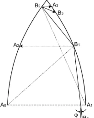
A Proof of theorem 1
of the cavity is the axis of the y and that its base A0A1 is placed on the axis
x. In this way, the position of the particle at entry of the cavity assumes only values in the interval−1
2, 1 2
× {0}.
x A1
A2 A3
A0 B1
B2
φ
x A1
A2 A3
A0 B1
B2
B3
φB0 B0
x A1
A2
A0 B1
B2
B3
φ
x A1
A2
A0 B1
B2
B3
φ φ+
(a) (b)
(d) (c)
B0 B4 B0
φ0
Fig. A.1. Set of illustrations to the study of the trajectory of particles with entry angle ϕ > ϕ0≃19.47◦, in the cavity “Double Parabola”.
Given the symmetry of the cavity in relation to its vertical axis, it will be enough to analyze its behavior for ϕ0 < ϕ < 90◦. The conclusions at which
we arrive will be in this way equally valid for −90◦ < ϕ <−ϕ
0.
We will analyze therefore in detail and separately each one of the sub-trajectories which compose all the trajectory described by the movement of the particle in the interior of the cavity.
Sub-trajectory −−−→B0B1
For ϕ > ϕ0, we have the guarantee that the first reflection occurs in the
parabolic curve of the left side of the cavity, just as can be easily deduced from the illustration (a). So that the particle collides with the left curve it is enough that the ϕ angle is superior to arctan(x/√2), a magnitude which has as upper boundϕ0 = arctan(
√
Sub-trajectory −−−→B1B2
After colliding in B1, in agreement with the law of reflection, the particle
follows trajectory−−−→B1B2. We prove that −−−→B1B2 has an ascendant path —
illus-tration (a). We trace the straight line A1A2, segment, parallel to the initial
trajectory of the particle B0B1, which passes through the focus of the left
parabola (A1). Because of the focal property of this parabola, a particle which
takes the sub-trajectory −−−→A1A2, after reflection at A2, will follow a horizontal
direction A2A3 (proceeding after its trajectory, after a new reflection, in the
direction of the focusA0 of the second parabola). Upon the occurrence of the
first reflection of the particle atB1, a point of the curve necessarily positioned
below A2, the trajectory −−−→B1B2, which it will follow straight away, will be on
an ascendant path, since the derivative dxdy of the curve at this point (B1) is
superior to the derivative inA2, where the trajectory followed was horizontal.
Although we now know that−−−→B1B2 takes an ascendant path, nothing yet
guar-antees to us that the second reflection happens necessarily in the parabola of the right side. If we are able to verify that forϕ =ϕ0 the second reflection is
always on the right side, no what the entry position x is, therefore, logically, the same will happen for any value ϕ > ϕ0. This premise can be easily
ac-cepted with the help of illustration (a) of figure A.2: for any value of ϕ > ϕ0,
with the first reflection at a given point B1, it is always possible to trace a
trajectory forϕ=ϕ0 which presents the first reflection at the same pointB1;
the second reflection at the curve of the right side being for the case ϕ=ϕ0,
necessarily the same will happen for the trajectory with ϕ > ϕ0, since the
angle of reflection will be less in this second case, just as is illustrated in the figure. Consequently, it will be enough for us to prove for ϕ = ϕ0, that the
second reflection always occurs in the parabola of the right side, so that the same is proven for any which is the ϕ > ϕ0.
(b)
B0
B2’
α
B1
θ β
φ0
θ
B2
α'
(a)
B0
A2
B1
φ0
B2
φ
Fig. A.2. Illustrations to the study of the second reflection.
conclude from the illustration, theB2 reflection only will happen on the curve
of the left side if theα angle is less than α′. We have determined the value of
the two angles.
Being (x1, y1) the coordinates of the pointB1, we will have tan(α′) =−x1/(
√ 2−
y1), thus
α′ = arctan −(y
2
1/4−1/2)
√ 2−y1
!
= arctan (2−y
2 1)/4
√ 2−y1
!
= arctan √
2 +y1
4
!
.
(A.1) In order to arrive at the value of α we resolve the system of three equations, of unknown α, θ and β, which are taken directly from the geometry of the actual figure
α+β+θ=π
β =ϕ0+θ
arctan12y1
+ϕ0+θ = π2
The tangent line to the curve in B1 makes with the vertical an angle whose
tangent has as its value the derivative dxdy of the curve at that point (iny =y1),
where dx dy = d dy( 1 4y
2−1 2) =
1
2y. Because of this, that angle emerges represented
in the third of the equations by the magnitude arctan(y1/2). By resolving the
system, the following result is obtained for α
α=ϕ0+ 2 arctan(y1/2) = arctan(
√
2/4) + 2 arctan(y1/2). (A.2)
Finally we prove that α > α′, no matter what y
1 ∈ (0,√2) is. Of the
equa-tions (A.2) and (A.1), it will be equivalent to proving
arctan(√2/4) + 2 arctan(y1/2)>arctan((
√
2 +y1)/4).
Given that 0< y1 <
√
2, both of the members of the inequality represent an-gles situated in the first quadrant of the trigonometrical circle. Because of this we can maintain the inequality for the tangent of the respective angles. Apply-ing the tangent to both of the members, after effectApply-ing some trigonometrical simplifications, we arrive at the following relation
1 4
4√2−√2y2
1 + 16y1
4−y2 1 −
√ 2y1
>
√ 2 +y1
4
Which, with additional algebraic simplifications, takes the form
y1 √
2y1+ 14 +y21
/(4−y12−√2y1)>0.
As 0< y1 <
√
Thus α > α′, which contradicts the condition which was necessary so that
the reflection B2 could occur on the curve of the left side, it therefore being
proven, as we intended, that in no situation does the reflectionB2 of
illustra-tion (b) of figure A.2 happen on the curve of the left side. Logically, we can therefore conclude that the same happens for whatever isϕ > ϕ0: the second
reflection of the particle occurs always in the parabola of the right side.
Sub-trajectory −−−→B2B3
We prove that the sub-trajectory −−−→B2B3 has a descendant path — illustration
(b) of figure A.1. Imagine, for this purpose, a sub-trajectory −−−→A0A2, parallel
to B1B2 and which passes through the focus A0. The sub-trajectory −−−→A2A3
which will follow the reflection in A2 — a point of the parabola on the right
side situated below B2 — will be horizontal. The derivative of the curve in
A2 being superior to the derivative value in B2, the sub-trajectoryB2B3 will
necessarily be of a descending nature.
Even if we already know that the sub-trajectory is descendant, we have not yet shown that sub-trajectory in no situation conducts the particle directly to the exit of the cavity. Therefore follows the proof that the reflectionB3 always
occurs in a position superior to A0 — illustration (c) of figure A.1. We trace
A2B2, a segment of the horizontal straight line which passes through the point
of reflectionB2. If the particle followed this trajectory, it would collide at the
same point B2, but heads itself toA0. Therefore, by the law of reflection,B3
will have to be above A0, since B1B2 makes an angle with the normal vector
at the curve in B2 less than that formed by segment A2B2.
Sub-trajectory −−−→B3B4
We will now show that the sub-trajectory which follows the reflection at B3
crosses the segment A0A1, that is, directs itself to the outside of the cavity
— illustration (d) of figure A.1. We trace, therefore,A2B3, a segment of
hor-izontal straight line which passes through the point of reflection B3. If the
particle followed this trajectory, it would collide at B3 and would head itself
towards A1. Therefore, by the law of reflection, the straight line where the
sub-trajectory −−−→B3B4 is placed will have necessarily to pass below A1, since
B2B3 makes an angle with the normal vector at the curve in B3 bigger than
that formed by the segment A2B3. We have shown that the sub-trajectory
crosses the axis of the xat a point situated to the left of A1, but we have not
yet shown that it occurs to the right of A0. For that, we will have to prove
that the third is the last of the reflections, that is, that in no situation does there occur a fourth reflection in the parabola of the left side. There follows this proof, of them all the most complex one.
collision in the left parabola, we will show that a fourth collision — represented byB4 in the illustration (a) of figure A.3 — has its origin always in an entry
angleϕ inferior toϕ0. We will thus study the trajectory of the particle in the
B3
α2
B4
α3
B2
θ3
θ3
β2
φ
α2
B2
θ1
θ2
θ2
B1
θ1
α1
B0
(b) (a)
Fig. A.3. Illustrations to the study of a hypothetical fourth reflection.
inverse order of its progression: we commence by admitting the existence of the sub-trajectory−−−→B3B4 of illustration (a) and we will analyze its implications
in all the preceding trajectory.
In illustration (a) of figure A.3 are to be found represented the sub-trajectories −−−→
B2B3and−−−→B3B4. We begin by relatingα2 withα3, the angles which the vectors
−−−→
B2B3 and −−−→B3B4, respectively, form with the vertical axis. For these purposes
we resolved the system of three equations, of unknown α2, θ3 and β2, which
are taken from the geometry of the figure,2
θ3 =β2+α3
arctan1 2y3
+β2 = π2
α2+θ3+β2 =π
obtaining
α2 = 2 arctan(y3/2)−α3,
in which arctan(y3/2) is the angle which the straight line tangent at the curve
in B3 makes with the vertical — the inclination of the straight line tangent
is given by dxdy |y=y3 =
d dy(
1 4y2 −
1
2)|y=y3 =
1
2y3. In its turn, the angle α3
can be expressed in the following way: α3 = arctan((x3−x4)/(y3 −y4)) =
arctan((14y2
3 −14y42)/(y3−y4)) = arctan((y3+y4)/4), which permits us to write
α2 in function only of the ordinates y3 and y4 of the extremes of the vector
−−−→
B3B4,
α2 = 2 arctan(y3/2)−arctan((y3+y4)/4). (A.3)
2 The variables denoted by x
In order to be able to prove what we intend — impossibility of occurrence of the reflection B4 — we need to find a lower bound for the ordinate of the
position where each one of the four reflections occurs, or in other words, to determine {y∗
1, y∗2, y∗3, y∗4}, just that
y1 ≥y1∗, y2 ≥y2∗, y3 ≥y3∗, y4 ≥y4∗, ∀(ϕ, x)∈(ϕ0, π/2)×(−1/2,1/2). (A.4)
It can easily be understood thaty∗
4 = 0. We will therefore determine the other
three lower bounds, commencing with y∗
2.
We know that 0< y4 < y3; therefore, from (A.3) we take away that
arctan(y3/2)< α2 <2 arctan(y3/2)−arctan(y3/4).
Being aware that α2 is situated in the first quadrant of the trigonometrical
circle, we can maintain the inequalities for the tangent of the respective angles. After some algebraic simplifications, we obtain
y3/2<tan(α2)< y3
12 +y32/16. (A.5)
The equation of the straight line which connects B2 to B3 takes the form
x=m(y−y3) +x3,withm = tan(α2) andx3 = 14y32−12. As we are interested
in finding the ordinate of the point of interception of this straight line with the parabolic curve situated on the right side, with equation x = −14y2 + 1
2,
we have to resolve the equation of second degree, in the variable y, which results in the elimination of the variablexby combination of the two previous equations. The ordinatey2, of the second reflection, being the positive root of
the equation, takes the formy2 =−2m+ q
4m2 + 4my
3−y32+ 4 .
The magnitude y2 is expressed in function of two variables, m and y3, which
as we know assume only positive values. So as to accept more easily the de-ductions which we are going to make in the tracking of y∗
2, we will imagine,
without any loss of generality, that y3 is a fixed value. We begin by showing
that the derivative of y2 in order to the variable m,
dy2
dm =
2
2m+y3− q
4m2+ 4my
3−y32+ 4
q
4m2+ 4my
3−y23+ 4
, (A.6)
has a negative value for whatever value ofy3 is. Asy3 <
√
2, inevitablyy2 3 <4,
thus the two radicands (4m2+4my
3−y32+4) present in the equation (A.6) have
always a positive value. The restrictiony3 <
√
2 allows us still to successively deduce the following inequalities
y23 <2⇔2y32 <4⇔y23 <4−y32 ⇔4m2+ 4my3+y23 <4m2+ 4my3+ 4−y23
⇔(2m+y3)2 <4m2+ 4my3−y32+ 4⇔2m+y3 < q
4m2 + 4my
This last inequality confirms that dy2
dm <0, for whatevery3 may be. In this way,
the value y2 is so much less the greater is the value of m. As is examined in
(A.5), m < M =y3(12 +y23)/16, thus y2 >−2M+ q
4M2+ 4M y
3−y23 + 4 .
SubstitutingM, there is obtained, after some simplifications,
y2 > f(y3), with f(y3) = −
3 2y3 −
1 8y 3 3 + 1 8 q
272y2
3 + 40y34+y36+ 256 . (A.7)
In order to find the minimum value off(y3) we begin by computing its
deriva-tive:
d dy3
f(y3) =
272y3+ 80y33 + 3y53−(12 + 3y23) q
272y2
3 + 40y34+y36+ 256
8q272y2
3 + 40y43 +y63+ 256
.
The radicands being clearly positive, we only have to concern ourselves with the numerator of the fraction. To find the roots of the derivative function
d
dy3f(y3) is equivalent because of this to resolving the equation
272y3+ 80y33+ 3y53 2
=12 + 3y232272y32+ 40y43+y63+ 256,
which can be simplified in the following:
2304−1024y23−992y34−160y63−3y83 = 0.
This polynomial equation has only one real positive root, of the value ˜y3 = 2
3 q
−51 + 6√79 ≃ 1.017, signifying that f(y3) has a global minimum in ˜y3,
because, as we show in what follows, d2
dy2
3f(y3)> 0 and the function does not presents other points of stationarity.
We thus show that d2
dy2
3f(y3)>0, with
d2
dy2 3
f(y3) =
18240y4
3 + 2960y36+ 180y38+ 3y310+ 34816 + 30720y32
4(272y2
3 + 40y43+y63+ 256)
3 2
−(816y
3
3 + 120y35+ 3y73 + 768y3) q
272y2
3 + 40y34+y36+ 256
4(272y2
3 + 40y34+y36+ 256)
3 2
. (A.8)
We show that d2
dy2
3f(y3) > 0 is equivalent to showing that the numerator of the first fraction is superior to the numerator of the second, in (A.8). After elevating the two terms to the square, we arrive at the inequality
−3y316+ 36y314+ 9464y312+ 191616y310+ 1514112y38+ 5817344y63
We easily prove the veracity of this relation, given that we have a unique negative term (−3y16
3 ) which, for example, is inferior in absolute value to the
constant term (9469952), y3 <
√
2 ⇒ 3y16
3 < 768 < 9469952. The proof is
thus complete that f(y3) has a global minimum in ˜y3, of the value f(˜y3) = 8
9 q
−51 + 6√79.
Accordingly, from (A.7), we finally conclude that
y2 > y∗2 =
8 9
q
−51 + 6√79≃1.356. (A.9)
A lower bound is then found for the height of the second reflection B2
(illus-tration (a) of figure A.3). We now determiney∗
3, a lower bound for the height
of the third reflection B3.
So that the reflectionB2 occurs in the parabola of the right side it is necessary
that the angle α2 is greater than the angle formed between the vertical axis
and the segment of straight line which unites B3 with the superior vertex of
the cavity,
α2 >arctan
−x3
√ 2−y3
= arctan
−1 4y
2 3 +12
√ 2−y3
= arctan
√2 +y 3
4
. (A.10)
This inequality, in conjunction with the second relation of inequality of (A.5), allows us to write
(√2 +y3)/4<tan(α2)< y3
12 +y23/16⇒(√2 +y3)/4< y3
12 +y32/16,
from which results the inequality
y33+ 8y3+ 4
√
2>0. (A.11)
As the polynomial of the left hand-side of (A.11) has a positive derivative and admits a unique real root, we immediately conclude that it constitutes an inferior limit for y3, this limit being
y∗
3 =
1 3
54√2 + 6√546 1 3
−854√2 + 6√546 −1
3
≃0.670. (A.12)
It is left to us to determine y∗
1, a lower bound for the value of y1 — the
ordinate where the first reflection occurs. To this end we resort to illustration (b) of figure A.3, which gives us a more detailed representation of the part of the cavity where the first two reflections occur, B1 and B2. The scheme
presented was constructed counting that the first reflection (B1) occurs at a
point which is more elevated than that of the third reflection (B3). This is
in fact the situation. This itself can be proven by showing that α2 is always
smaller than the angle formed between the normal vector at the curve in B2
and the vertical axis, or that isα2 < π2 −arctan
1 2y2
Taking, in (A.5), at the upper limit of tan(α2) and having in mind thaty <
√ 2, we build the following sequence of inequalities which proves what is intended:
α2 <arctan
y3(12 +y32)
16
!
<
≃51.06◦
z }| {
arctan 7 √ 2 8 ! <
≃54.74◦
z }| {
π
2 −arctan √
2 2
!
< π
2−arctan
1
2y2
.
We now try to find y∗
1. We can define y1∗ as being the ordinate of the point
of interception of the left parabola with the semi-straight line with its origin at point B2, positioning as low as possible (y2 = y2∗), and with equal slope
to the largest value permitted for the slope of the trajectory which preceded
B2 (−−−→B1B2). The equation of the straight line which connects B1 to B2 takes
the form x = m(y−y2) +x2, with m = tan(α1) and x2 = −14y22 +12. As we
are interested in finding the point of intersection of this straight line with the parabolic curve situated on the left side, with equation x= 1
4y 2 −1
2 , we will
have to resolve the equation of the second degree, in the variable y, which results in the elimination of the variablexby combination of the two previous equations. Although we have two positive real roots, we are only interested in the smaller of the two, which takes the form
y1 = 2m− q
4m2−4my
2−y22+ 4 . (A.13)
As we said, if we do y2 = y2∗ and place the maximum slope to the straight
line, which in the previous equations is equivalent to consideringmminimum, we obtain y1 = y∗1. Being m = tan(α1), we should determine the value of α1
through the system of equations
α1 = 2θ2+α2
arctan1 2y2
+α2+θ2 = π2
which is taken from the geometry of illustration (b) of figure A.3. Is obtained
α1 =π−2 arctan(y2/2)−α2. (A.14)
From this latest equality, from (A.5), and given that y2 <
√
2 and y3 <
√ 2, we deduce that α1 > π −2 arctan(y2/2) − arctan(y3(12 +y32)/16) > π −
2 arctan(1/√2)−arctan(7√2/8), thusm = tan(α1)>tan(π−2 arctan(1/
√ 2)− arctan(7√2/8)) = 23
20
√
2. If in (A.13) we do m = 23 20
√
2 and y2 = y∗2 we then
obtain the inferior limit fory1
y∗1 = 23 10
√ 2− 1
90
r
444498−33120√2
q
−51 + 6√79−38400√79≃1.274. (A.15) Summarizing, (y∗
With the help of illustration (b) of figure A.3 we will, finally, analyze the entry angle ϕ of the particle. With the system of equations (1
2y1 = dx dy |y=y1)
2θ1+ϕ+α1 =π
arctan1 2y1
+ϕ+θ1 = π2
and with equalities (A.14) and (A.3) we obtain, successively,
ϕ=α1−2 arctan(y1/2),
ϕ=π−2 arctan(y1/2)−2 arctan(y2/2)−α2, (A.16)
ϕ=π−2 arctan(y1/2)−2 arctan(y2/2)−2 arctan(y3/2) + arctan((y3+y4)/4).
Taking (A.16), from (A.10) we deduce thatϕ < π−2 arctan (y1/2)−2 arctan (y2/2)−
arctan((√2 +y3)/4). In agreement with the definitions (A.4) and with the
val-ues found in (A.9), (A.12) and (A.15), we can conclude that
ϕ < π−2 arctan(y1∗/2)−2 arctan(y2∗/2)−arctan((√2 +y3∗)/4)≃19.18◦,
or that is
ϕ < ϕ0 ≃19.47◦.
With this we can finally conclude that it is impossible to have a fourth reflec-tion, since for this to happen the particle would have to have entered in the cavity with an angle ϕ < ϕ0, as we have just finished showing — something
which would contradict our initial imposition, ϕ > ϕ0. As the cavity presents
symmetry in relation to its central vertical axis, the conclusion to which we have arrived is equally valid for ϕ < −ϕ0, thus being proven that which we
intended (theorem 1):
For |ϕ| > ϕ0, there always occur three reflections, alternatively on the left
and right facets of the Double Parabola cavity.
B Proof of theorem 2
For |ϕ| > ϕ0 the statement of theorem 2 is already proved. It remains to
consider the case−ϕ0 < ϕ < ϕ0, but given the symmetry of the cavity we will
only need to study the interval 0< ϕ < ϕ0.
For 0< ϕ < ϕ0 the first reflection can just as well occur on the left-hand facet
as on the right-hand side. We will analyze each one of the cases separately.
1st reflection on the left-hand side
Being 0 < ϕ < ϕ0 we can have the first two reflections on the left-hand
facet, it being in this case guaranteed, as we assume above, that 3 or more reflections will exist. If on the other hand, the second reflection is on the right side, an initial part of the trajectory can always be represented by the first three illustrations of figure A.1 (assuming 0< ϕ < ϕ0), which guarantee, also
in this case, the existence of a third reflection B3. In order to prove what we
have just finished saying, it will be enough to prove the ascendant nature of the sub-trajectory−−−→B1B2.
We establish on the parabola of the left side (illustration (a) of figure A.1) the first point of reflection B1. For whatever B1 is it is always possible for us to
trace an initial sub-trajectory −−−→B0B1 with its origin in an entry angle ϕ > ϕ0.
As in appendix A (page 17) we showed the sub-trajectory −−−→B1B2 which would
follow it to be ascendant, the same will necessarily come about for whatever 0 < ϕ < ϕ0 may be, given that in this case −−−→B0B1 will represent a more
accentuated negative slope. Since in appendix A (page 19) we characterized −−−→
B2B3 only with basis in the ascendant nature of the sub-trajectory preceding
−−−→
B1B2, the conclusions to which we arrive for −−−→B2B3 are equally valid for 0 <
ϕ < ϕ0.
1st reflection on the right side
Also in this case we can have the first two reflections on the right-hand facet, it being guaranteed that 3 or more reflections will exist. If this does not occur, we will necessarily have a trajectory with the aspect of the trajectoryB0B1B2B3
illustrated in the scheme of figure B.1, where as well there are represented two auxiliary trajectories (the dotted lines),A0B1A2 and A1B2A3, which, on
passing through the foci of the parabolas, present the sub-trajectory posterior to the reflection horizontal. Having as a basis the laws of reflection, we can succinctly deduce the following: as the angleA\0B1A2 must be interior to the
angleB\0B1B2, we conclude that−−−→B1B2 is of a ascendant nature; asB\1B2B3 is
necessarily an interior angle toA\1B2A3, we conclude thatB3 must be situated
betweenA1 and A3, which guarantees the existence of a third reflection. Thus
A1 A2
A3
A0
B1 B2
B0 B3
φ
Fig. B.1. Illustrative scheme to the study of the trajectory of particles with entry angle 0< ϕ < ϕ0.
Acknowledgements
This work was supported by the Centre for Research on Optimization and
Control (CEOC) from thePortuguese Foundation for Science and Technology
(FCT), cofinanced by the European Community Fund (ECF) FEDER/POCI 2010; and by the FCT research project PTDC/MAT/72840/2006.
References
[1] Isaac Newton. Philosophiae naturalis principia mathematica. (London: Streater), 1687.
[2] G. Buttazzo, V. Ferone, and B. Kawohl. Minimum problems over sets of concave functions and related questions. Math. Nachr., 173:71–89, 1995.
[3] G. Buttazzo and P. Guasoni. Shape optimization problems over classes of convex domains. J. Convex Anal., 4(2):343–351, 1997.
[4] G. Buttazzo and B. Kawohl. On Newton’s problem of minimal resistance. Matth. Intell., 15:7–12, 1993.
[5] T. Lachand-Robert and E. Oudet. Minimizing within convex bodies using a convex hull method. SIAM J. Optim., 16:368–379, 2006.
[6] T. Lachand-Robert and M. A. Peletier. An example of non-convex minimization and an application to Newton’s problem of the body of least resistance. Ann. Inst. H. Poincar, Anal. Non Lin., 18:179–198, 2001.
[7] F. Brock, V. Ferone, and B. Kawohl. A symmetry problem in the calculus of variations. Calc. Var., 4:593–599, 1996.
[9] T. Lachand-Robert and M. A. Peletier. Newton’s problem of the body of minimal resistance in the class of convex developable functions. Math. Nachr., 226:153–176, 2001.
[10] Alexander Yu. Plakhov. Newtons problem of a body of minimal aerodynamic resistance. Dokl. Akad. Nauk., 390(3):314–317, 2003.
[11] Alexander Yu. Plakhov. Newton’s problem of the body of minimal resistance with a bounded number of collisions. Russ. Math. Surv., 58(1):191–192, 2003.
[12] Alexander Yu. Plakhov. Newton’s problem of the body of minimum mean resistance. Sbornik: Mathematics, 195(7–8):1017–1037, 2004.
[13] D. Horstmann, B. Kawohl, and P. Villaggio. Newton’s aerodynamic problem in the presence of friction. Nonlin. Differ. Eq. Appl., 9:295–307, 2002.
[14] Alexander Yu. Plakhov and Delfim F. M. Torres. Newton’s aerodynamic problem in a medium of chaotically moving particles. Sbornik: Mathematics, 196(6):111–160, 2005.
[15] Alexander Yu. Plakhov Billiards and two-dimensional problems of optimal resistance.Arch. Ration. Mech. Anal., DOI 10.1007/s00205-008-0137-1 (33 pp.), 2008.
[16] Alexander Yu. Plakhov and Paulo D. F. Gouveia. Bodies of maximal aerodynamic resistance on the plane. Cadernos de Matem´atica, CM07/I-12, Universidade de Aveiro, Abril 2007.
[17] Alexander Yu. Plakhov and Paulo D. F. Gouveia. Problems of maximal mean resistance on the plane. Nonlinearity, 20:2271–2287, 2007.
[18] Brian W. Kernighan and Dennis M. Ritchie. The C Programming Language. Prentice-Hall, second edition, 1988.
[19] Genetic algorithm and direct search toolbox user’s guide – for use with MATLAB. The MathWorks, Inc., 2004.
[20] D. G. Hook and P. R. McAree. Using sturm sequences to bracket real roots of polynomial equations. In Graphics gems, pages 416–422. Academic Press Professional, Inc., San Diego, CA, USA, 1990.