The Exponentiated Power Generalized Weibull: Properties and Applications

(Annals of the Brazilian Academy of Sciences)

Printed version ISSN 0001-3765 / Online version ISSN 1678-2690 http://dx.doi.org/10.1590/0001-3765201820170423

www.scielo.br/aabc | www.fb.com/aabcjournal

The Exponentiated Power Generalized Weibull: Properties and Applications

FERNANDO A. PEÑA-RAMÍREZ1_{, RENATA R. GUERRA}1_{, GAUSS M. CORDEIRO}2_{and PEDRO R.D. MARINHO}3

1_{Departamento de Estatística, Universidade Federal de Santa Maria, Cidade Universitária,} Av. Roraima, 1000, 97105-900 Santa Maria, RS, Brazil

2_{Departamento de Estatística, Universidade Federal de Pernambuco, Cidade Universitária,} Av. Prof. Moraes Rego, 1235, 50740-540 Recife, PE, Brazil

3_{Departamento de Estatística, Universidade Federal da Paraíba, Cidade Universitária,} Conj. Pres. Castelo Branco III, s/n, 58051-900 João Pessoa, PB, Brazil Manuscript received on June 20, 2017; accepted for publication on November 1, 2017

ABSTRACT

We propose a new lifetime model called the exponentiated power generalized Weibull (EPGW) distribu-tion, which is obtained from the exponentiated family applied to the power generalized Weibull (PGW) distribution. It can also be derived from a power transform on an exponentiated Nadarajah-Haghighi ran-dom variable. Since several structural properties of the PGW distribution have not been studied, they can be obtained from those of the EPGW distribution. The model is very flexible for modeling all common types of hazard rate functions. It is a very competitive model to the well-known Weibull, exponentiated expo-nential and exponentiated Weibull distributions, among others. We also give a physical motivation for the new distribution if the power parameter is an integer. Some of its mathematical properties are investigated. We discuss estimation of the model parameters by maximum likelihood and provide two applications to real data. A simulation study is performed in order to examine the accuracy of the maximum likelihood estimators of the model parameters.

Key words:Exponential distribution, lifetime data, Nadarajah-Haghighi distribution, power generalized Weibull distribution, survival function.

1 - INTRODUCTION

There has been an increased interest in defining new continuous distributions by adding shape parameters to an existing baseline model. One of the most widely-accepted methods on this parameter induction is the exponentiated-G (exp-G) class. LetG(y)andg(y)be the baseline cumulative distribution function (cdf) and

the probability density function (pdf) of a random variableW, respectively. We obtain the exp-G cdf by

raisingG(y)to a positive power shape parameter to the baseline model. Thus, a random variableY has an

exp-G distribution if its cdf is given by

F(y) =G(y)β,

fory∈D_⊆R, where_β>0represents the additional parameter. The corresponding pdf is given by

f(y) =βg(x)G(y)β−1.

Tahir and Nadarajah (2015) traced this approach back to the first half of the nineteenth century and found twenty-eight different exp-G models published in recent literature. Most of these models are motivated by their usefulness in exploring tail properties and also for improving the goodness-of-fit in comparison with their baselines. Another current reason for introducing exp-G distributions is their applications in lifetime data analysis.

Thus, the classical lifetime distributions have received a great deal of attention as baselines on the exp-G class, among other generated families. Using the exponential lifetime model as baseline, Gupta et al. (1998) pioneered the exponentiated exponential (EE) distribution.

The exponentiated Weibull (EW) distribution was introduced by?.

Another model that has been considered for modeling lifetime data is the Nadarajah-Haghighi (NH) dis-tribution pioneered by Nadarajah and Haghighi (2011). The NH model is a generalization of the exponential distribution with cdf given by (forz>0)

G(z) =1−exp{1−(1+λz)α}, (1)

whereλandαare the scale and shape parameters, respectively. IfZhas the cdf (1), we writeZ∼NH(α,λ).

The pdf ofZis given by

g(z) =αλ(1+λz)α−1exp{1−(1+λz)α}. (2)

The motivations for studying the NH model are: the relationship between the pdf (2) and its hazard rate func-tion (hrf), the ability (or inability) to model data with mode fixed at zero and the fact that it can be interpreted as a truncated Weibull distribution. Further details and general properties can be found in Nadarajah and Haghighi (2011). The exponentiated Nadarajah-Haghighi (ENH) model was proposed by Lemonte (2013). The exponential, NH and Weibull distributions are all special cases of the power generalized Weibull (PGW) distribution proposed by Bagdonavicius and Nikulin (2002) in the context of accelerated failure time models. The original PGW cdf is given by (fort>0)

G(t) =1−e1− h

1+ t σ

βi1γ ,

whereσ,β andγ>0. By settingλ =σ−β andα=γ−1, the cdf, pdf and hrf of this distribution reduce to

G(t) =1−exp{1−(1+λtγ)α}, (3)

g(t) =αλ γtγ−1(1+λtγ)α−1exp{1−(1+λtγ)α} (4) and

respectively. Dimitrakopoulou et al. (2007) presented a lifetime model that has the same formulation as that one in (3) with motivation in competing risk scenario. Lai (2013) described the PGW among the Weibull generalizations that are often required to prescribe the nonmonotonic nature of the empirical hazard rates.

Nikulin and Haghighi (2006) introduced a chi-square statistic for testing the validity of the PGW dis-tribution and presented an application to censored survival times of cancer patients. Nikulin and Haghighi (2009) presented shape analysis for the PGW pdf and hrf. They also obtained a series representation for the

sth moment of this distribution, but only for integer values ofs/γ. They do not provide a general expression

for the PGW ordinary moments. We also note that there is a lack of other structural properties of the PGW distribution like incomplete moments, skewness, mean deviations, Bonferroni and Lorenz curves and Rényi entropy.

In this paper, we use the concept of exponentiated distributions for introducing a new four-parameter Weibull-type family, so-called theexponentiated power generalized Weibull(EPGW) distribution. The pro-posed distribution is obtained by considering the PGW model as baseline in the exp-G family. Thus, the EPGW cdf and pdf are given by (fort>0)

F(t) = [1−exp{1−(1+λtγ)α}]β, (5)

and

f(t) =αβ λ γtγ−1(1+λt

γ₎α−1_{exp{1−(1+λt}γ₎α_}

[1−exp{1−(1+λtγ)α_}]1−β , (6)

respectively. Here,λ is the scale parameter andγ,α andβ are shape parameters. Henceforth, we denote by T a random variable having pdf (6), sayT ∼EPGW(α,β,λ,γ). Identifiability is a property which a model

must satisfy for precise inference to be possible, which refers to whether the unknown parameters in the model can be uniquely estimated. Equation (5) is clearly identifiable.

The hrf ofT is given by

h(t) =αβ λ γtγ−1(1+λtγ)α−1

×exp{1−(1+λt

γ₎α_{}[1−exp{1−(1+λt}γ₎α_}]β−1

1−[1−exp{1−(1+λtγ)α_}]β . (7)

By inverting (5), we obtain an explicit expression for the quantile function (qf) of the EPGW distribution, sayQ(u), given by

Q(u) =λ−1/γh1−log(1−u1/β)i1/α−1

1/γ

, u∈(0,1). (8)

Its medianMfollows by settingu=1/2in (8). The simulation of the EPGW random variable is

straight-forward. IfU ∼U(0,1), then the random variable T =Q(U) follows the EPGW distribution given by

(6).

Some motivations for introducing the EPGW distribution are:

TABLE I

Some special models of the EPGW distribution.

α β λ γ Distribution

1 1 - 1 Exponential

1 - - 1 Exponentiated exponential

1 1 - 2 Rayleigh

1 - - 2 Burr type X

1 1 - - Weibull

1 - - - Exponentiated Weibull

- 1 - 1 Nadarajah-Haghighi

- - - 1 Exponentiated Nadarajah-Haghighi - 1 - - Power generalized Weibull

• The current distribution can also be derived from a power transform on an ENH random variable. If

Y ∼ENH(α,β,λ), the cdf ofY is given by

FY(y) = [1−exp{1−(1+λy)α}]β, y>0,

whereα >0, β >0andλ >0. Consider the transformationT =Y1/γ, where γ>0. Thus, the cdf

ofT has the form F(t) =FY(tγ) given by (5). A similar approach was addressed by Gomes et al.

(2008). They proposed a new method of estimation for the generalized gamma distribution through the power transformationW =Xc, whereX is a generalized gamma random variable andW has the

gamma distribution.

• Once several structural properties of the PGW distribution have not been studied, they shall be obtained from those of the EPGW distribution.

• By pioneering a PGW generalization of the exp-G family, it is also possible to obtain several proper-ties of other generated families based on linear combinations from those of the EPGW distribution. For example, for the beta-G famil (Eugene et al. 2002), the density function can be expressed as a linear combination of exp-G pdfs for any baseline G. Similar results can also be demonstrated for the Kumaraswamy-G introduced by Cordeiro and Castro (2011), among several others generated families of distributions.

• Letβ>0be an integer. Thus,F(t)given in (5) represents the cdf of the maximum value on aβ-variate

random sample from the PGW distribution, say:T =max{T1, . . . ,Tβ}. In other words, the EPGW distribution can be used to model the maximum lifetime of a random sample from the PGW distribution with sizeβ. Further, as part of the exp-G family, the EPGW distribution has the following physical

interpretation. Consider a parallel system consisting ofβ=ncomponents, which means that the system

works if at least one of then-components works. If the lifetime distributions of the components are

• The EPGW may provide consistently ‘better fits’ than other Weibull generalizations including its spe-cial models. This fact is shown by fitting the proposed distribution to two data sets in Section 13. The applications illustrate that the EPGW distribution can also be very competitive to other widely known lifetime models.

The paper is outlined as follows. Some mathematical properties of the new distribution are provided in Sections 3-10. They include ordinary and incomplete moments, mean deviations about the mean and the median, Bonferroni and Lorenz curves, Rényi entropy, reliability and order statistics. In Section 11, we present the maximum likelihood method to estimate the model parameters. In Section 12, a simulation study evaluates the performance of the maximum likelihood estimators (MLEs). Applications to two real data sets are presented in Section 13. Section 14 offers some concluding remarks.

2 - DENSITY AND HAZARD SHAPES

Note that the pdf (6) can be expressed in terms of the cdf and pdf given in (3) and (4), respectively, in the form f(t) =βG(t)β−1g(t). Thus, the multiplicative factorβG(t)β−1is greater (smaller) than one forβ >1

(β<1)and for larger values oft, and the opposite occurs for smaller values oft. The inclusion of the extra

shape parameterβ provides greater flexibility in terms of skewness and kurtosis of the new distribution.

The pdf (6) can take various forms depending on the values of the shape parametersα,β andγ. It is easy to

verify that

lim t→0f(t) =

      

∞ ifβ <1, αλ γ ifβ =1,

0 ifβ >1,

andlimt→∞f(t) =0.

Setingz= (1+λtγ)α, we can rewrite the EPGW pdf as

ψ(z) =αβ λ1/γγz(α−1)/α(z1/α−1)(γ−1)/γe1−z(1−e1−z)β−1.

Differentiating twicelogψ(z)with respect toz, we obtain

d2logψ(z)

dz2 =−

"

α−1

αz2 +

(β−1)e1−z

(1−e1−z₎2 +

zα1−2(γ−₁)₁+α _z1/α−₁ α2_{γ z}1/α₋₁2

#

.

Note thatz= (1+λtγ)α implies thatz>1. Thus, we can verify that fort>0, α <1,β <1 andγ <1,

[d2logψ(z)/dz2]>0. This implies that the EPGW pdf is log-convex. Further, fort>0,α >1,β >1and

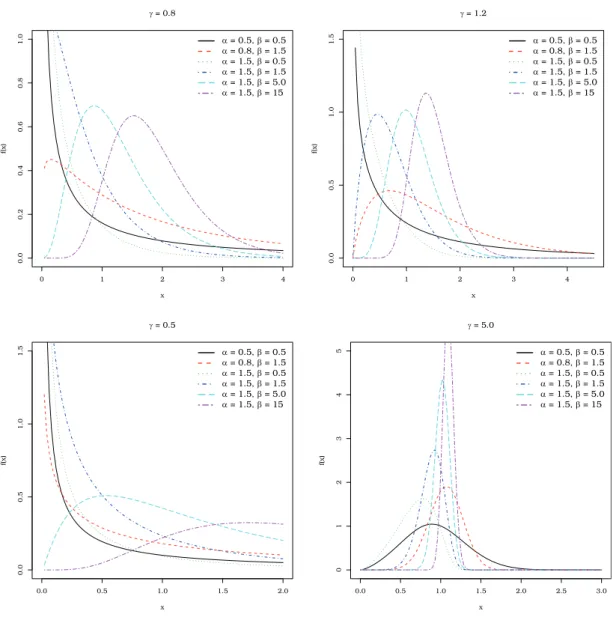
γ>1,[d2logψ(z)/dz2]<0, which implies that the EPGW pdf is log-concave. Figure 1 displays plots of the

pdf (6) for some parameter values. It illustrates the flexibility of the EPGW density, which allows modeling skewed and asymmetrical data.

Analogously, the EPGW hrf can be rewritten as

φ(z) =αβ λ1/γγz(α−1)/α(z1/α−1)(γ−1)/γe

1−z_(1−e1−z₎−1

(1−e1−z)−β₋₁. The critical point are obtained from

d logφ(z)

dz =

α−1

αz +

(γ−1)z(1−α)/α αγ(z1/α−1) +

βe1−z

(1−e1−z)[1−(1−e1−z)β_]−

e1−z

0 1 2 3

0.0

0.2

0.4

0.6

0.8

1.0

g = 0.8

x

f(x)

a = 0.5, b = 0.5

a = 0.8, b = 1.5

a = 1.5, b = 0.5

a = 1.5, b = 1.5

a = 1.5, b = 5.0

a = 1.5, b = 15

4 0 1 2 3 4

0.0

0.5

1.0

1.5

g = 1.2

x

f(x)

a = 0.5, b = 0.5

a = 0.8, b = 1.5

a = 1.5, b = 0.5

a = 1.5, b = 1.5

a = 1.5, b = 5.0

a = 1.5, b = 15

0.0 0.5 1.0 1.5 2.0

0.0

0.5

1.0

1.5

g = 0.5

x

f(x)

a = 0.5, b = 0.5 a = 0.8, b = 1.5 a = 1.5, b = 0.5 a = 1.5, b = 1.5 a = 1.5, b = 5.0 a = 1.5, b = 15

0.0 0.5 1.0 1.5 2.0 2.5 3.0

0

1

2

3

4

5

g = 5.0

x

f(x)

a = 0.5, b = 0.5 a = 0.8, b = 1.5 a = 1.5, b = 0.5 a = 1.5, b = 1.5 a = 1.5, b = 5.0 a = 1.5, b = 15

Figure 1 -Plots of the EPGW density forλ=1.

Forα=β =γ=1,d logφ(z)/dz=0and the hrf is constant. Forα<1,γ<1andβ<1,d logφ(z)/dz<0

and the hrf is decreasing. There may be more than one root to this equation.

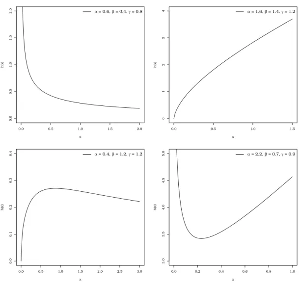
Figure 2 provides plots of the hrf (7) for some parameter values. Figure 2 reveals that the EPGW distri-bution can have decreasing, increasing, upside-down bathtub and bathtub-shaped hazard functions. This fea-ture makes the new distribution very attractive to model lifetime data. For example, according to Nadarajah et al. (2011) most empirical life systems have bathtub shapes for their hrfs.

3 - MOMENTS

Thesth ordinary moment ofT is obtained asE(Ts) =R₀∞tsf(t)dt, with f(t)from (6). For illustrative

0.0 0.5 1.0 1.5 2.0

0.0

0.5

1.0

1.5

2.0

x

h(x)

a = 0.6, b = 0.4, g = 0.8

0.0 0.5 1.0 1.5

0

1

2

3

4

x

h(x)

a = 1.6, b = 1.4, g = 1.2

0.0 0.5 1.0 1.5 2.0 2.5 3.0

0.0

0.1

0.2

0.3

0.4

x

h(x)

a = 0.4, b = 1.2, g = 1.2

0.0 0.2 0.4 0.6 0.8 1.0

3.0

3.5

4.0

4.5

5.0

x

h(x)

a = 2.2, b = 0.7, g = 0.9

Figure 2 -Plots of the EPGW hrf forλ=1.

These results are presented in Table II. All computations are obtained usingR software, which have numerical integration routines with great precision. Based on these values, we can note that, for fixedγ,

the additional parameterβ has large impact on the moments ofT. Note that the moments increase as β

increases. Forβ fixed and≤1, the moments decreases whenγincreases.

Thesth moment ofT can also be determined from equation (8). After some algebra, we can write

µ_s′=IE(Ts) =β λ−s/γIs(α,β,γ),

whereIs(α,β,γ) = R1

0{[1−log(1−u)]1/α−1}s/γuβ−1duis an integral to be evaluated numerically.

Using the binomial expansion since0<e1−(1+λtγ)α _{<1,the inverse of the denominator of (6) can be}

expressed as

[1−exp{1−(1+λtγ)α}]β−1=

∞

∑

(−1)j

β−1

j

Further, we can rewriteµ_s′as

µ_s′=αβ λ γ

∞

∑

(−1)j

β−1

j

ej+1

Z ∞

0

ts+γ−1(1+λtγ)α−1e−(j+1)(1+λtγ)αdt. (9)

We consider the integral

J=

Z ∞

0 t

s+γ−1_(1+λtγ₎α−1_e−(j+1)(1+λtγ)α_dt.

Settingu= (j+1)(1+λtγ)α, we have

t=

(

λ−1

"

u j+1

1/α

−1

#)1/γ

.

Hence, after some algebra, we obtain

J=

1

λ

s/γZ _∞

j+1 "

u j+1

1/α

−1 #s/γ

e−u

αλ γ(j+1)du. (10)

The most general case of the binomial theorem is the power series identity

(x+a)ν=

∞

∑

ν k

xkaν−k, (11)

where ν

k

is a binomial coefficient andν is a real number. This power series converges forν ≥0an

in-teger, or |x/a|<1. This general form is given by Graham (1994). By using (11) in equation (10), since

[u/(j+1)]1/α<1, it follows from (9) that

µ_s′=β λ−s/γ

∞

∑

(−1)i+j_ej+1

(j+1)[s−γ(i−α)]/αγ

_β −1 j s/γ i Γ

s−γ(i−α) αγ , j+1

, (12)

whereΓ(a,x) =R_x∞za−1e−zdzdenotes the complementary incomplete gamma function, which is defined for

all real numbers except the negative integers. Equation (12) is the main result of this section.

4 - SKEWNESS

The central moments(µs)and cumulants(κs)ofT can be expressed recursively from equation (12) as

µs= s

∑

(−1)k

s k

µ₁′kµ_s−k′ and κs= s−1

∑

s−1

k−1

κkµs−k′ ,

respectively, whereκ1=µ1′. Thus,κ2=µ2′−µ1′2,κ3=µ3′−3µ2′µ1′+2µ1′3, etc. The skewnessγ1=κ3/κ 3/2 2

and kurtosisγ2=κ4/κ22can be determined from the third and fourth standardized cumulants.

The MacGillivray (1986) skewness function ofT is given by

ρ(u) =ρ(u;α,β,γ) =ρ(1)(u;α,β,γ) ρ₍₂₎(u;α,β,) =

TABLE II

First six moments for some scenarios ofγandβ, with fixedα=1.5andλ=1.

γ β E(T) E(T2_{) E(T}3_{) E(T}4_{) E(T}5_{) E(T}6₎

0.5

0.5 0.2989 0.6249 2.7433 19.2657 191.2419 2498.7853 0.8 0.4488 0.9827 4.3653 30.7679 305.7880 3997.1257 1.0 0.5397 1.2149 5.4372 38.4129 382.0702 4995.6341 2.0 0.9176 2.3100 10.6904 76.3690 762.5177 9983.6001 3.0 1.2116 3.3145 15.7832 113.8992 1141.4011 14964.0482 4.0 1.4537 4.2472 20.7336 151.0300 1518.7741 19937.1200

0.8

0.5 0.3162 0.3259 0.5425 1.2207 3.4227 11.4158 0.8 0.4515 0.4986 0.8507 1.9344 5.4503 18.2210 1.0 0.5278 0.6062 1.0498 2.4030 6.7917 22.7400 2.0 0.8109 1.0755 1.9810 4.6677 13.3819 45.1295 3.0 1.0030 1.4633 2.8250 6.8184 19.7945 67.1961 4.0 1.1481 1.7964 3.6014 8.8727 26.0480 88.9632

1.0

0.5 0.3450 0.2989 0.3824 0.6249 1.2207 2.7433 0.8 0.4789 0.4488 0.5924 0.9827 1.9344 4.3653 1.0 0.5517 0.5397 0.7257 1.2149 2.4030 5.4372 2.0 0.8066 0.9176 1.3275 2.3100 4.6677 10.6904 3.0 0.9688 1.2116 1.8477 3.3145 6.8184 15.7832 4.0 1.0868 1.4537 2.3092 4.2472 8.8727 20.7336

2.0

0.5 0.4818 0.3450 0.3012 0.2989 0.3259 0.3824 0.8 0.6092 0.4789 0.4391 0.4488 0.4986 0.5924 1.0 0.6702 0.5517 0.5194 0.5397 0.6062 0.7257 2.0 0.8518 0.8066 0.8308 0.9176 1.0755 1.3275 3.0 0.9488 0.9688 1.0538 1.2116 1.4633 1.8477 4.0 1.0129 1.0868 1.2278 1.4537 1.7964 2.3092

3.0

0.5 0.5773 0.4186 0.3450 0.3099 0.2968 0.2989 0.8 0.6929 0.5504 0.4789 0.4459 0.4377 0.4488 1.0 0.7445 0.6168 0.5517 0.5234 0.5210 0.5397 2.0 0.8868 0.8277 0.8066 0.8158 0.8527 0.9176 3.0 0.9571 0.9482 0.9688 1.0181 1.0976 1.2116 4.0 1.0018 1.0306 1.0868 1.1725 1.2925 1.4537

4.0

whereu∈(0,1),Q(·)is the qf defined in (8),

ρ₍₁₎(u;α,β,γ) = h1−log(1−(1−u)1/β)i1/α−1

1/γ

+h1−log(1−u1/β)i1/α−1

1/γ

− 2h1+β−1log(2)−log(21/β−1)i1/α−1

1/γ

and

ρ₍₂₎(u;α,β,γ) = h1−log(1−(1−u)1/β)i1/α−1

1/γ

−h1−log(1−u1/β)i1/α−1

1/γ

.

It is based on quantiles and can illustrate the effects of the shape parametersα,β andγ on the skewness

ofT. Plots ofρ(u)for some parameter values are displayed in Figure 3. These plots reveal that when the

parametersβ andγ increase, the functionρ(u)converges to zero. The closerρ(u)is to the horizontal line ρ(u) =0, the density becomes more symmetrical. The quantityρ(u)does not depend on the parameterλ

since it is a scale parameter.

5 - INCOMPLETE MOMENTS

Thesth incomplete moment ofT, sayms(y) =R₀ytsf(t)dt, follows as

ms(y) =β λ−s/γ

Z 1−e1−(1+λyγ)α

0

{[1−log(1−u)]1/α−1}s/γuβ−1du.

An alternative expression forms(y)takes the form

ms(y) =β λ−s/γ

∞

∑

(−1)i+j_ej+1

(j+1)[s−γ(i−α)]/αγ

β−1

j

s/γ i

Γ

s−γ(i−α) αγ , j+1

−Γ

s−γ(i−α)

αγ ,(j+1)(1+λy

γ₎α_.

6 - MEAN DEVIATIONS

The mean deviations about the mean(δ1=IE(|T−µ1′|))and about the median(δ2=IE(|T−M|))ofT can

be expressed as

δ1=2µ1′F(µ1′)−2m1(µ1′) and δ2=µ1′−2m1(M),

respectively, where µ′

1 = IE(T), M =Median(T) =Q(0.5) is the median, F(µ1′) is easily determined

from (5) andm1(y) =R₀yt f(t)dtis the first incomplete moment. Hence, we can write

m1(y) =β λ−1/γ

Z 1−e1−(1+λyγ)α

0

0.0 0.2 0.4 0.6 0.8 1.0

−1.0

−0.5

0.0

0.5

1.0

a = 0.5, g = 0.5

u

r

(u)

b = 0.2 b = 0.5 b = 0.8 b = 1.5 b = 3.0 b = 15

0.0 0.2 0.4 0.6 0.8 1.0

−1.0

−0.5

0.0

0.5

1.0

a = 0.5, g = 1.5

u

r

(u)

b = 0.2 b = 0.5 b = 0.8 b = 1.5 b = 3.0 b = 15

0.0 0.2 0.4 0.6 0.8 1.0

−1.0

−0.5

0.0

0.5

1.0

a = 1.5, g = 0.5

u

r

(u)

b = 0.2

b = 0.5

b = 0.8

b = 1.5

b = 3.0

b = 15

0.0 0.2 0.4 0.6 0.8 1.0

−1.0

−0.5

0.0

0.5

1.0

a = 1.5, g = 1.5

u

r

(u)

b = 0.2 b = 0.5 b = 0.8 b = 1.5 b = 3.0 b = 15

Figure 3 -The MacGillivray’s skewness of the EPGW distribution.

Alternatively, we can determinem1(y)as

m1(y) =β λ−1/γ

∞

∑

(−1)i+j_ej+1

(j+1)[1−γ(i−α)]/αγ

β−1

j

1/γ

i

Γ

1−γ(i−α) αγ , j+1

−Γ

1−γ(i−α)

αγ ,(j+1)(1+λy

γ₎α_.

7 - BONFERRONI AND LORENZ CURVES

m1(q)/(π µ1′)andL(π) =m1(q)/µ1′, respectively, whereq=Q(π)follows from (8). The Gini concentration

(CG) is defined as the area between the curveL(π)and the straight line. Hence,

CG=1−2

Z 1

0

L(π)du.

An alternative expression isCG= (2δ−µ₁′)/µ₁′, whereδ =IE[T F(T)]. The quantityδ is given by

δ=β λ−1/γ

Z 1

0

u2β−1{[1−log(1−u)]1/α−1}1/γdu.

This integral can be easily evaluated numerically in softwares such asRandOx, among others. An alternative expression forδ takes the form

δ =β λ−1/γ

∞

∑

(−1)i+j_ej+1

(j+1)[1−γ(i−α)]/αγ

2β−1

j 1/γ i ×Γ

1−γ(i−α) αγ , j+1

.

Forγ=1, we can prove that this expression reduces to that one obtained by Lemonte (2013).

8 - ENTROPY

The entropy of a random variable is a measure of variation of the uncertainty and has been used in many fields. Several measures of entropy have been studied in the literature. However, we consider the most popular entropy measure: the Rényi entropy of a random variable with pdf f(x)defined by

IR=IR(δ) = 1

1−δ log

Z ∞

−∞f δ_(x)

dx,

forδ >0andδ 6=1.The Rényi entropy ofT can be expressed as

IR=M+ 1

1−δ log

Z ∞

1

uα−1(α−1)(δ−1)(u1/α−1)γ−1(γ−1)(δ−1)eδ(1−u)

[1−e1−u_]δ(1−β) du

!

,

whereM=−log(αγλγ_{) +} δ

1−δ log(β). The above integral can be evaluated numerically. By expanding the inverse of the denominator using the binomial expansion, we obtain

IR = M+ 1

1−δ log

"

∞

∑

(−1)j_eδ+j

δ(β−1) j

×

Z ∞

1

uα−1(α−1)(δ−1)(u1/α−1)γ−1(γ−1)(δ−1)e−u(δ+j)du

.

Again, by using the binomial expansion,IRcan be expressed as

IR = M+ 1

1−δlog

"

∞

∑

(−1)j+k_eδ+j

(j+δ)[δ(γα−1)+1]/γα

×

δ(β−1) j

(γ−1)(δ−1)/γ k

Γ

δ(γα−1) +1

γα ,j+δ

.

9 - STRESS-STRENGTH RELIABILITY

The stress-strength reliability, defined asR=P(X >Y), is a measure that describes the life of a component

with a random strengthX, which is subjected to a random stressY. The failure occurs if the stress applied to

the component exceeds the strength, i.e.Y>X, otherwise it will function satisfactorily. Clearly, this measure

is very useful in engineering context such as deterioration of rocket motors and the aging of concrete pressure vessels.

Let X andY be two independent random variables with EPGW(α,β1,λ,γ) and EPGW(α,β2,λ,γ)

distributions, respectively. We shall obtain the stress–strength parameter in the form

R=αβ1λ γ

Z ∞

0

tγ−1(1+λtγ)α−1exp{1−(1+λtγ)α}

[1−exp{1−(1+λtγ)α_}]1−β1−β2 dt.

Thus, by takingu=1−exp{1−(1+λtγ)α}, the above integral can be reduced to

R=β1

Z 1

0

uβ2+β1−1_du= β1

β1+β2

.

10 - ORDER STATISTICS

LetT1,· · ·,Tnbe a random sample from the EPGW distribution. LetTi:ndenote theith order statistic. The

probability density function ofTi:nis

fi:n(t) =

1

B(i,n−i+1)

n−i

∑

(−1)j

n−i j

f(t)F(t)i+j−1. (13)

By inserting (5) and (6) in (13) and after some algebra, we obtain

fi:n(t) =

1

B(i,n−i+1)

n−i

∑

(−1)j

n−i j

αβ λ γtγ−1(1+λt

γ₎α−1_{exp{1−(1+λt}γ₎α_}

[1−exp{1−(1+λtγ)α_}]1−(i+j)β.

Thus, we can write

fi:n(t) = n−i

∑

υi jf(t;α,(i+j)β,λ,γ), (14)

where

υi j=

(−1)j

(i+j)B(i,n−i+1)

n−i j

,

f(t;α,(i+j)β,λ,γ)is the EPGW density function with scale parameterλ and shape parametersγ,α and (i+j)β. Equation (14) is the main result of this section. Based on this, we can obtain some structural

11 - MAXIMUM LIKELIHOOD ESTIMATION

This section addresses the estimation of the unknown parameters of the EPGW distribution by the method of maximum likelihood. Lett1, . . . ,tnbe a random sample of sizenfrom the EPGW(α,β,λ,γ)distribution.

Letθ_{= (α,β,λ,γ)}T be the parameter vector of interest. The_log-likelihood function for θ based on this

sample is

ℓ(θ_{) = n+nlog(α β λ γ) + (γ−1)} n

∑

log(ti)− n

∑

1+λt_iγα (15)

+ (α−1)

n

∑

log 1+λt_iγ+ (β−1)

n

∑

log

1−e1−

1+λt_iγα

.

The components of the score vectorU₍θ₎are given by

Uα(θ) =

n α +

n

∑

log 1+λt_iγ−

n

∑

1+λt_iγαlog 1+λt_iγ

+ (β−1)

n

∑

1+λt_iγαlog 1+λt_iγe1−

1+λt_iγα

1−e1−

1+λt_iγα

,Uβ(θ) =

n β +

n

∑

log

1−e1−

1+λt_iγα

,

Uλ(θ) =

n

λ + (α−1)

n

∑

t_iγ 1+λt_iγ−1−α

n

∑

t_iγ 1+λt_iγα−1

+α(β−1)

n

∑

t_iγ 1+λt_iγα−1e1−

1+λt_iγα

1−e1−

1+λtγ_iα

,

and

Uγ(θ) = n

γ+

n

∑

log(ti)−αλ n

∑

t_iγlog(ti) 1+λtiγ

α−1

+λ(α−1)

n

∑

t_iγlog(ti) 1+λt_iγ−1

+λ α(β−1)

n

∑

t_iγlog(ti) 1+λtiγ

α−1

e1−

1+λt_iγ α

1−e1−

1+λt_iγ

α .

Setting the above equations to zero,U₍θ₎₌0, and solving them simultaneously yields the MLEs of the four parameters. These equations cannot be solved analytically. We have to use iterative techniques such as the quasi-Newton BFGS and Newton-Raphson algorithms. The initial values for the parameters are important but are not hard to obtain from fitting special EPGW sub-models.

Note that, for fixedα,λ andγ, the MLE ofβ is given by

ˆ

β(α,λ,γ) =− n

∑ni=1log

1−e1−

1+λt_iγα

.

• βˆ →0whenαˆ →0and/orλˆ →0

• βˆ →∞whenαˆ →0and/orλˆ →∞

• βˆ →0whenγˆ→∞andti<1, for somei≤n

• βˆ →∞whenγˆ→∞andti<1,∀i≤n.

This behavior anticipates that estimates for smallerαand/orλmay require improved estimation procedures.

By replacingβ byβˆ in equation (15) and lettingθ

p= (α,λ,γ), the profile log-likelihood function for θ

pcan be expressed as

ℓ(θ

p) = n log(n) +nlog(α λ γ) + (γ−1) n

∑

log(ti)− n

∑

1+λt_iγα

+ (α−1)

n

∑

log 1+λt_iγ−

n

∑

log

1−e1−

1+λt_iγα

− nlog (

−

n

∑

log

1−e1−

1+λt_iγα)

. (16)

We assume that the standard regularity conditions forℓp=ℓ(θp)hold.

They are not restrictive and hold for the models cited in this paper. The score vector corresponding to (16),U₍θ_p), has the components

Uα(θp) =

n α +

n

∑

log 1+λt_iγ−

n

∑

1+λt_iγαlog 1+λt_iγ

−n

n

∑

1+λt_iγαlog 1+λt_iγe1−

1+λt_iγα

1−e1−

1+λt_iγα

( _n

∑

log

1−e1−

1+λtγ_iα) −1

−

n

∑

1+λt_iγαlog 1+λt_iγe1−

1+λt_iγα

1−e1−

1+λtγ_iα

,

Uλ(θp) =

n

λ + (α−1)

n

∑

t_iγ 1+λt_iγ−1−α

n

∑

t_iγ 1+λt_iγα−1

−nα

n

∑

t_iγ 1+λt_iγα−1e1−

1+λt_iγα

1−e1−

1+λt_iγ α

( n

∑

log

1−e1−

1+λt_iγ

α)−1

−α

n

∑

t_iγ 1+λt_iγα−1e1−

1+λt_iγ α

1−e1−

and

Uγ(θp) =

n γ+

n

∑

log(ti) +λ(α−1) n

∑

t_iγlog(ti) 1+λt_iγ −αλ

n

∑

t_iγlog(ti) 1+λt_iγ

α−1

−nαλ

n

∑

t_iγlog(ti) 1+λtiγ

α−1

e1−

1+λt_iγ α

1−e1−

1+λt_iγ α

( n

∑

log

1−e1−

1+λt_iγα) −1

−αλ

n

∑

t_iγlog(ti) 1+λtiγ

α−1

e1−

1+λt_iγ α

1−e1−

1+λt_iγα

.

Solving the equations inU₍θ_p)=0simultaneously yields the MLEs ofα,λ andγ. The MLE ofβ is just

ˆ

β(α,ˆ λˆ,γ)ˆ . The maximization of the profile log-likelihood might be simpler since it involves only three

pa-rameters. Lemonte (2013) noted a similar result for the ENH model but mentioned that some of the properties that hold for a genuine likelihood do not hold for its profile version.

For interval estimation of the components ofθ, we can adopt the observed information matrixJ₍θ₎,

whose elements can be obtained from the authors upon request. The multivariate normalN4(0,J(θb)−1)

distribution can be used to construct approximate confidence intervals for the model parameters.

12 - SIMULATION STUDY

Here, a Monte Carlo simulation experiment is performed in order to examine the accuracy of the MLEs of the model parameters. The simulations are carried out by generating observations from the EPGW distribution using the inverse transformation method for different parameter combinations. The number of observations is set atn=100,300and500and the number of replications at10,000. For maximizing the log-likelihood

function, we use the Optimfunction with analytical derivatives in R. From the results of the simulations given in Table III, we can verify that the root mean squared errors (RMSEs) of the MLEs ofα,β,λ and γ decay toward zero when the sample sizenincreases, as expected. The mean estimates of the parameters

tend to be closer to the true parameter values whennincreases.

13 - APPLICATIONS

TABLE III

Mean estimates and RMSEs of the EPGW distribution for some parameter values.

Mean estimates RMSEs

n α β λ γ αˆ βˆ λˆ γˆ αˆ βˆ λˆ γˆ

100 0.3 4.0 3.0 1.6 0.355 4.041 3.061 2.140 0.313 1.988 2.084 1.376 1.7 0.8 0.1 0.2 1.670 0.795 0.105 0.253 0.833 0.434 0.109 0.117 3.0 2.0 5.0 0.6 3.848 2.212 5.512 0.627 2.027 1.104 3.112 0.157 3.5 0.9 0.2 0.1 2.729 0.781 0.284 0.166 1.674 0.493 0.276 0.128 7.0 1.5 5.0 0.2 7.296 1.643 5.215 0.199 1.717 0.504 1.644 0.027 7.5 1.3 4.0 0.5 8.034 1.436 4.786 0.510 2.488 0.589 2.386 0.100 300 0.3 4.0 3.0 1.6 0.316 4.035 2.990 1.843 0.145 1.515 1.534 0.807 1.7 0.8 0.1 0.2 1.630 0.762 0.094 0.235 0.657 0.271 0.052 0.086 3.0 2.0 5.0 0.6 3.454 2.096 5.083 0.603 1.277 0.573 2.189 0.086 3.5 0.9 0.2 0.1 3.155 0.858 0.233 0.117 1.063 0.278 0.111 0.050 7.0 1.5 5.0 0.2 7.093 1.556 5.121 0.199 1.130 0.285 1.141 0.018 7.5 1.3 4.0 0.5 7.774 1.337 4.431 0.507 1.753 0.303 1.645 0.066 500 0.3 4.0 3.0 1.6 0.308 4.005 2.990 1.766 0.105 1.296 1.344 0.613 1.7 0.8 0.1 0.2 1.639 0.766 0.093 0.226 0.572 0.226 0.041 0.069 3.0 2.0 5.0 0.6 3.322 2.062 5.030 0.600 0.991 0.429 1.902 0.068 3.5 0.9 0.2 0.1 3.301 0.883 0.219 0.107 0.789 0.204 0.073 0.025 7.0 1.5 5.0 0.2 7.090 1.530 5.090 0.200 0.938 0.218 0.964 0.015 7.5 1.3 4.0 0.5 7.724 1.323 4.272 0.504 1.462 0.231 1.327 0.053 800 0.3 4.0 3.0 1.6 0.304 4.013 2.994 1.718 0.083 1.134 1.167 0.498 1.7 0.8 0.1 0.2 1.640 0.770 0.095 0.220 0.509 0.192 0.033 0.059 3.0 2.0 5.0 0.6 3.242 2.044 4.993 0.599 0.812 0.336 1.656 0.056 3.5 0.9 0.2 0.1 3.383 0.892 0.211 0.103 0.603 0.160 0.051 0.016 7.0 1.5 5.0 0.2 7.063 1.518 5.061 0.200 0.789 0.171 0.801 0.012 7.5 1.3 4.0 0.5 7.620 1.318 4.187 0.502 1.215 0.182 1.104 0.043

We fit the EPGW distribution (6) to these data sets and also present a comparative study with the fits of some embedded and not embedded models. One of these models is the Kumaraswamy Weibull (Kw-W) distribution, whose pdf is given by

g(t) =a b cβ

c_tc−1_exp{−(βt)c_{}[1−exp{−(βt)}c_}]a−1

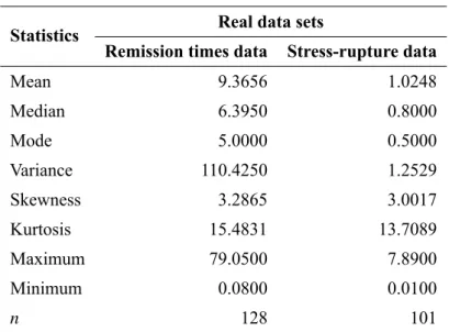
TABLE IV Descriptive statistics.

Statistics Real data sets

Remission times data Stress-rupture data

Mean 9.3656 1.0248

Median 6.3950 0.8000

Mode 5.0000 0.5000

Variance 110.4250 1.2529

Skewness 3.2865 3.0017

Kurtosis 15.4831 13.7089

Maximum 79.0500 7.8900

Minimum 0.0800 0.0100

n 128 101

wherea>0,b>0,c>0andβ >0. Another model is the beta Weibull (BW) distribution, whose pdf is

given by

g(t) = α λB(a,b)

_t

λ

α−1

[1−exp{−(t/λ)α}]a−1exp{−b(t/λ)α},

wherea>0,b>0,α>0andλ >0. The Beta-Fréchet (BFr) distribution, whose pdf is given by

g(t) = λ σ B(a,b)t

−(λ+1)_expaσ t

λ

1−exp

aσ t

λb−1

,

wherea>0,b>0,λ >0andσ >0. We also consider the Marshall-Olkin Nadarajah-Haghighi (MONH)

model, whose pdf is given by

g(t) =α β λ (1+λt)

α−1_{exp{1−(1+λt)}α_}

[1−(β−1)exp{1−(1+λt)α_}]2,

whereα>0,β >0andλ>0. The EW distribution, whose pdf is given by

g(t) =α β λtα−1exp(−λtα) [1−exp(−λtα)]β−1, t>0,

whereα>0andβ>0are shape parameters andλ>0is a scale parameter. This distribution is quite flexible

because its hrf presents the classic five forms (constant, decreasing, increasing, upside-down bathtub and bathtub-shaped). The Weibull model is a special case of the EW model whenβ=1.

The ENH distribution can also have the same shapes for the hrf and therefore can be an interesting alternative to the EW distribution in modeling positive data. The ENH density is given by (6) whenγ=1.

Further, forγ=β =1, we have as a special model the NH distribution given by (2). We also consider the

PGW model, whose pdf is given in (4), which arises from the EPGW model whenβ =1.

Xie et al. (2002) proposed a modified Weibull (MW) density given by

g(t) =λ βt α

1−β

exp

_t

α

β

+λ α

1−exp

n_t

α

oβ

0.0 0.2 0.4 0.6 0.8 1.0

0.0

0.2

0.4

0.6

0.8

1.0

i/n

T(i/n)

(a)

0 10 20 30 40 50

0.04

0.06

0.08

0.10

0.12

0.14

x1

h(x)

(b) Figure 4 -The TTT plot(a)and EPGW hrf for the remission times data(b).

whereλ >0,β >0andα >0. Forα =1, it becomes the Chen distribution (Chen 2000). The MW and

Chen distributions can have increasing or bathtub-shaped failure rate. An extension of the Weibull model proposed by Bebbington et al. (2007) has pdf given by

g(t) =

α+β t2

exp

αt−β

t

exp

−exp

αt−β

t

, t>0,

whereα>0 andβ >0. We shall use the same terminology by Lemonte (2013) for this distribution, i.e.,

denote the flexible Weibull (FW) density. The FW model can have increasing or modified bathtub-shaped failure rate.

We use the simulated-annealing method for maximizing the log-likelihood function of the models in the two applications. The MLEs and goodness-of-fit statistics are evaluated using theAdequacyModelscript in

Rsoftware. Tables V and VI list the MLEs and the corresponding standard errors (SEs) in parentheses of the unknown parameters for the fitted models to remission times data (first data set) and stress-rupture failure times (second data set), respectively.

In applications there is qualitative information about the failure rate shape, which can help for selecting some models. Thus, a device called the total time on test (TTT) plot is useful. The TTT plot is obtained by plotting

Tr n

=

" _r

∑

yi:n+ (n−r)yr:n

# , _n

∑

yi:n,

againstr/n, wherer=1, . . . ,nandyi:n(i=1, . . . ,n)are the order statistics of the sample.

TABLE V

The MLEs of the model parameters for the remission times data and the corresponding SEs in parentheses.

Distributions Estimates

EPGW(α,β,λ,γ) 0.2076 0.4062 0.0047 3.1008

(0.0347) (0.0547) (0.0025) (0.2866) Kw-W(a,b,c,β) 3.8071 1.7364 0.5144 0.2904

(1.3951) (0.8486) (0.1157) (0.1435) BW(a,b,α,λ) 6.4498 8.3256 0.3909 25.4616

(2.7464) (4.3776) (0.0859) (18.7415) BFr(a,b,λ,σ) 4.1513 8.8050 0.3087 8.8088

(1.4516) (2.6397) (0.0460) (4.0961) PGW(α,λ,γ) 0.4253 0.1364 1.5564

(0.0996) (0.0359) (0.2212) MONH(λ,α,β) 1.1844 0.5025 6.3566

(0.5670) (0.0480) (3.1274) EW(β,λ,γ) 0.4854 0.5421 3.9736

(0.1821) (0.0619) (1.0804) MW(α,β,λ ) 0.0030 0.1979 2.2188

(0.0009) (0.0063) (0.6607) ENH(α,β,λ) 0.6003 0.4002 1.7880

(0.0841) (0.1614) (0.3419)

NH(α,λ) 0.9134 0.1236

(0.1475) (0.0344) Chen(β,λ) 0.1106 0.3538

(0.0152) (0.0123) Weibull(α,λ) 9.5470 1.0490

(0.8499) (0.0676)

FW(α,β) 0.0325 2.1553

(0.0026) (0.2490)

Chen and Balakrishnan (1995) constructed the corrected Cramér-von Mises and Anderson-Darling statistics. We adopt these statistics, where we have a random samplex1, . . . ,xn with empirical distribution

functionFn(x), and require to test if the sample comes from a special distribution. The Cramér-von Mises

(W∗) and Anderson-Darling (A∗) statistics are given by

W∗ =

n

Z +∞

−∞ {Fn(x)−F(x;

b

θn)}2dF(x;θbn)

1+0.5 n

= W2

1+0.5

n

TABLE VI

The MLEs of the model parameters for the stress-rupture data and the corresponding SEs in parentheses.

Distributions Estimates

EPGW(α,β,λ,γ) 0.1349 0.1022 0.0415 6.6681

(0.0171) (0.0104) (0.0154) (0.0136) Kw-W(a,b,c,β) 0.7029 0.2175 1.0118 4.3625

(0.1620) (0.1038) (0.0027) (2.1072) BW(a,b,α,λ) 0.7482 0.2305 1.1275 0.3245

(0.1608) (0.0338) (0.0858) (0.0856) BFr(a,b,λ,σ) 0.3984 5.0048 0.4208 9.1684)

(0.1702) (1.4399) (0.0534) (4.3072) PGW(α,λ,γ) 1.2659 0.7182 0.8696

(0.4483) (0.3485) (0.1039) MONH(λ,α,β) 0.0146 17.7252 0.2122

(0.0067) (7.7187) (0.0618) EW(β,λ,γ) 0.8488 1.0419 0.8171

(0.2981) (0.2511) (0.3157) MW(α,β,λ ) 0.0027 0.2259 7.0190

(0.0008) (0.0076) (1.5244) ENH(α,β,λ) 1.0732 0.7762 0.8426

(0.2760) (0.3582) (0.1238)

NH(α,λ) 0.8898 1.1810

(0.1853) (0.4270) Chen(β,λ) 0.5410 0.5303

(0.0585) (0.0321) Weibull(α,λ) 0.9919 0.9259

(0.1121) (0.0726)

FW(α,β) 0.3287 0.0838

(0.0246) (0.0133)

and

A∗ =

(

n

Z +∞

−∞

{Fn(x)−F(x;θbn)}2

{F(x;θbn)[1−F(x;θbn)]}

dF(x;θbn) )

1+0.75 n +

2.25

n2

= A2

1+0.75 n +

2.25

n2

,

respectively, whereFn(x)is the empirical distribution function,F(x; ˆθn)is the postulated distribution

0.0 0.2 0.4 0.6 0.8 1.0

0.0

0.2

0.4

0.6

0.8

1.0

i/n

T(i/n)

(a)

0 1 2 3 4 5 6 7

0.6

0.8

1.0

1.2

x

h(x)

(b) Figure 5 -The TTT plot(a)and EPGW hrf for the stress-rupture failure data(b).

andF(x; ˆθn). Thus, the lower are these statistics, we have more evidence thatF(x; ˆθn)generates the sample.

The details to evaluate the statisticsW∗andA∗are given by Chen and Balakrishnan (1995).

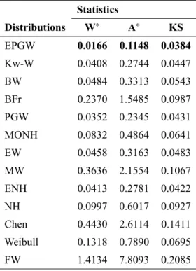
TheW∗,A∗and Kolmogorov-Smirnov (KS) statistics for these models are given in Tables VII and VIII

for both data sets. We emphasize that the EPGW model fits the remission times and stress-rupture failure data better than the other models according to these statistics. They indicate that the EPGW distribution yields the best fits in both applications.

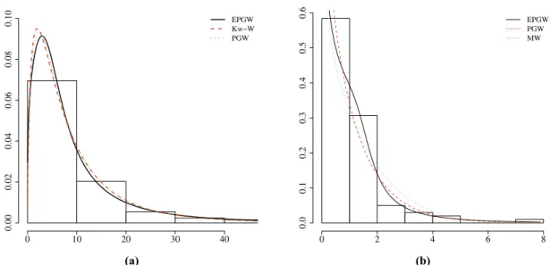
More information is provided by the histogram of the data and some fitted density functions for both data sets given in Figure 6. Clearly, in both applications, the new distribution provides a closer fit to the histogram than the other competitive models. The fitted cdfs of these models are also displayed in Figure 7. Finally, we can conclude in the two situations that the EPGW distribution is quite competitive to other well-known and widely used distributions such as the Kw-W, EW and Weibull models.

14 - CONCLUSIONS

TABLE VII

Goodness-of-fit statistics for the models fitted to the remission times data.

Statistics

Distributions W∗ _A∗ _KS

EPGW 0.0166 0.1148 0.0384

Kw-W 0.0408 0.2744 0.0447

BW 0.0484 0.3313 0.0543

BFr 0.2370 1.5485 0.0987

PGW 0.0352 0.2345 0.0431

MONH 0.0832 0.4864 0.0641

EW 0.0458 0.3163 0.0483

MW 0.3636 2.1554 0.1067

ENH 0.0413 0.2781 0.0422

NH 0.0997 0.6017 0.0927

Chen 0.4430 2.6114 0.1411

Weibull 0.1318 0.7890 0.0695

FW 1.4134 7.8093 0.2085

TABLE VIII

Goodness-of-fit statistics for the models fitted to the stress-rupture data.

Statistics

Distributions W∗ _A∗ _KS

EPGW 0.0722 0.4672 0.0699

Kw-W 0.1400 0.8478 0.1017

BW 0.2753 1.5190 0.1005

BFr 0.7116 3.8276 0.1914

PGW 0.1730 0.9930 0.0833

MONH 1.1054 5.9604 0.3068

EW 0.1686 0.9736 0.0875

MW 0.0980 0.7596 0.1292

ENH 0.1670 0.9667 0.0837

NH 0.2053 1.1434 0.0819

Chen 0.1207 0.8756 0.0973

Weibull 0.1987 1.1115 0.0900

0 10 20 30 40

0.00

0.02

0.04

0.06

0.08

0.10 EPGW

Kw−W

PGW

(a)

0 2 4 6 8

0.0

0.1

0.2

0.3

0.4

0.5

0.6

EPGW PGW MW

(b)

Figure 6 -Histogram and estimated densities of the(a)EPGW, Kw-W and PGW models for the remission times data;(b)EPGW, PGW and MW models for the stress-rupture data.

0 20 40 60 80

0.0

0.2

0.4

0.6

0.8

1.0

x

F

(x)

EPGW Kw−W PGW

(a)

0 2 4 6 8

0.0

0.2

0.4

0.6

0.8

1.0

x

F

(x)

EPGW PGW MW

(b)

Figure 7 -Estimated and empirical cdfs for(a)EPGW, Kw-W and PGW models for the remission times data;(b)EPGW, PGW and MW models for the stress-rupture data.

REFERENCES

ANDREWS DF AND HERZBERG AM. 1985. Data: A Collection of Problems from Many Fields for the Student and Research Worker. New York: Springer Series in Statistics, 442 p.

BAGDONAVICIUS V AND NIKULIN M. 2002. Accelerated life models: modeling and statistical analysis. Boca Raton: Chapman and Hall/CRC, 360 p.

BEBBINGTON M, LAI CD AND ZITIKIS R. 2007. A flexible Weibull extension. Reliab Eng and Syst Safe 92: 719-726. CHEN G AND BALAKRISHNAN N. 1995. A general purpose approximate goodness-of-fit test. J Qual Technol 27: 154-161. CHEN Z. 2000. A new two-parameter lifetime distribution with bathtub shape or increasing failure rate function. Stat Probabil Lett

49: 155-161.

DIMITRAKOPOULOU T, ADAMIDIS K AND LOUKAS S. 2007. A lifetime distribution with an upside-down bathtub-shaped hazard function. IEEE T Reliab 121: 308-311.

EUGENE N, LEE C AND FAMOYE F. 2002. Beta-normal distribution and its applications. Commun Stat Theory Methods 31: 497-512.

GOMES O, COMBES C AND DUSSAUCHOY A. 2008. Parameter estimation of the generalized gamma distribution. Math Comput Simul 79: 963-995.

GRAHAM RL. 1994. Concrete mathematics: a foundation for computer science, 2nd_{ed., Boston: Addison-Wesley, 672 p.} GUPTA R, GUPTA P AND GUPTA R. 1998. Modeling failure time data by Lehman alternatives. Commun Stat Theory Methods

27: 887-904.

LAI CD. 2013. Constructions and applications of lifetime distributions. Appl Stoch Model Bus 29: 127-140. LEE E AND WANG J. 2003. Statistical Methods for Survival Data Analysis, 3rd_{ed., New York: Wiley, 534 p.}

LEMONTE AJ. 2013. A new exponential-type distribution with constant, decreasing, increasing, upside-down bathtub and bathtub-shaped failure rate function. Comput Stat Data An 62: 149-170.

MACGILLIVRAY H. 1986. Skewness and asymmetry: measures and orderings. Ann Stat 14: 994-1011.

NADARAJAH S, BAKOUCH H AND TAHMASBI R. 2011. A generalized Lindley distribution. Sankhya Ser B 73: 331-359. NADARAJAH S AND HAGHIGHI F. 2011. An extension of the exponential distribution. Statistics 45: 543-558.

NIKULIN M AND HAGHIGHI F. 2006. A chi-squared test for the generalized power Weibull family for the head-and-neck cancer censored data. J Math Sci 133: 1333-1341.

NIKULIN M AND HAGHIGHI F. 2009. On the power generalized Weibull family. Metron 67: 75-86.

TAHIR MH AND NADARAJAH S. 2015. Parameter induction in continuous univariate distributions: Well-established G families. An Acad Bras Cienc 87: 539-568.