Allocation of SCR by lines of business and RORAC optimization

UNIVERSIDADE DE LISBOA

I

S

E

G

M

ASTER

’

S

F

INAL

W

ORK

I

R

A

LLOCATION OF

SCR

BY

L

INES OF

B

USINESS

AND

RORAC

O

PTIMIZATION

B

D

P

MS

C

A

CTUARIAL

S

CIENCE

ii

UNIVERSIDADE DE LISBOA

I

S

E

G

M

ASTER

’

S

F

INAL

W

ORK

I

R

A

LLOCATION OF

SCR

BY

L

INES OF

B

USINESS

AND

RORAC

O

PTIMIZATION

B

D

P

SUPERVISED BY:

WALTHER ADOLF HERMANN NEUHAUS

ANA MANUELA P.SILVA FERREIRA

MS

C

A

CTUARIAL

S

CIENCE

1

OCTOBER-2016

A

Nowadays topics that are related with the new insurance supervisory regime, Solvency II, have been becoming increasingly important. This is due to the fact that insurance companies must follow this regime from January 1, 2016. This project focuses on the study of risk-based capital, SCR, which is calculated using the standard formula proposed by EIOPA. However, the formula calculates the SCR of the insurance company as a whole. Which creates a problem for purposes like identification of risk concentration, perception of sensitivity of the risk and the optimization of the portfolio. Therefore, it is necessary to have an idea of risk-based capital that is necessary to allocate to each of the lines of business (sub-portfolios). Which is a very challenging task since there is some partial correlation between the risks (from where the diversification effect appears) in different levels of the formula, this effect needs to be incorporated in the allocated capital in such a way that the sum of the allocated capital would be the company’s global SCR. The main goal of this project is to allocate the SCR between sub-portfolios (lines of business), using a method developed by Dirk Tasche which is based on Euler’s formula, and show how this allocation could be used in the optimization of the portfolio in such a way that the maximization of the RORAC of the company is reached.

For the academic purposes this study should contribute to the better understanding of the standard formula and the SCR, show some properties that SCR follows, how it is possible to do a fair allocation of SCR between lines of business and show a practical example of this method applied to a non-life insurance company.

For business purposes this investigation will show a practical step-by-step demonstration of the application of the model. In my opinion this project should support the analysis of decisions that are made by the management of the company.

By applying this model to a real data of a non-life insurance, we obtained a very interesting result: some LoBs that at first sight seem to be profitable, show high volatility, and we conclude that they do not fulfill the risk appetite of the company.

Keywords

Solvency II; SCR; Standard Formula; RORAC; capital allocation; Euler’s allocation principle; diversification; risk appetite; optimization; profitability.

2

OCTOBER-2016

R

Atualmente, temas ligados ao novo regime Solvência II têm vindo a assumir uma importância crescente, muito devido ao facto de se exigir às seguradoras que, a partir do dia 1 de janeiro de 2016, sigam este novo regime de solvência.

Esta investigação incide sobre o estudo do capital em risco, SCR, que é calculado através da Fórmula Padrão proposta pela EIOPA. Esta fórmula calcula o SCR da seguradora como um todo, mas se se pretender fazer uma análise da concentração do risco, uma análise da sensibilidade ao risco ou da otimização do portfolio, é necessário alocar o SCR por cada uma das linhas de negócio (sub-portfolios) presentes na seguradora. Tal tarefa pode não se revelar fácil pois existe uma correlação parcial dos riscos (do qual resulta o efeito da diversificação), em diferentes níveis da fórmula, que tem que ser incorporada na alocação feita de modo a que a soma do capital alocado seja o SCR global.

O objetivo do trabalho é alocar o SCR por linhas de negócio através de um método, desenvolvido por Dirk Tasche que se baseia na fórmula de Euler, e mostrar como esta alocação poderá ser usada na otimização do portfolio da seguradora de modo a que a maximização do RORAC seja atingida.

A nível académico este estudo irá contribuir para uma melhor compreensão da Fórmula Padrão e do SCR, mostrar algumas propriedades do SCR, mostrar como é possível a sua alocação por linhas de negócio e a aplicar todo este modelo a um caso prático.

A nível empresarial, esta investigação irá mostrar um modelo de alocação do SCR aplicado à Formula Padrão juntamente com um exemplo da sua aplicação. Penso que este trabalho será interessante para atuários, gestores de risco ou mesmo administradores, que poderão aplicá-lo nas suas decisões de gestão da empresa.

Ao aplicar o modelo a uma seguradora não vida, foram obtidos resultados bastante interessantes pois linhas de negócio que a primeira vista parecem lucrativas, mostraram--se bastante voláteis, o que faz com que o retorno não é compensado pelo risco, ou seja é ultrapassado o limite da volatilidade proposto pela empresa (apetite ao risco da empresa).

3

OCTOBER-2016

A

I would like to thank the insurance company’s actuarial team who proposed me this topic for my Master’s final work and guided me during the internship period. I also wanted to recognize the indispensable support that was given to me by my professor from ISEG Walther Neuhaus and the author of the paper from which I based my investigation Dr. Ivan Granito.

4

C

1 A Brief Introduction to Solvency II ... 9

1.1 Risk ... 9

1.2 Risk Management ... 9

1.2.1 Risk management in Non-Life insurance ... 11

1.2.2 Lines of Business (LoBs) in Non-Life insurance ... 11

2 Solvency II ... 12

2.1 Why Solvency II was Implemented ... 12

2.2 Goals of Solvency II ... 12

2.3 Three Pillars of Solvency II ... 13

2.3.1 Quantitative Requirements ... 13

2.3.2 Technical provisions ... 14

2.3.2.1 Best Estimate (BE) ... 14

2.3.2.2 Risk Margin (RM) ... 15

2.3.3 Minimum Capital Requirement (MCR) ... 15

2.3.4 Solvency Capital Requirement (SCR) ... 15

2.3.5 Definition of Non-Life insurance risks ... 16

2.4 Solvency II Standard Formula (SF) ... 19

2.5 Capital Allocation ... 20

2.6 Return on Risk-Adjusted Capital (RORAC) ... 20

2.7 Optimization Strategy ... 20

3 Mathematical Framework ... 20

5

OCTOBER-2016

3.2 Risk Measure ... 21

3.3 Defining the Allocation Problem ... 22

4 Euler’s Allocation Method... 23

4.1 RORAC compatibility ... 24

4.2 Defining contribution of each sub-portfolio ... 24

4.3 Euler allocation and sub-additive risk measures ... 25

5 Applying Euler’s method ... 26

5.1 General basis ... 26

5.2 Allocation Procedure ... 27

6 RORAC optimization problem ... 29

6.1 Company’s Risk Appetite ... 29

6.2 Lines of business evaluation ... 30

6.3 RORAC maximization strategies ... 31

7 Application to a non-life insurance ... 32

7.1 Application of Euler method for Underwriting Risk ... 32

7.2 Possible simplifications for allocating other risk module by LoB ... 34

7.2.1 Market risk allocation by LoB ... 35

7.2.2 Counterparty Default risk allocation by LoB ... 36

7.3 Allocated BSCR by LoB ... 36

7.4 Allocated SCR Operational and Adjustments by LoB ... 37

7.5 Allocated SCR ... 38

7.6 Return per unit of Risk ... 38

7.7 Portfolio Optimization ... 40

8 Conclusion ... 42

References... 44

Appendix ... 46

6

OCTOBER-2016

B Data ... 48

C Non-Life Premium and Reserve allocation for LoB 4 ... 49

C1 Allocation of risk capital between risk modules ... 49

C2 Allocation Ratio ... 49

C3 Allocation of risk capital for Motor Vehicle Liability ... 50

7

OCTOBER-2016

L

F

Figure 1: The risk management cycle steps according to Vaughan (2008)... 10

Figure 2: Solvency II Balance Sheet displaying assets (left) and liabilities (right). ... 13

Figure 3: Technical Provision of liability side of Solvency II Balance Sheet. ... 14

Figure 4: Hierarchy of Risks. ... 17

Figure 5: Return per unit of risk. ... 39

L

T

Table 2: Allocation of risk capital between risk modules. ... 32

Table 3: First level allocation ratio. ... 33

Table 4: Capital required for 𝑗-th risk submodule gross of the diversification. ... 33

Table 5: Allocation of risk capital between 𝑗-th mirco risk (net of the diversification). 33 Table 6: Allocated BSCR by LoB of each sub-portfolios of Health risk module. ... 34

Table 7: Allocated BSCR by LoB of each sub-portfolio of Non-Life risk module. ... 34

Table 8: Allocated Risk Capital of Market Risk by LoB Net of Diversification. ... 35

Table 9: Allocated Risk Capital of Default risk modules by LoB Net of Diversification. ... 36

Table 10: Allocated BSCR by LoB. ... 37

Table 11: Allocated 𝐴𝑑𝑗 and 𝑆𝐶𝑅 Operational by LoB. ... 37

Table 12: Allocated SCR by LoB. ... 38

Table B1: Correlation between risk modules. ... 48

Table B2: Correlation between Micro Non-Life risks... 48

Table B3: Correlation between Non-Life LoB. ... 48

Table B4: Correlation between Micro Non-Life risks... 48

Table B5: Correlation between Health LoB.. ... 48

8

OCTOBER-2016

I

After the introduction of Solvency II it is crucial that all financial institutions measure the risk in their portfolio in terms of economical capital. However, measuring it for the total portfolio does not give any information to risk managers for purposes like identification of risk concentration, risk sensitivity or portfolio optimization. That is the reason why it is important to decompose the total portfolio into sub-portfolios.

There is a lot of research being done about different methodologies for capital allocation. In this project, I will present the Euler’s allocation principle, developed by Dirk Tasche and described in the paper “Capital allocation and risk appetite under Solvency II

framework” (by Ivan Granito and Paolo de Angelis), and its application to a small

Portuguese non-life insurance company. After a proper allocation is done, we will see that Euler’s compatibility with the Return on Risk-Adjusted Capital (RORAC) will allow us to evaluate which Lines of Business (LoBs) create value to the company. Also, by using the same approach, I will show that it is possible to optimize the company’s portfolio.

This final project was proposed by the non-life Portuguese insurance company that offered me a four-month internship. During this time, I had the opportunity not only to develop this investigation, but also to work with experienced actuaries and analyze the real problems that insurance companies are facing today. This experience will surely strengthen my knowledge and will allow me to face the next steps in my professional career.

The internship started with the presentation of techniques and procedures that actuaries use to calculate their provisions. I was shown methods that used bootstrap and chain ladder modeling which gave me the opportunity to implement my knowledge of Loss Reserving.

My first task was the calculation of the SCR of the company by applying standard formula, where I had the chance to read carefully the delegated act offered by EIOPA and construct the Standard formula in excel using the data of the company. This information allowed me to go further, explore SCR and understand how it is possible to allocate SCR by LoB, since Standard Formula allows only the calculation of SCR of the whole company.

9

OCTOBER-2016

When proceeding with the risk capital allocation I perceived that I would face a problem related to the allocation of the diversification effect by LoB. I noticed that it is not possible to analyze the capital requirements of each LoB by themselves, since it is also important to incorporate the diversification effects, which will lower this capital.

In this paper, the Euler’s allocation method is proposed, since it ensures RORAC compatibility and allows practical application. This approach, applied to Standard Formula, was presented by Dr. Granito and Prof. Angelis.

1

A

B

I

S

II

1.1 Risk

In this section we introduce the common elements and definitions of this topic.

Definition 1 (Risk). It is a situation where the probability distribution of a variable is

known, but the actual value of the variable is not.

~ Is it good or bad?

Insurance companies offer products to cover many different risks. The decision whether to cover a risk or not must be taken after a proper analysis of the risk (for example look at the frequency and severity of the risk) and the market price, in order to see if it will be profitable. These decisions, made by the risk managers, will determine whether risks are good or not.

1.2 Risk Management

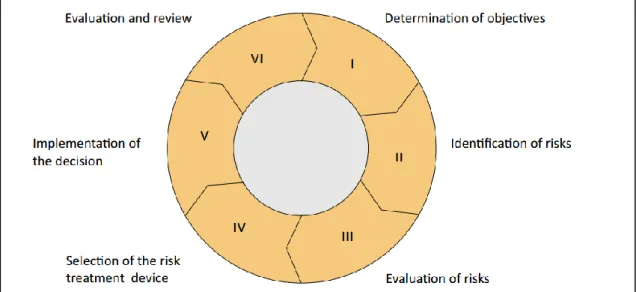
Analyzing the risk and whether it will be profitable to the company or not, and measuring it, is a very complex process. Therefore, it is necessary to perform a proper risk management and it consists in the following steps:

10

OCTOBER-2016

Figure 1: The risk management cycle steps according to Vaughan (2008).

A good risk management enhances the chance of the company to reach its goals ensuring that it does not go bankrupt. This is done by preventing the acceptance of “bad risks”1 that have high probability of generating financial losses to the company. Poor risk management can lead to severe consequences not only to the company or to all individuals related to it, but also to economic instability through a domino effect. The 2008 crisis is an excellent example.

After the financial disaster, EU implemented new regulations in the insurance and banking industry, therefore a more intense preparation to this new regime, Solvency II, had started.

The Solvency II is a “Directive in European Union law that codifies and harmonizes the

EU insurance regulation. Primarily, this concerns the amount of capital that EU insurance companies must hold to reduce the risk of insolvency.”. The main goal of this

regime is the protection of policyholders and beneficiaries, implying that insurance companies must guarantee their solvency.

11

OCTOBER-2016

1.2.1 Risk management in Non-Life insurance

Risk management of the insurance company must fulfill specific requirements written in the Solvency II regime, which follow a risk-based approach. In non-life insurance, claim severities are unknown, so it is very important to do a proper risk management and evaluate the risks involved as well as their concentration in the portfolio. One possible way of lowering the implicit risk is to share it with the reinsurance companies.

However, by spreading the risk, the insurance company loses a share of the business since the expected profitability is also shared. Therefore, it´s important that the risk manager elaborates a proper contract with the reinsurer in a way that allows the reduction of the risk (by splitting it with the reinsurer) and at the same time earn profit from it.

1.2.2 Lines of Business (LoBs) in Non-Life insurance

Insurance companies sell innumerous products that cover all sorts of risks. These can lead to profit or loss, consequently, it is up to the company study these risks and decide whether to cover them or not. For the organizational purposes, EIOPA formed twelve groups, each one of them is composed by homogeneous risks2_{. These groups are called}

lines of businesses (LoBs).

Since insurance companies have the obligations with the policyholders that buy their products, LoBs segment the liability side of the insurance company’s balance sheet, these LoBs are3:

 Non-life groups: (1) motor vehicle liability; (2) other motor; (3) marine aviation and transport (MAT); (4) Fire; (5) Third party liability; (6) Credit; (7) Legal expenses; (8) Assistance; (9) Miscellaneous.

 Health groups: (10) Medical Expenses; (11) Income Protection; (12) Workers' Compensation.

Each one of them will produce positive or negative results to the company, therefore, to analyze the profitability of the whole company, we should evaluate and build strategies

2_{Products that have similar characteristics.}

12

OCTOBER-2016

to each LoB separately. Note that by treating them disjointedly we need to have in mind that there is a relation between sales of different products in different LoBs. Therefore, sometimes it is not possible nor desirable to sell LoBs separately, knowing this, we conclude that strategies of portfolio optimization should take into account this relation.

2

S

II

Solvency II is a new regulatory plan for the European insurance sector, that was implemented on January 1, 2016. It considers more effective risk management approached and ensures that, theoretically speaking, ruin of the company occurs no more often than once in every 200 years (probability of default in one-year period is 0.5%). Therefore, the company needs to ensure to have necessary amounts of risk-based capital, the SCR, to guarantee that the probability of ruin will not exceed 0.5%. From this we can see that the capital that the company is required to hold on the risks it is facing, specifically, the riskier the insurance’s business the more precautions it needs to take, consequently more capital is required. From investor’s perspective, the capital is a scarce resource so to attract more investments insurance companies want to demonstrate their profitability, by showing their sufficiently high return per unit of capital invested and low volatility.

2.1 Why Solvency II was Implemented

We have seen recently a huge Financial Crisis starting from 2007/2008, that was the consequence of the burst of a “financial bubble” at international level. Through a “snowball effect” it contaminated the entire banking system, which led to liquidity problems and forced banks to sell assets. With a huge supply in the market the asset’s prices fell drastically and since we are living in an Era of Globalization most of developed countries were affected. In order to prevent these types of crisis, the EU decided to be more demanding from the banking and insurance business4_.

2.2 Goals of Solvency II

1) Policyholder protection: this is the main goal of Solvency II, that ensures the policyholder’s protection, so that the consumers would have confidence on insurance

13

OCTOBER-2016

products. This will eventually increase the demand of the insurance’s products which in turn favors the grow of the insurance market.

2) Better supervision: supervisors have very important roles on monitoring the insurance’s risk profile, risk management and administration strategies.

3) EU Integration: Insurers in all EU countries should obey similar rules.

2.3 Three Pillars of Solvency II

To achieve these goals Solvency II proposed following three Pillars:

i) Pillar I (quantitative requirements): EU expects from the insurances calculations

of technical provisions, capital requirements (SCR and MCR), investments and calculation of own funds. These outputs will form the major items of the balance sheet of the insurance company;

ii) Pillar II (qualitative requirements): effective risk management, Own Risk

Solvency Assessment (ORSA) and supervisory review process;

iii) Pillar III (market discipline and transparency): detailed public disclosure,

improvement of market discipline by facilitating comparisons and regulatory reporting requirements.

2.3.1 Quantitative Requirements

Figure 2: Solvency II Balance Sheet displaying assets (left) and liabilities (right).

Source: The Underwriting assumptions in the standard formula for the Solvency Capital Requirement calculation (EIOPA)

14

OCTOBER-2016

The main goal for the valuation of assets and liabilities “set out in Article 75 of Directive 2009/138/EC” is to have an economic and market-consistent approach.

1. Assets should be valued at the amount for which they could be transferred to knowledgeable willing parties.

2. Liabilities should be valued at the amount for which they could be settled between knowledgeable willing parties.

2.3.2 Technical provisions

Solvency II requires to set up Technical Provisions (TP), which correspond to the current amount that the undertakings would have to pay if they would transfer their (re)insurance obligations today to another undertaking. TP are calculated as market value and the formula is:

𝑇𝑃 = 𝐵𝐸 + 𝑅𝑀 (1)

Figure 3: Technical Provision of liability side of Solvency II Balance Sheet.

Source: The Underwriting assumptions in the standard formula for the Solvency Capital Requirement calculation (EIOPA)

2.3.2.1

Best Estimate (BE)

Best Estimate (BE) is the probability weighted average of future gross cash-flows taking into account the time value of the money. In other words, through the use of actuarial approaches, it is necessary to calculate future cash-flows and after discount them at an interest rate, given by EIOPA. The projection horizon used in the calculation of BE should cover the full lifetime of all in-flows and out-flows required to settle the obligations related to the existing contracts on the date of the valuation.

15

OCTOBER-2016

2.3.2.2

Risk Margin (RM)

Risk Margin is the amount over BE that an independent third party (reference undertaking) would ask in order to take over the liabilities. This amount ensures that the value estimated for technical provisions is sufficient for other (re)insurer to take the obligations of the first one. It is calculated through Cost of Capital methodology, that is, by determining the cost of providing an amount of eligible own funds equal to SCR, which is necessary to support the obligations during their lifetime and it is calculated as following:

I. Calculate BE technical provision in each point (future year) during all lifetime; II. Estimate the appropriate corresponding SCR at each future year;

III. Multiply by cost-of-capital factor; IV. Apply the discounting factor to the sum.

𝐶𝑂𝐶𝑀 = 𝐶𝑜𝐶 ∗ ∑ 𝑆𝐶𝑅𝑅𝑈 (𝑡)

(1+𝑟𝑡+1)𝑡+1

𝑡≥0 , (2)

where, 𝐶𝑂𝐶𝑀 is the risk margin for the whole business, 𝐶𝑜𝐶 is the cost-of-capital rate (set at 6%), 𝑆𝐶𝑅𝑅𝑈(𝑡) is the SCR as calculated for the reference undertaking at the 𝑡-th

year and 𝑟_𝑡 is the risk-free rate for maturity 𝑡.

2.3.3 Minimum Capital Requirement (MCR)

The MCR is the minimum level of capital that is necessary in order for (re)insurance undertakings to be allowed to continue their operations. If the amount of eligible own funds falls below that level the policyholders and beneficiaries are exposed to an unacceptable level of risk. For this reason, the supervisors must analyze these problematic (re)insurers more carefully. If those undertakings are unable to re-establish the amount of eligible basic own funds at the MCR level within a short period of time the supervisors should take withdraw the authorization of (re)insurance business. Calculation of MCR should be simple and easy to understand such that the audit could easily verify them.

2.3.4 Solvency Capital Requirement (SCR)

16

OCTOBER-2016

The SCR is the amount of capital that ensures that the probability of default in one-year period should be no more than 0.5% and it is calculated by the usage of one of the following procedures:

i) Internal Model: is created by the (re)insurance company, using their own parameters and methodologies in order to calculate the SCR. This model should be approved by the supervisors and it should explain more precisely the situation of the company where it is being used than the Standard Formula. However, this procedure is very complex and expensive, so not every company can afford it;

ii) Using Standard Formula with company’s own parameters, instead of those given by EIOPA, which result from approximation by all EU insurance companies;

iii) Using Standard Formula as it is written by EIOPA;

In this paper, I will use the third method, that is the Standard Formula with the parameters given in delegated act by EIOPA but the same procedures could be applied to those companies that use the second approach.

2.3.5 Definition of Non-Life insurance risks

When actuaries calculate predictions, it is always necessary to remember that no model is perfect, so there are always deviations from the predictions that were made. Even if they use the best model possible there are still some unpredictable anomalies that can occur.

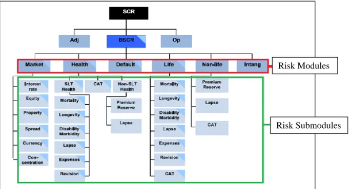
There are enormous variety of risks that an insurance company is facing that could put it in insolvent position, since we cannot incorporate all risks in the model, EIOPA decided to select those that are the most important and use them in the calculation of the SCR as the figure below shows:

17

OCTOBER-2016

Figure 4: Risks involved in SCR calculation

Figure 4: Hierarchy of Risks.

Source: EIOPA Delegated Act

The figure above shows the combination of risks that are involved in the calculation of SCR. When observing Figure 4, by doing the general-specific analysis, we notice that we can divide risks in different levels: BSCR (that results from the combination of risk modules), risk modules (that results from the combination of risk submodules), risk

submodules (that result from the combination of lines of business (LoBs)) and LoBs.

Since the analysis is done to a non-life insurance company the only risk modules that required capital by Standard Formula are: Non-life, Health, Market and Default. Giving a brief explanation of each5:

~ For Non-Life:

 Premium Risk: the risk that the premiums will not be sufficient to cover the future liabilities and the expenses that have resulted from claims;

 Reserve Risk: the risk that the liabilities that come from past claims will turn out to be higher than expected;

 CAT: the risk of the catastrophe, which means if single or series of correlated events will cause huge deviation in actual claims from the total expected claims;

5 _{Assuming that there is no intangible risk.}

Risk Modules

18

OCTOBER-2016

 Lapse Risk: the risk that the insurance company have higher than expected premature contract termination;

~ For Health:

 Health Similar to Life (SLT) divided into:

o Longevity Risk: the risk that person live longer than expected, this will put more weight on the pension provision thus higher costs;

o Disability Morbidity: the risk that more people will have higher disability pension than expected;

o Expense Risk: the risk of possible increase in expenses;

o Revision Risk: the risk of unexpected revision of the claims, which can lead to higher liabilities (this is applied to the annuities).

o Mortality Risk: “is the risk of loss, or of adverse change in the value of re(insurance) liabilities, resulting from changes in level, trend, or volatility of mortality rates.”

o Lapse Risk: “is the risk of loss, or of adverse change in the value of re(insurance) liabilities, resulting from changes in the level or volatility of the rates of policy lapses, terminations, renewals and surrenders.”

 CAT: the risk of the catastrophe, that is, if single or series of correlated events will cause huge deviation in actual claims from the total expected claims (mass accident, concentration scenario and pandemic scenario).

 Health Non-Similar-to-Life (Non-SLT) divided into:

o Premium Risk: the risk that the premiums will not be sufficient to cover the future liabilities and the expenses that have resulted from claims; o Reserve Risk: the risk that the liabilities that come from past claims will

turn out to be higher than expected;

o Lapse Risk: the risk that the insurance company have higher than expected premature contract termination;

19

OCTOBER-2016

~ For Market (definitions given by EIOPA):

 Interest Rate Risk: “the sensitivity of the values of assets, liabilities and financial instruments to changes in the term structure of interest rates, or in the volatility of interest rates”;

 Equity Risk: “the sensitivity of the values of assets, liabilities and financial instruments to changes in the level or in the volatility of market prices of equities”;  Property Risk: “the sensitivity of the values of assets, liabilities and financial instruments to changes in the level or in the volatility of market prices of real estate”;

 Spread Risk: “the sensitivity of the values of assets, liabilities and financial instruments to changes in the level or volatility of credit spreads over the risk-free interest rate term structure”;

 Currency Risk: “the sensitivity of the values of assets, liabilities and financial instruments to changes in the level or in the volatility of currency exchange rates”.

~ For Default:

 This module reflects possible losses due to unexpected default of the counterparties and debtors of undertakings over the forthcoming twelve months. If we want to calculate SCR by LoB, as you can see, it is not straightforward since the risks presented above are correlated with each other in different levels, and because of that, a diversification effect is produced each time we go from one level to the next.

2.4 Solvency II Standard Formula (SF)

The insurance company, that is being analyzed, uses the SF (with parameters given by EIOPA) to calculate its SCR. As it was seen previously, this was one of three methods to calculate SCR and it is not perfect. SF aims to capture the risks that most undertakings are exposed to. However, it might not cover all risks that a specific undertaking is exposed to, also the parameters that are used in standard formula are an average at EU level and do not reflect the reality of a specific insurance.

For this reasons the standard formula might not reflect the true risk profile for a specific insurance and, consequently, the level of own funds it needs. Yet, creating internal models

20

OCTOBER-2016

can be very expensive and not all the insurances can afford it, this is why SF is being used by a lot of insurance companies around the EU.

2.5 Capital Allocation

In order to analyze the business strategy of the company it is necessary to evaluate the profitability and the risk that each LoB produce. As it was previously shown, the SF calculates SCR of the company as a whole. Thus, to do a proper analysis it is important to allocate this risk-based capital to each LoB, such that the sum of allocated SCRs gives us the total SCR of the company. In other words, the allocation must be done in such a way that the diversification effect would be incorporated in the allocated capital.

2.6 Return on Risk-Adjusted Capital (RORAC)

This is very popular measure that is used in the financial analysis every time it is necessary to evaluate risky investments. It is based on the ratio of earnings divided by the risk-based capital, from which it is possible to determine the percentage of return that a particular investment obtained weighted by the capital that was invested in order to get this return.

2.7 Optimization Strategy

After a proper allocation is done, it is possible to analyze the RORAC not only of a present situation, but also compare it with other RORAC obtained by different strategies, that the management board of the company propose, in such a way that the one that maximizes the company’s RORAC is chosen.

3

M

F

It was seen that the risks that are involved in the calculation of SCR are not perfectly correlated with each other, in different levels of SF, from where the diversification effect appears. To allocate SCR by LoBs a proper mathematical approach should be applied. There are several approaches that can be used to allocate risk capital, the method that is being used in this thesis is based on Euler’s principle.

21

OCTOBER-2016

3.1 General Basis

Let’s consider an insurance company that has a portfolio that is composed by 𝑛-homogeneous sub-portfolios, each of those sub-portfolios can bring profit or loss to the global result of the company. Define a set of random variables 𝑋_𝑖 (𝑖 =1, …, 𝑛) , where 𝑋_𝑖 represents the risk of the 𝑖 − 𝑡ℎ sub-portfolio. It is clear that the portfolio-wide risk that the company is facing is:

𝑋 = ∑𝑛𝑖=1𝑋𝑖 (3)

To do a proper analysis of the risk of an insurance company, it is necessary to apply a risk measure that calculates capital that is necessary to be kept in the company, so that the risk would be acceptable.

3.2 Risk Measure

Let π be the risk measure that quantifies the level of risk, then π(X) is the real number that represents the capital that is necessary to cover risk X. As we saw previously, 𝑆𝐶𝑅(𝑋) is a measure of the risk that calculates the risk capital that is required by the regulators for the amount of the risk X.

𝑆𝐶𝑅(𝑋) = π(X) (4)

It is clear that the riskier the (re)insurance strategy (higher X) the more capital is required by the authority (higher the π(X)), but this relation is not linear because of the correlation between risks. In order to proceed to the allocation problem a desirable risk measure must satisfy the following properties:

Definition 2 (Coherent Risk Measure). A risk measure 𝜋 is considered coherent if it

satisfies the following properties:

i) Subadditivity: For all bounded random variables 𝑋 and 𝑌 we have:

𝜋(𝑋 + 𝑌) ≤ 𝜋(𝑋) + 𝜋(𝑌) (5)

ii) Monotonicity: For all bounded random variables, such that 𝑋 ≤ 𝑌 we have:

22

OCTOBER-2016

iii) Positive Homogeneity: Consider 𝜆 ≥ 0 and bounded random variable 𝑋 we

have:

𝜋(𝑋𝜆) = 𝜆𝜋(𝑋) (7)

iv) Translation invariance: for a fixed return α Є ℝ, bounded random variable 𝑋

and riskless investment whose price today is 1 and price at some point in the future is 𝐵

𝜋(𝑋 + 𝛼𝐵) = 𝜋(𝑋) − 𝛼 (8)

Remark 1. From above, property: (i) shows that risk-based capital of holding two risky

sub-portfolios at same time is smaller or equal than when we are holding them separately, this happens due the imperfect correlation between 𝑋 and Y; (ii) shows that if the loss of sub-portfolio X is, in all scenarios, less or equal than the loss Y, then X is less risky than Y , thus needs less capital; (iii) explains that the risk of a portfolio is proportional to its size, and (iv) tells us that if we add some riskless investment to the portfolio it will reduce the risk of the company by the return of that riskless investment.

3.3 Defining the Allocation Problem

If the firm’s overall risk capital (π(𝑋)) is smaller than the sum of all sub-portfolios stand-alone risks (∑𝑛𝑖=1π(𝑋𝑖)), we have a diversification effect. This motivates the usage of an

allocation principle that can separate the insurance company’s overall risk capital among sub-portfolios in such a way that this effect is allocated to the sub-portfolios.

Definition 3 (Allocation Principle). Given a risk measure 𝜋, an allocation principle is

defined as a mapping 𝛱: 𝐴→ℝ𝑛_{, that maps each allocation problem into a unique}

allocation. Let 𝑋 denote portfolio-wide risk, we have:

𝛱(𝐴) = 𝛱 ( 𝜋(𝑋1) ⋮ 𝜋(𝑋𝑛)) = ( 𝜋(𝑋_1|𝑋) ⋮ 𝜋(𝑋_𝑛|𝑋) ) (9)

where, 𝜋(𝑋_𝑖|𝑋) is the allocated risk capital for sub-portfolio 𝑖, such that the risk

contributions 𝜋(𝑋1|𝑋) … 𝜋(𝑋𝑛|𝑋) to portfolio-wide risk 𝜋(𝑋) satisfies the full allocation

23

OCTOBER-2016

Definition 4 (Allocated Risk Capital). This form of capital for a sub-portfolio 𝑖 is the

capital adjusted for a maximum probable loss that can occur and it is based on the estimation of the future earnings distribution.

Each of the allocated risk capitals incorporates the diversification benefits that came from imperfect risk correlation. Note that the allocated risk capital does not coincide with real capital invested to fund a portfolio, but it can be used to virtually express each sub-portfolio’s contribution to the risk of the whole (re)insurance company and can be the point of reference to know the profitability of each sub-portfolio.

Definition 5 (Coherent Allocation)6_{. An allocation 𝐾}

𝑖,such that: 𝑖 ∈ 𝑁, is coherent if

satisfies the following properties:

i) Full allocation: ∑𝑖∈𝑁𝐾𝑖 = 𝜋( ∑𝑖∈𝑁𝑋𝑖)

ii) No undercut ∀ 𝑀 ⊆ 𝑁, ∑_𝑖∈𝑀𝐾_𝑖 ≤ 𝜋(∑_𝑖∈𝑀𝑋_𝑖)

iii) Symmetry: If by joining any subset 𝑀 ⊆ 𝑁\ {𝑖, 𝑗}, portfolios 𝑖 and 𝑗 both make the

same contribution to the risk capital, then 𝐾𝑖 = 𝐾𝑗.

iv) Riskless allocation for a riskless deterministic portfolio 𝐿 with fixed return 𝛼 we

have: 𝐾_𝑛 = 𝜋(𝛼𝐿) = −𝛼.

Remark 2. As we saw previously (i) ensures that the sum of the allocated capital by

sub-portfolios would be the same as the risk capital of the whole portfolio. (ii) ensures that there is no subset M of the set portfolios which is cheaper for every single portfolio in M; (iii) guarantees that a portfolio’s allocation depends only on its contribution to risk within the (re)insurance company, and (iv) says that riskless investments will lower the capital at risk of a portfolio, since the returns of that investment are guaranteed with zero risk.

4

E

’

A

M

The Euler’s allocation principle can be applied to any risk measure that is homogeneous of degree 1 and is continuously differentiable7. This is one of the most common allocation methods with very useful properties that allow us to study the performance of the portfolio.

6 _{These properties were given in Michael Denault’s work (1999)} 7 _{Defined in Annex D}

24

OCTOBER-2016

4.1 RORAC compatibility

RORAC is a very popular measure that is being used in financial analysis that evaluates the return based on risk-based capital and it is calculated the following way:

𝐸(𝑅𝑂𝑅𝐴𝐶) = 𝐸(𝐸𝑎𝑟𝑛𝑖𝑛𝑔𝑠)

𝐶𝑎𝑝𝑖𝑡𝑎𝑙 𝑎𝑡 𝑟𝑖𝑠𝑘 (10)

Definition 6 (Return on Risk Adjusted Capital). Let the expected one-year income of

the 𝑖 − 𝑡ℎ-sub-portfolio be 𝜇𝑖, such that ∑𝑛𝑖=1𝜇𝑖 is the expected one-year income of the

whole company, then the total portfolio Return on Risk Adjusted Capital is given by:

𝐸(𝑅𝑂𝑅𝐴𝐶(𝑋)) =∑𝑛𝑖=1𝜇𝑖

𝜋(𝑋) . (11)

If conditioned, then the 𝑖-sub-portfolio Return on Risk Adjusted Capital is:

𝐸(𝑅𝑂𝑅𝐴𝐶(𝑋𝑖|𝑋)) = 𝜇𝑖

𝜋(𝑋𝑖|𝑋) (12)

Definition 7 (RORAC Compatibility)8_{. Let 𝑋 denote portfolio-wide profit/loss as in}

Definition 3, then we say that risk contributions 𝜋(𝑋𝑖|𝑋) are 𝑅𝑂𝑅𝐴𝐶 compatible if there

are some 𝜖𝑖 > 0 such that:

𝑅𝑂𝑅𝐴𝐶(𝑋_𝑖|𝑋) > 𝑅𝑂𝑅𝐴𝐶(𝑋) ⇒ 𝑅𝑂𝑅𝐴𝐶(𝑋 + ℎ𝑋_𝑖) > 𝑅𝑂𝑅𝐴𝐶(𝑋), (13)

for all 0 < ℎ < 𝜖_𝑖.

In other words, if there is 𝑖 − 𝑡ℎ sub-portfolio that has by its own a bigger RORAC than the RORAC of the portfolio where it is placed, than if we increase the amount invested in this sub-portfolio, the RORAC of the whole portfolio will be forced to go up.

4.2 Defining contribution of each sub-portfolio

As we saw previously, the SF calculates the risk capital of the whole company, consequently to build an optimal risk strategy it is necessary to answer the following question: How much does each sub-portfolio 𝑖 contribute to risk-based capital of the

8 _{To have a better understanding I invite the reader to look at Dirk Tasche paper (1999): “Capital Allocation}

25

OCTOBER-2016

whole company 𝜋(𝑋)? From now on we denote 𝜋(𝑋_𝑖|𝑋) as the risk contribution net of

diversification effect of 𝑖-sub-portfolio, such that π(𝑋) = ∑𝑛_𝑖=1π(𝑋_𝑖|X).

Proposition 1. Let 𝜋 be a risk measure that is homogeneous of degree 1 and is

continuously differentiable9. If there are risk contributions 𝜋(𝑋₁|𝑋) … 𝜋(𝑋𝑛|𝑋) that are

RORAC compatible (see Definition 7), they can be determined as: 𝜋𝐸𝑢𝑙𝑒𝑟(𝑋𝑖|𝑋) = 𝜋(𝑋𝑖) ∗

𝜕𝜋(𝑋)

𝜕𝜋(𝑋𝑖) (14)

where, 𝜋𝐸𝑢𝑙𝑒𝑟(𝑋𝑖|𝑋) is a uniquely allocated risk capital for the sub-portfolio 𝑖 where 𝑖 =

1, … , 𝑛 and 𝑛 is the number of lines of business of an insurance company.

Remark 3. If 𝜋 is a homogeneous of degree 1 and continuously differentiable risk measure, then using Euler allocation from equation (14), we produce Euler’s contributions of each sub-portfolio. These contributions satisfy both properties stated in Definitions 3 and 7.

4.3 Euler allocation and sub-additive risk measures

From the Definition 2, risk measures that fulfill the sub-additive property are rewarded with portfolio diversification, therefore Euler’s allocation principle is a very popular allocation method, since it considers the diversification effect10 and the calculations that are involved are simple to understand.

Remark 4. Let π be a risk measure that is sub-additive, continuously differentiable and homogeneous of degree 1. After applying the allocation method given in formula (14) it is easy to obtain the following result:

𝜋_{𝐸𝑢𝑙𝑒𝑟}(𝑋_𝑖|𝑋) ≤ 𝜋(𝑋_𝑖) (15)

This relation means that if we calculate Euler contributions of a risk measure, that is homogeneous and sub-additive, we conclude that the contribution to risk capital of a single sub-portfolio will never exceed the risk capital of the same sub-portfolio stand alone. This makes sense because of the benefit of the diversification effect.

9 _{Defined in Annex D}

26

OCTOBER-2016

5

E

’

From Section 2, it was clear that the SF calculates the SCR for a company as a whole. In this calculation, many risks are involved and they are all correlated with each other at different levels as we will see.

5.1 General basis

We present some new notation that will be used in the following Sections. The SF has 𝑛 risk modules, each one is represented with letter 𝑖 = 1, … , 𝑛, every 𝑖-th risk modules is composed by 𝑚_𝑖 risk submodules.

Let 𝐿_𝑖𝑗 be the random variable that represents losses that can occur over the one-year period related with 𝑖-th risk modules and 𝑗-th risk submodule, and let 𝑌𝑖𝑗 = 𝐿𝑖𝑗 − 𝐸(𝐿𝑖𝑗)

be the random variable that represents the unexpected losses. The total risk that the company is facing 𝑌 can be calculated as:

𝑌 = ∑𝑛𝑖=1∑𝑚_𝑗=1𝑖 𝑌𝑖𝑗, (16)

where, 𝑌_𝑖 = ∑𝑚𝑖𝑌_𝑖𝑗

𝑗 such that

 ∑ 𝑌𝑚𝑖 _𝑖𝑗

𝑗 ∶ is the sum of risk submodules that exist in 𝑖-th risk modules;

 ∑𝑛𝑖=1∑𝑚_𝑗=1𝑖 𝑌𝑖𝑗: is the sum of 𝑛 risk modules that exist in the whole portfolio.

As previously shown, if we want to transform the risk into risk capital, a proper risk measure should be applied. When EIOPA introduced Solvency II regime it proposed the Standard Formula (SF) which will allow us to calculate the risk-based capital (SCR). In this Section I will present the most important formulas of the SF and explain them:

𝑆𝐶𝑅 = 𝐵𝑆𝐶𝑅 + 𝐴𝑑𝑗 + 𝑆𝐶𝑅𝑂𝑃, (17)

where, 𝐵𝑆𝐶𝑅 is the Basic Solvency Capital Requirement, 𝐴𝑑𝑗 is adjustment for the loss absorbing effect of technical provisions and deferred taxes and 𝑆𝐶𝑅𝑂𝑃 is the capital

requirement for operational risk..

We assume that the BSCR is the only one that depends on the aggregation scheme allowing us to use Euler’s method, 𝐴𝑑𝑗 𝑎𝑛𝑑 𝑆𝐶𝑅_𝑂𝑃 depends on considerations that are made by the company.

27

OCTOBER-2016

𝐵𝑆𝐶𝑅 = √∑_𝑖𝑤𝜌_𝑖𝑤∙ 𝑆𝐶𝑅_𝑖 ∙ 𝑆𝐶𝑅_𝑤+ 𝑆𝐶𝑅_{𝑖𝑛𝑡𝑎𝑛𝑔𝑖𝑏𝑙𝑒} (18) where, 𝜌𝑖𝑤 is the correlation between risk modules available in delegated act, 𝑆𝐶𝑅𝑖 ∙

𝑆𝐶𝑅_𝑤 are solvency capital requirement for risk modules and 𝑆𝐶𝑅_{𝑖𝑛𝑡𝑎𝑛𝑔𝑖𝑏𝑙𝑒} is the capital requirement for intangible asset (it is assumed that there is no intangible asset). To calculate the capital required for the 𝑖-th risk modules (𝑆𝐶𝑅_𝑖), a similar approach is applied:

𝑆𝐶𝑅𝑖 = √∑ ∑𝑚𝑧𝑖𝜌𝑗𝑧∙ 𝑆𝐶𝑅𝑗∙ 𝑆𝐶𝑅𝑧 𝑚𝑖

𝑗 (19)

where, 𝑆𝐶𝑅_𝑖 is the solvency capital requirement for 𝑖-th risk modules, 𝜌_𝑗𝑧 is the correlation between 𝑗-th and 𝑧-th risk submodule, respectively, and 𝑆𝐶𝑅_𝑗, 𝑆𝐶𝑅_𝑧 are solvency capital requirement for risk submodule 11.

The choice of a risk measure within the overall Solvency system was not an easy task, two measures were presented Value-at-Risk (VaR) and Tail-Value-at-Risk (TVaR). After the analysis of pros and cons, it was stated that in practical work one of the most significant disadvantages using TVaR is the complexity and the scarcity of data about the tails of the distributions applicable to life or non-life insurance companies.12 Therefore, to provide a good fit to the majority of insurance companies the SCR is calibrated using VaR of the basic own funds of an (re)insurance undertaking subject to a confidence level of 99.5% over one-year period.13

𝑆𝐶𝑅𝑖𝑗 = 𝑉𝑎𝑅99.5%(𝑌𝑖𝑗)

5.2 Allocation Procedure

In the previous Section, we saw the definition of coherent risk measures, that is the necessary condition for the allocation procedure. In order for the SCR to be coherent,

11 _{Note that each of the SCR for risk submodule is calculated according to SF.}

12 _{This could lead to an increase in modelling error and would make it difficult to calibrate any system}

designed to produce TVaR consistent with SF estimates, this problem can only be solved when more data is available about the company’s tail and it is only available in big insurance companies.

28

OCTOBER-2016

since it is calibrated using VaR risk measure, the risk is assumed to be normally distributed.14

Proposition 2. We start the allocation with BSCR, that is our final risk capital that

comprises all the diversification effects according to the SF, to each of risk modules in such a way the condition 𝐵𝑆𝐶𝑅 = ∑𝑛_𝑖=1𝑆𝐶𝑅(𝑌_𝑖|𝑌) must hold.15 From the Proposition D.1 (Annex D) we obtain:

𝑆𝐶𝑅(𝑌_𝑖|𝑌) = 𝑆𝐶𝑅𝑖∗

∑𝑛𝑤=1𝑆𝐶𝑅𝑤∗𝜌𝑖 𝑤

𝑆𝐶𝑅𝑌 , (20)

where:

 𝑆𝐶𝑅(𝑌_𝑖|𝑌) : is the allocated risk capital to 𝑖 − 𝑡ℎ risk modules;

 𝜌_{𝑖 𝑤} : is the correlation between the risk modules i and w, given by EIOPA;

 𝑆𝐶𝑅𝑖 : is the risk capital of 𝑖 − 𝑡ℎ risk module gross of diversification effect;

 𝑆𝐶𝑅_𝑌 : is the risk capital for the total company’s risk 𝑌, that is our BSCR.

Proposition 3. To realize the diversification effect that have occurred to 𝑖-th risk module,

due to risk modules correlation, I will introduce the variable Allocation Ratio (𝐴𝑅_𝑖): 𝐴𝑅_𝑖 =𝑆𝐶𝑅(𝑌𝑖|𝑌)

𝑆𝐶𝑅𝑖 =

∑𝑛𝑤=1𝑆𝐶𝑅𝑤∗𝜌𝑖 𝑤

𝑆𝐶𝑅𝑌 (21)

In case of an insurance company the correlation between any different part of risks16, given by EIOPA, is always less than one, which means that insurance companies are favored when they are diversifying their portfolio. This causes 𝐴𝑅 < 1, that comes from

sub-additive property, as we shall see in the practical example.

Proposition 4. After an allocation of BSCR by macro-risks has been done, we can

proceed to the allocation of our BSCR by each risk submodule, ensuring that the condition

𝐵𝑆𝐶𝑅 = ∑ ∑𝑚𝑖 𝑆𝐶𝑅_𝑖𝑗 𝑗=1 𝑛 𝑖=1 hold. 𝑆𝐶𝑅(𝑌_𝑖𝑗|𝑌, 𝑌_𝑖) = 𝑆𝐶𝑅_𝑖𝑗∗∑ 𝑆𝐶𝑅𝑖 𝑧 𝑚𝑖 𝑧=1 ∗𝜌𝑖𝑗,𝑖𝑧 𝑆𝐶𝑅𝑖 ∗ 𝐴𝑅𝑖 (22) where:

 𝑆𝐶𝑅(𝑌_𝑖𝑗|𝑌, 𝑌_𝑖) : is the allocated capital for 𝑗 − 𝑡ℎ risk submodule that is situated

in 𝑖 − 𝑡ℎ risk module;

14 _{If it is not the case, then VaR does not satisfy the sub-additivity property, as it was shown by Artzner}

(1999)

15_{Note that each time I say allocated risk capital it is net of diversification effect.} 16 _{This is valid because the intangible risk is excluded from investigation.}

29

OCTOBER-2016

 𝑆𝐶𝑅_𝑖𝑗 : is the risk capital of 𝑗 − 𝑡ℎ risk submodule that is situated in 𝑖 − 𝑡ℎ risk

module gross of diversification effect;

 𝜌_{𝑖𝑗,𝑖𝑧} : is the correlation between risk submodules 𝑖 𝑎𝑛𝑑 𝑧 situated in 𝑖 − 𝑡ℎ risk

module;

 𝑆𝐶𝑅𝑖 : is the risk capital of 𝑖 − 𝑡ℎ risk module gross of diversification effect;

 𝐴𝑅_𝑖 : is the allocation ratio for 𝑖 − 𝑡ℎ risk module.

Remark 5: This allocation is a general-specific process, where we start from the top level

of our formula, in our case the BSCR, and we allocated it by more specific levels of risks, by risk modules (20) and by risk submodules (22), ensuring always that the sum of allocated capital would get our BSCR. The idea is to continue our allocation until we reach the lines of business, using similar methodology as in formula (22).

6

RORAC

It is clear that Solvency II regime forces insurance companies to implement risk based approaches, therefore, to build an optimal strategy, managers should, not only analyze the result of a particular LoB, but also evaluate the cost in terms of risk capital that this LoB requires and also the volatility that comes with it. After a fair allocation of the risk capital between lines of businesses, we can analyze the company’s performance through the RORAC measure. It was proved that Euler’s allocated contributions follow the full

allocation property in sense of Definition 3 and are RORAC compatible by satisfying the

condition given in Definition 7, where the second will allow us to proceed to the optimization problem.

6.1 Company’s Risk Appetite

Risk appetite can be defined as “The amount and type of risk that an organization is

willing to take in order to meet their strategic objectives”17_{. This means that similar} organizations that have comparable portfolios can have very different risk appetites depending on their sector, location and objectives. In most cases Risk appetite is established by the top managers of the company. After its settlement, it should be always considered when any decision is made about the strategic plan of the company. From the study made, we can conclude that the most important strategies that non-life insurance

30

OCTOBER-2016

companies can have are based on the optimization of the underwriting and reinsurance policies, since the quantity of risk-based capital necessary depends, mostly, on them18_.

Therefore, when dealing with the optimization of the RORAC it is better to focus on setting optimal reinsurance and underwriting policies.

6.2 Lines of business evaluation

The underwriting of insurance lines of business (LoB) is considered as a risky activity, since we cannot guarantee their returns. Consequently, if we want to compare them we cannot only analyze their returns, it is also important to look at the risk involved in those activities.

In previous Sections we saw that the allocation method applies satisfies both: Definition 3 (Full allocation) and Definition 7 (RORAC compatibility), that are essential for further investigation. With the purpose of comparing the LoB return in terms of risk capital we will use the following formulas:

𝐸(𝑅𝑂𝑅𝐴𝐶𝑟) = 𝐸(𝐸𝑎𝑟𝑛𝑖𝑛𝑔𝑠𝑟) 𝐴𝑙𝑙𝑜𝑐𝑎𝑡𝑒𝑑 𝑆𝐶𝑅𝑟 , 𝜎(RORACr) = 𝜎(𝐸𝑎𝑟𝑛𝑖𝑛𝑔𝑠𝑟) 𝐴𝑙𝑙𝑜𝑐𝑎𝑡𝑒𝑑 𝑆𝐶𝑅𝑟 (23) where:

 𝐸(𝑅𝑂𝑅𝐴𝐶_𝑟) is expected value of the RORAC of 𝑟 − 𝑡ℎ LoB;

 𝐴𝑙𝑙𝑜𝑐𝑎𝑡𝑒𝑑 𝑆𝐶𝑅_𝑟 is the allocated risk capital of 𝑟 − 𝑡ℎ LoB obtained by Euler’s method;

 𝐸(𝐸𝑎𝑟𝑛𝑖𝑛𝑔𝑠_𝑟) = 𝑃𝑠_𝑟∗ (1 − E(𝐶𝑅_𝑟)) with 𝑃𝑠_𝑟 being the estimate of the premiums to be earned by the insurance or reinsurance undertaking during the following 12 months of 𝑟-th LoB and E(𝐶𝑅_𝑟) defined as the expected value of the combined ratio of 𝑟-th LoB.

 𝜎(𝐸𝑎𝑟𝑛𝑖𝑛𝑔𝑠_𝑟) = 𝑃𝑠_𝑟∗ σ(𝐶𝑅_𝑟) with σ(𝐶𝑅_𝑟) defined as the standard deviation of the combined ratio of 𝑟-th LoB.

Note that since we do not have a proper distribution for the combined ratio, it is necessary to apply a model which will allow us to calculate E(𝐶𝑅_𝑟) and σ(𝐶𝑅_𝑟). Before going any

18 _{Note that the capital-at-risk of market risk also plays a huge role, and has a high weight in SCR, but it is}

31

OCTOBER-2016

further, I advise the reader first to understand the model of the combined ratio that is presented in Annex A.

6.3 RORAC maximization strategies

In non-life insurance, the risk that usually requires the most risk capital is the underwriting risk, therefore the purpose of the following Section is to show how it is possible to analyze different strategies, for example by changing the variables like reinsurance agreement, business volume or the premiums that the company charges, to determine the strategy that maximizes the company’s RORAC.

As previously shown, each company has different risk appetite, therefore it is necessary to build the optimization problem in most general form possible, so that this procedure can be adapted to all non-life companies. The difference of the risk appetite in different companies can be seen in the proposal of different limits. Therefore, similar companies with same resources but with different risk appetites could have different strategies to optimize their portfolio.

For the evaluation of the different strategies, that were set by the managers, we suggest the following optimization problem that derived from a mean-variance model:

𝑀𝑎𝑥𝑖𝑚𝑖𝑧𝑒: 𝐸(𝑅𝑂𝑅𝐴𝐶) 𝑎 < 𝑆𝐶𝑅 < 𝑏,

𝜈𝑖 < 𝑃𝑆𝑖 < 𝜀𝑖,

𝐶𝑉_𝑖 < 𝛼, where:

 𝐸(𝑅𝑂𝑅𝐴𝐶) : is the Expected value for the RORAC of the company;

 𝑆𝐶𝑅 : is the Solvency Capital Required for the whole company and it should be between values 𝑎 and 𝑏 (limits);

 𝑃_𝑆𝑖: is the future premium of 𝑖 − 𝑡ℎ LoB and it should be between values 𝜈_𝑖 and 𝜀_𝑖 (limits for 𝑖 − 𝑡ℎ LoB);

 𝐶𝑉_𝑖 : is the coefficient of variation of 𝑖 − 𝑡ℎ LoB;

 𝛼 : could be considered as the the risk appetite of the company. Subject to:

32

OCTOBER-2016

The main goal of this problem is to always maximize the global E(RORAC) of the company and considering the risk appetite of the company. We can impose limits for global SCR, business volume for each LoB (𝑃_𝑆𝑖) and coefficient of variation of each LoB, in such a way that the company’s risk appetite will not be exceeded. From the management point of view there are not so many strategies that a company is willing to take so analyzing each of them one by one is not that time consuming.

7

A

-

In this Section I will put into practice to a real non-life insurance the methodologies that were presented in last sections. This will allow us to witness the likely difficulties that can arise with the theoretical framework applied to real data and the possible solutions and simplifications that were used to address them.

7.1 Application of Euler method for Underwriting Risk

Consider a non-life insurance that calculates its SCR using Standard Formula with the parameters given by EIOPA and where the following results were obtained:

Table 1: Capital Requirement for 𝑖-th risk module gross of the diversification.

From Table 1 it is easy to see that the sum of the capital requirement of each risk module is different from the BSCR because of the risk correlation consequently, to allocate the risk capital we can apply the formula (20) where the correlation between risk modules is given in Annex B and the following risk module allocation is obtained:

Table 2: Allocation of risk capital between risk modules.

BSCR 27,786,074 Macro Risk Market 7,573,591 Default 558,862 Health 9,756,580 Non Life 21,954,662

Table 1: Capital requirement for i-th macro risk gross of the diversification

Macro Risk SCR(Yi|Y)

Market 4,263,266

Default 319,168

Health 4,139,739

Non Life 19,063,900

Total 27,786,074

33

OCTOBER-2016

Table 2 shows that after incorporating the diversification effect, which lowers the risk capital, it is possible to sum the allocated risk module capital and the result will be company’s BSCR. From the Formula (21) we have:

Table 3: First level allocation ratio.

Remark 6. It is clear that since the risk measure fulfills the sub-additive property the

following inequality will always occur: 𝐴𝑅 ≤ 1.

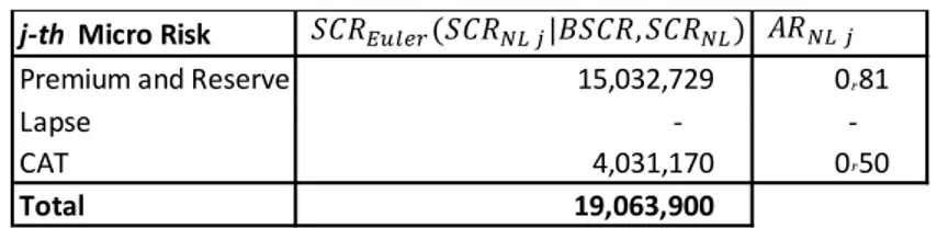
Formula (22) will allow us to continue allocate the risk capital by risk submodules, e.g. in Non-Life we have:

-First we calculate the capital gross of diversification effect:

Table 4: Capital required for 𝑗-th risk submodule gross of the diversification.

-Now, applying formula (22), where the correlation between risk submodule is given in Annex B.2:

Table 5: Allocation of risk capital between 𝑗-th mirco risk (net of the diversification).

Remark 7: The sum of NL risk submodule capital allocation given in Table 5 match with

allocated non-life risk capital specified in Table 2 thus we can conclude that the full

allocation property given in Definition 3 is fulfilled. By implementing the same Macro Risk

Market 0.56 Default 0.57 Health 0.42 Non Life 0.87 Table 3: 1st level allocation ratio

Micro Risk

Premium and Reserve 18,516,265 Lapse

-CAT 8,043,084

Table 4: Capital required for j-th micro risk gross of the diversification 𝑆𝐶𝑅_𝑖𝑗

j-th Micro Risk

Premium and Reserve 15,032,729 0.81 Lapse - -CAT 4,031,170 0.50

Total 19,063,900

Table 5: Allocation of risk capital between j-th micro risk (net of the diversification) 𝑆𝐶𝑅𝐸𝑢𝑙𝑒𝑟(𝑆𝐶𝑅𝑁 𝑗|𝐵𝑆𝐶𝑅, 𝑆𝐶𝑅𝑁 ) 𝐴𝑅𝑁 𝑗

34

OCTOBER-2016

methodology in different levels of Standard Formula to underwriting risk (NL and Health), we will allocate the risk capital by LoB (simplest form that SF allow)19_:

-For Health we have:

Table 6: Allocated BSCR by LoB each sub-portfolios of Health risk module.

-For Non-Life we have:

Table 7: Allocated BSCR by LoB each sub-portfolio of Non-Life risk module.

The last column of above tables also shows that the full allocation property given in Definition 3 is fulfilled.

7.2 Possible simplifications for allocating other risk

module by LoB

In Non-Life insurance company, the risk group that require the most risk capital is the Underwriting (Health and Non-Life risk modules), as we saw previously to allocate it by LoB we could use the Euler’s method and we obtain the results given in Table 7 and Table 6. From Figure 4 we can see that there are also Default and Market risk modules that also needed to be allocated by LoB.

19_{Note that to understand better the allocation process, analyze the Annex C that shows the example of a complete calculation of the} allocation process for NL risk module

LoB Health SLT Health CAT Health Non SLT

1. Medical Expenses - - 4,916 4,916 2. Income Proteccion - 629,568 1,300,614 1,930,182 3. Workers' Compensation 547,503 - 1,657,137 2,204,641

Total 547,503 629,568 2,962,667 4,139,739

Table 6: Allocated BSCR by LoB each sub-portfolios of Health Macro risk

LoB NL Premium and Reserve NL Lapse NL CAT

4.Motor vehicle liability 11,572,959 - 35,052 11,608,011 5.Other motor 908,151 - - 908,151 6.MAT 33,521 - - 33,521 7.Fire 1,885,959 - 3,991,993 5,877,952 8.Third party liability 548,662 - 4,126 552,788 9.Credit - - - -10.Legal expenses 17,849 - - 17,849 11.Assistance 64,612 - - 64,612 12.Miscellaneous 1,016 - - 1,016

Total 15,032,729 - 4,031,170 19,063,900

Table 7: Allocated BSCR by LoB each sub-portfolios of Non-life Macro risk

35

OCTOBER-2016

Table 2 shows the risk-based capital net of diversification effect, but for risk modules, to allocate the risk capital that covers these risk modules by LoB we need to use some simplifications. I will present some possible simplifications that can be used.

7.2.1 Market risk allocation by LoB

For the LoB Workers’ Compensation, there is an obligation to associate assets with responsibilities, in such a way that there would be sufficient assets to cover the liabilities. The (re)insurer’s main goal is to guarantee that the investments made have the average duration adjusted to the liabilities, this will allow, from an economic point of view, the reduction of the interest rate risk.

Having that in mind, the approach that was used for the allocation of the SCR Market was the following:

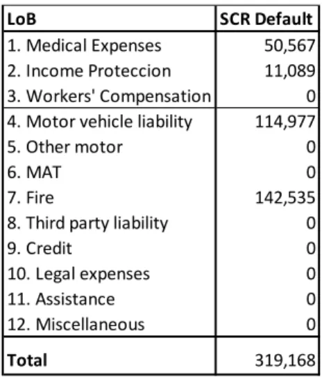
For LoB Workers’ Compensation, since there is a direct connection between LoB and the assets, it was chosen the ones that represent that LoB. For the rest, it was used the following simplification:

1st. In each LoB we sum the Best Estimate (BE) for Premiums and Reserves; 2nd. We calculate how much percentage each LoB’s BE sum represent in of total of

BE of the company;

3rd. We multiplied this percentage by SCR Market Net of Diversification, that is

given in Table 2. The following result is obtained:

Table 8: Allocated Risk Capital of Market Risk by LoB Net of Diversification.

LoB SCR Market

1. Medical Expenses 4,664 2. Income Proteccion 237,209 3. Workers' Compensation 1,546,977 4. Motor vehicle liability 1,911,893 5. Other motor 158,606

6. MAT 1,596

7. Fire 332,608

8. Third party liability 68,869

9. Credit 0

10. Legal expenses 17

11. Assistance 800

12. Miscellaneous 26

Total 4,263,266