SOIL THERMAL DIFFUSIVITY ESTIMATED FROM DATA OF
SOIL TEMPERATURE AND SINGLE SOIL COMPONENT
PROPERTIES
(1)Quirijn de Jong van Lier(2) & Angelica Durigon(2)
SUMMARY
Under field conditions, thermal diffusivity can be estimated from soil temperature data but also from the properties of soil components together with their spatial organization. We aimed to determine soil thermal diffusivity from half-hourly temperature measurements in a Rhodic Kanhapludalf, using three calculation procedures (the amplitude ratio, phase lag and Seemann procedures), as well as from soil component properties, for a comparison of procedures and methods. To determine thermal conductivity for short wave periods (one day), the phase lag method was more reliable than the amplitude ratio or the Seemann method, especially in deeper layers, where temperature variations are small. The phase lag method resulted in coherent values of thermal diffusivity. The method using properties of single soil components with the values of thermal conductivity for sandstone and kaolinite resulted in thermal diffusivity values of the same order. In the observed water content range (0.26-0.34 m3 m-3), the average thermal
diffusivity was 0.034 m2 d-1 in the top layer (0.05-0.15 m) and 0.027 m2 d-1 in the
subsurface layer (0.15-0.30 m).
Index terms: soil thermal properties, modeling.
RESUMO : DIFUSIVIDADE TÉRMICA DO SOLO ESTIMADA POR
OBSERVAÇÕES DE SUA TEMPERATURA E POR PROPRIEDADES DOS SEUS COMPONENTES
A difusividade térmica do solo sob condições de campo pode ser estimada a partir de dados da sua temperatura, mas pode também ser estimada por meio das propriedades individuais dos seus componentes junto com a sua organização espacial. A difusividade térmica
(1) Received for publication on March 1st, 2012 and approved on November 28, 2012.
(2) Department of Biosystems Engineering, University of São Paulo, Caixa Postal 9. CEP 13418-900 Piracicaba (SP), Brazil.
foi determinada com base em dados de temperatura do solo registrados de meia em meia hora num Nitossolo Vermelho, empregando-se três procedimentos de cálculo (o da razão das amplitudes, da defasagem e do proposto por Seemann), bem como a partir das propriedades individuais dos seus componentes, fazendo-se comparação entre procedimentos e métodos. Para a determinação da difusividade para períodos de onda curtos (um dia), o procedimento da defasagem apresentou-se mais confiável do que o da razão de amplitudes ou o do Seemann, especialmente para a determinação em camadas mais profundas, onde as variações térmicas são pequenas, pois apresentou valores coerentes para a difusividade térmica. O método que utiliza propriedades individuais dos componentes do solo, com os valores da condutividade térmica para arenito e caulinita, resultou em estimativas da difusividade térmica da mesma ordem de grandeza. Ao longo da faixa de teores de água observada, de 0,26-0,34 m3 m-3, o valor médio da difusividade térmica foi de 0,034 m2 d-1 na camada superficial (0,05-0,15 m) e de 0,027 m2 d-1, na camada subsuperficial (0,15-0,30 m).
Termos de indexação: propriedades térmicas do solo, modelagem.
INTRODUCTION
Soil temperature is important for almost all processes in the soil. To mention a few, the temperature affects density, viscosity and surface tension of fluids physically and is therefore indirectly relevant for soil water retention and conductivity. Chemically, it affects the equilibrium and reaction rates, thus influencing the decomposition of organic matter and agrochemicals. Biologically, it impacts the functioning of enzymes and other more complex biological systems, affecting microbial and root growth (Bowen, 1970; Barber et al., 1988; Nagel et al., 2009).
The modeling of soil temperature in time and depth requires knowledge of the soil surface energy balance and of soil thermal properties: conductivity and specific heat capacity, represented together by the soil thermal diffusivity. Thermal diffusivity can be estimated under field conditions from soil temperature data (Carslaw & Jaeger, 1959; Kirkham & Powers, 1972). Theory and experimental considerations to determine soil thermal diffusivity from measured temperatures are clearly exposed by Horton et al. (1983). Corresponding experimental results have been reported by many authors (Adams et al., 1976; Prevedello, 1993; Ramana Rao et al., 2005; Passerat de Silans et al., 2006; Gao et al., 2007)
Alternatively, thermal diffusivity can also be estimated from the properties of single soil components (solids, water and air) together with their spatial organization. Classical contributions to this approach were published by Gemant (1950) and Farouki (1986).
In this study we aimed to determine soil thermal diffusivity from soil temperature data by three calculation procedures, as well as from soil component properties, for a comparison of procedures and methods.
MATERIAL AND METHODS
Theory
Soil thermal diffusivity from spatiotemporal data
The one-dimensional form of Fourier’s Law of thermal conduction describing the heat flux density
q (kJ m-2 d-1) is written as
dx dT
q=-l (1)
with λ (kJ m-1 d-1 K-1) being the thermal conductivity of the medium, T the temperature (in K or °C) and x (m) the distance. Focusing on vertical heat transport in soils qsoil (kJ m-2 d-1), x can be
substituted by depth z (m) and λ is a function of water content θ. Therefore:
( ) dz dT
qsoil=-l q (2)
The heat conservation equation is written as
( )
dz dq dt dT
c soil
-=
q (3)
where t(d) is the time and c(θ) (kJ m-3 K-1) the volume-based specific heat of the soil, function of θ and total porosity α (m3 m-3), according to
c(θ) = cs(1 - α) + cwθ (4) where cs = 1942 kJ m-3 K-1 is an estimate of the heat
capacity of the solid fraction (Farouki, 1986) and
cw = 4186 kJ m-3 K-1 is the heat capacity of the water
fraction. In equation 4, the specific heat of the air fraction was ignored (cair = 1.17 kJ m-3 K-1 at
standard air pressure and T = 298 K). Combination of equations 2 and 3 yields:
( ) ( ) ( )
úû ù êë
é = Û úû ù êë
é =
dz dT D dz
d dt dT dz
dT dz
d dt
dT
with D(θ) (m2 d-1) being the thermal diffusivity, defined as the ratio between thermal conductivity and volume-based specific heat.
The left-hand side of equation 5 is a first-order differential expression in time, whereas the right-hand side is a second-order differential expression in depth. Considering a constant D over depth, equation 5 can be simplified to:
2 2 dz T d D dt dT = (6)
and for many specific settings solutions are available for equation 6 (Carslaw & Jaeger, 1959), most of them in media where c, λ and D do not vary over distance and time.
Considering the surface temperature over a day or a year to vary according to a sine-wave, the first boundary condition to solve equation 6 is:
úû ù êë é + +
=T A tt j
T a 0sin ;z= 0 (7)
where Ta is the average temperature in one cycle, A0 is the surface temperature amplitude, τ is the period (usually one day or one year) and ϕ is a phase constant.
The second boundary condition to be met is
a T t z T z = ¥ ®( , )
lim ; t= 0 (8)
in other words, at great depths the temperature will be constant in time and equal to the average surface temperature. A solution for equation 6 satisfying the boundary conditions (equations 7 and 8) is (Carslaw & Jaeger, 1959; Kirkham & Powers, 1972):
úû ù êë é -÷ ø ö ç è æ -+ = d z t d z A T
T a t
p 2 sin exp
0 ; z= 0 (9)
Parameter d (m) from equation 9 is called the damping depth and defined by
p tD
d= (10)
When the thermal diffusivity D is known, equation 9 can be used to predict temperature behavior in time and depth. The quality of the results is usually good (Wu & Nofziger, 1999). Cichota et al. (2004) discussed limitations of equation 9 and compared its results to those from numerical methods. Solutions for the simultaneous description of two wave periods (e.g. the daily plus annual variation) are discussed in Elias et al. (2004).
Under the assumption of a constant D per time-and space-step, equation 9 can be used to estimate D
from observations of soil temperature in time and depth. There are several mathematically independent ways of doing so (Horton et al., 1983). The first method employs two temperature amplitudes (A1 and A2, K or °C) measured during the same time interval -usually corresponding to one wave period at two depths (z1 and z2). From equation 9 it can be seen that amplitude A as a function of depth z equals
÷ ø ö ç è æ -= d z A z
A( ) 0exp (11)
and by substitution of (A1, z1) and (A2, z2) two equations with two unknowns (A0 and d) are obtained. Solving for d and substituting by equation 10, the following expression for D is obtained:
2
2 1
1 2
ln ÷÷÷
÷ ø ö ç ç ç ç è æ ÷ ø ö ç è æ -= A A z z
D tp (12)
This method will be referred to as the amplitude ratio method. The second method of estimating D uses the phase lag between the sine waves at the two depths. This is most easily achieved by determining the times at which the temperature wave reaches its maximum (or minimum) value at the two depths, tm1 (d) and
tm2 (d). Then, according to equation 9
d z
t
d z
tm1 1 2 m2 2 2
-=
- pt
t p
(13)
which can be solved for d and D to find
2
1 2
1 2
4 úû
ù ê ë é -= m m t t z z
D tp (14)
We will refer to this method as the phase lag method.
A third method was proposed by Seemann (1979) and quoted (with modifications) by Horton et al. (1983). It is based on four temperature observations during a 24 h period (6 h between observations), at two depths. Then:
( ) ( ) ( ) ( ) 2 2 4 , 2 2 , 2 2 3 , 2 1 , 2 2 4 , 1 2 , 1 2 3 , 1 1 , 1 1 2 ln ú ú ú ú ú û ù ê ê ê ê ê ë é ÷ ÷ ø ö ç ç è æ -+ -+ -= T T T T T T T T z z L D (15)
with Tz,t (K or °C) being the temperature at depth z
and time t, and L is a constant whose value is 12.65 d-1 (for D in m2 d-1). Horton et al. (1983) reported L = (0.0121)2 s-1 (for D in m2 s-1).
S o i l t h e r m a l d i f f u s i v i t y f r o m s o i l composition and particle arrangement
According to the semi-empirical model proposed by Farouki (1986)
( ) ( ) ( )
( a) (a q) q
ql l q a l a q l + -+ -+ -+ -= a s w a a s s F F F F 1 1 (16)
with Fs and Fa representing the ratios of average
temperature gradients in solids and air compared to the gradient in the water phase, λs, λa and λw (kJ m-1 d-1 K-1)
being the thermal conductivity of solids, air and water, respectively and α (m3 m-3) being the soil porosity.
According to the same authors, Fs and Fa can be
( ) ÷÷
ø ö çç è æ
-+ +
÷÷ ø ö
-=
1 2
1 1
3 1
1 3 2
w x x w
x x
g
çç è æ
+ 1 gx
F
l l l
l (17)
where Fx, gx and λx represent Fs, gs and λs for the case
of solids and Fa, ga and λa for the case of air. The
value of gs is 0.125, whereas parameter ga is a function
of water content:
aq 298 . 0 035 .
0 +
= a
g (18)
Thermal conductivities of the air and water fraction are available from physicochemical tables and are λa = 2.25 kJ m-1 d-1 K-1 and λw = 51.41 kJ m-1 d-1
K-1. For the solid fraction of a mineral soil, thermal conductivity (λs, kJ m-1 d-1 K-1) should be calculated
as a function of clay content fclay (kg kg-1). Clay has a
lower thermal conductivity than sand or silt (Gemant, 1950) and we used a linear relation analogous to the one proposed by Wu & Nofziger (1999):
(
clay)
clay clays f l f l
l=1- 0- (19)
where λ0 (kJ m-1 d-1 K-1) is the conductivity of the sand-silt particles and λclay (kJ m-1 d-1 K-1) is the
conductivity of the clay fraction.
Dividing equation 16 by equation 4 yields the soil thermal diffusivity as a function of water content.
Experiment
Between August 2 and 25, 2010, temperature was measured with sensors installed in polymer tensiometers developed at the Wageningen University and Research Centre, The Netherlands. These sensors are designed for a temperature range of 0-40 °C, with an accuracy of 0.01 °C (Bakker at al., 2007). Autologging polymer tensiometers with temperature sensors were installed at three depths (0.05, 0.15 and 0.30 m) at two locations in the area of a common bean experiment in Piracicaba, São Paulo State, Brazil (22° 42’ 30" S, 47° 38’ 00" E, 546 m asl). The soil is a Rhodic Kanhapludalf with a bulk density of 1560 kg m-3 in the Ap horizon (0-0.2 m) and 1380 kg m-3 in the Bt -horizon (0.2-0.8 m), as described by De Jong van Lier & Libardi (1999). Clay contents in both horizons are 0.45 and 0.55 kg kg-1 respectively. The distance between both Locations was approximately 12 m and the observation frequency of each sensor every 30 min.
Simultaneously, and at the same depths and Locations, soil water content (θ, m3 m-3) was measured by Echo EC-5 soil moisture sensors (Decagon Devices) (Kizito et al., 2008; Rosenbaum et al., 2010). This instrument uses frequency domain reflectometry technology to obtain volumetric water content, covering the full range of water contents with an accuracy of 0.03 m3 m-3 and resolution of 0.001 m3 m-3. Experimental temperature data were processed to obtain daily amplitudes and daily time of maximum temperature at the three depths. This information was processed to obtain thermal diffusivity for the layers
0.05-0.15 and 0.05-0.15-0.30 m, using the amplitude ratio method (Equation 12), the phase lag method (Equation 14) and the Seemann method (Equation 16). Daily temperature amplitude was determined as half the difference between observed maximum and minimum temperature. Phase lag between depths was determined as the difference between time of observation of maximum temperature at the respective depths. For the method of Seemann (1979), diffusivity was calculated by equation 16 from each of the 48 daily readings and averaging the 48 diffusivity values thus obtained.
The obtained data were compared to the model of Farouki (1986). For λ0 (Equation 19), the value for sandstone was used as suggested by Gemant (1950): 360 kJ m-1 d-1 K-1. For λ
clay, we used the value reported for
kaolinite by Michot et al. (2008): λclay = 80 kJ m-1 d-1 K-1.
RESULTS AND DISCUSSION
During the entire experimental period, no rainfall was recorded, therefore, all observations of water content showed an overall decrease with time (Figure 1). From the beginning to the end of the experiment, water contents decreased about 0.10 m3 m-3 at all three depths at Location 1 and slightly less (0.06-0.08 m3 m-3) at Location 2. Interestingly, water contents at Location 1 were more or less the same at the three depths, whereas at Location 2 the top layer was drier and conditions wetter in the subsoil. The dry topsoil may have been caused by a reduced vegetation cover, which was however not specifically observed. Local differences are also to be expected due to the high spatial variability of this soil (De Jong van Lier & Libardi, 1999). A slight temporary increase in water content during the night could be observed at several occasions, especially at a depth of 0.05 m, as a result of soil water redistribution during the night in the absence of evapotranspiration. In the qualitative analysis, temperature data show consistency, with higher amplitudes at shallower depths and a corresponding phase lag (Figure 1). Location 2 shows a higher amplitude at a depth of 0.05 m (around 2 °C, versus 1 °C at Location 1), which can be correlated to the drier topsoil.
During the experimental period, the daily average air temperature, recorded at a very nearby weather station, ranged from 14 to 23 °C, approximately. An abrupt drop in the average air temperature of about 10 °C occurred between August 13 and 15. Figure 1 shows that this drop resulted in asymmetric wave shapes of soil temperature on those days, excluding them from analysis with the analytical model. A similar phenomenon occurred in the very first days of the experiment (August 1-4). Data from these two periods were excluded from analysis.
Figure 1. Observed soil water content and soil temperature at two Locations (three depths per Location) during the experimental period in 2010.
8 11 12 13
14 15 16 17 18 19 20 21 22 23
0.24 0.29 0.34
0.39 0.44
Temperature,
C
o
0.05 m 0.15 m 0.30 m
q
T
Location 1
average air temperature
Water content, m
m
3
-3
Temperature,
C
o
1-Aug 6-Aug 11-Aug 16-Aug 21-Aug 26-Aug
Date
1-Aug 6-Aug 11-Aug 16-Aug 21-Aug 26-Aug
Date
0.05 m 0.15 m 0.30 m
q
8 9 10 11 12 13 14 15 16 17 18 19 20 21 22 23 24
0.14 0.24 0.34 0.44
0.54 0.64 0.74 0.84
T
Location 2
average air temperature
0.00 0.03 0.06 0.09
5-Aug. 10-Aug. 15-Aug. 20-Aug. 25-Aug.
Date 0.15 - 0.30 m
0.05 - 0.15 m
Location 1 Location 1
5-Aug. 10-Aug. 15-Aug. 20-Aug. 25-Aug. Location 2
Location 2
Amplitude Phase lag Seemann
X
Amplitude Phase lag Seemann
X
X X X
X X
X
X X
X X
X
X X X
X X
X X
X X X
X X X X
X
X X
X X XX X X
X X X X
X X
X X X
X X
Thermal diffusivity
, m
d
D
2
-1
0.00 0.03 0.06 0.09
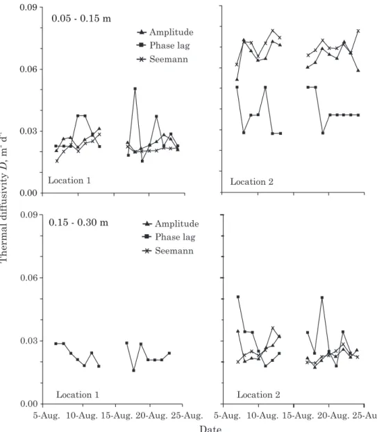
Figure 2. Thermal diffusivity D determined by the amplitude ratio method (Equation 12), the phase lag
the order of 0.03 m2 d-1 at Location 1, i.e., about twice as high as at Location 2. The diffusivities determined by the phase lag method agreed with the values at Location 1, but at Location 2 they were systematically lower (around 0.04 m2 d-1). These values are in agreement with the normally reported magnitude: Bristow et al. (1994) measured thermal diffusivities of around 0.016 and 0.023 m2 d-1 in a clay and a sand soil, respectively; Tessy Chako & Renuka (2002) reported values of around 0.025 and 0.05 m2 d-1 in dry and wet soil, respectively, and Ramana Rao et al. (2005) found values of around 0.04 m2 d-1.
For the layer 0.15-0.30 m, values by the three methods at Location 2 were also similar and in good agreement with each other. At Location 1, however, both the amplitude ratio and the Seemann method resulted in extraordinary high values, i.e., 10 - 20 times higher than those by the phase lag method. The reason is that the temperature differences measured by the sensor in the 0.30 m layer were small and of the same order (around 0.15-0.25 °C) as daily average temperature increase or decrease. Therefore, observations of temperature differences (or minimum and maximum temperatures) during a 24-h period may be highly affected by this daily average variation, resulting in erroneous estimations. In fact, the boundary condition expressed in equation 7 is not met under these conditions. Ramana Rao et al. (2005) found a threefold difference between the amplitude ratio and phase lag method when analysing daily temperature waves.
From this observation, and the fact that the high diffusivities as determined by the amplitude ratio method for Location 2 in the 0.15-0.30 m layer were beyond the normal range for this soil property, it was concluded that the phase lag method is more reliable than the amplitude ratio method under uncontrolled conditions and a temporal temperature gradient, especially in deeper layers where the temperature amplitude is small. We therefore proceeded with the analysis and interpretation of the phase lag method only.
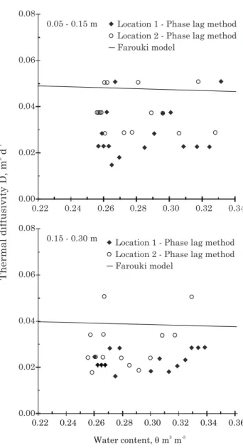
Diffusivity data determined by the phase lag method together with predictions obtained by the soil composition and particle arrangement model of Farouki (1986), as a function of water content, are presented in figure 3. Although the model predictions were in general slightly higher than the measured values, the difference was small and the Farouki (1986) model using values of thermal conductivity for sandstone and kaolinite determined the values of thermal diffusivity in the appropriate order of magnitude. Model predictions were little related with water contentin this range; observations confirmed this, as no trend was observed. In the wetter range of water contents, thermal conductivity increases with water content at about the same rate (or a little slower) than specific heat capacity, therefore diffusivity is to
be expected to remain about constant or decrease slightly with increasing water content (De Vries, 1975; Nobel & Geller, 1987). For the 0.05-0.15 m layer, the average value of D was 0.0335 m2 d-1, with a standard deviation of 0.0107 m2 d-1 (coefficient of variance cv = 32 %); the data analysis of the 0.15-0.30 m layer yielded an average of 0.0266 m2 d-1 and a standard deviation of 0.0085 m2 d-1 (coefficient of variance also being 32 %). These values are all within the range reported elsewhere (Bristow et al., 1994; Tessy Chako & Renuka, 2002; Ramana Rao et al., 2005). The average values for thermal conductivity λ were found to be 77 kJ m-1 d-1 K-1 (0.89 W m-1 K-1) in the upper layer and 59 kJ m-1 d-1 K-1 (0.68 W m-1 K-1) in the subsurface layer.
Figure 3. Thermal diffusivity D determined by the
phase lag method (Equation 14) versus observed
water content θθθθθ for both Locations and both depth intervals. The solid line represents model predictions (Equation 16 divided by Equation 4).
0.00 0.02 0.04 0.06 0.08
0.22 0.24 0.26 0.28 0.30 0.32 0.34
0.00 0.02 0.04 0.06 0.08
0.22 0.24 0.26 0.28 0.30 0.32 0.34 0.36
0.05 - 0.15 m Location 1 - Phase lag method
Location 2 - Phase lag method Farouki model
Location 1 - Phase lag method Location 2 - Phase lag method Farouki model
0.15 - 0.30 m
Thermal diffusivity D, m
d
2
-1
CONCLUSIONS
1. To determine thermal diffusivity for short wave periods (1 day), the phase lag method is more reliable than the amplitude ratio or the Seemann method under uncontrolled conditions, where the temperature gradient is relatively steep over a longer period, especially for deeper layers where temperature variations are small. 2. The proposed method using a daily phase lag between sine waves to obtain the thermal diffusivity resulted in coherent values, similar at both experimental Locations and to values reported in literature.
3. For the soil under investigation, the Farouki (1986) model, based on values of thermal conductivity for sandstone and kaolinite, determined the values of thermal diffusivity in the appropriate order of magnitude.
4. Within the water content range from 0.26-0.34 m3 m-3, the average value of thermal diffusivity was 0.034 m2 d-1 in the top layer (0.05-0.15 m) and 0.027 m2 d-1 in the subsurface layer (0.15-0.30 m).
LITERATURE CITED
ADAMS, W.M.; WATTS, G. & MASON, G. Estimation of thermal diffusivity from field observations of temperature as a function of time and depth. Am. Mineral., 61:560-568, 1976. BAKKER, G.; VAN DER PLOEG, M.J.; DE ROOIJ, G.H.; HOOGENDAM, C.W.; GOOREN, H.P.A.; HUISKES, C.; KOOPAL, L.K. & KRUIDHOF, H. New polymer tensiometers: measuring matric pressures down to the wilting point. Vadose Zone J., 6:196-202, 2007.
BARBER, S.A.; MacKAY, A.D.; KUCHENBUCH, R.O. & BARRACLOUGH, P.B. Effects of soil temperature and water on maize root growth. Plant Soil, 111:267-269, 1988. BOWEN, G.D. Effects of soil temperature on root growth and on phosphate uptake along Pinus radiata roots. Austr. J. Soil Res., 8:31-42, 1970.
BRISTOW, K.L.; KLUITENBERG, G.J. & HORTON, R. Measurement of soil thermal properties with a dual-probe heat-pulse technique. Soil Sci. Soc. Am. J., 58:1288-1294, 1994. CARSLAW, H.S. & JAEGER, J.C. Conduction of heat in solids.
2.ed. Oxford, Oxford University Press, 1959. 510p. CICHOTA, R.; ELIAS, E.A. & DE JONG VAN LIER, Q. Testing
a finite-difference model for soil heat transfer by comparing numerical and analytical solutions. Environ. Modelling Software, 19:495-506, 2004.
DE JONG VAN LIER, Q. & LIBARDI, P.L. Variabilidade dos parâmetros da equação que relaciona a condutividade hidráulica com a umidade do solo no método do perfil instantâneo. R. Bras. Ci. Solo, 23:1005-1014, 1999. DE VRIES, D.A. Heat transfer in soils. In: DE VRIES, D.A. &
AFGAN, N.F., eds. Heat and mass transfer in the biosphere. I. Transfer processes in plant environment. New York, Wiley, 1975. p.5-28.
ELIAS, E.A.; CICHOTA, R.; TORRIANI, H.H. & DE JONG VAN LIER, Q. Analytical soil temperature model: correction for temporal variation of daily amplitude. Soil Sci. Soc. Am. J., 68:784-788, 2004.
FAROUKI, O.T. Thermal properties of soils. California, Trans. Tech., 1986. 136p. (Series on Rock and Soil Mechanics, 11) GAO, Z.; BIAN, L.; HU, Y.; WANG, L. & FAN, J. Determination of soil temperature in an arid region. J. Arid Environ., 71:157-168, 2007.
GEMANT, A. The thermal conductivity of soils. J. Appl. Phys., 21:750-752, 1950.
HORTON, R.; WIERENGA, P.J. & NIELSEN, D.R. Evaluation of methods for determining the apparent thermal diffusivity of soil near the surface. Soil Sci. Soc. Am. J., 47:25-32, 1983.
KIRKHAM, D. & POWERS, W.L. Advanced soil physics. 2.ed. New York, Wiley Interscience, 1972. 534p.
KIZITO, F.; CAMPBELL, C.S.; CAMPBELL, G.S.; COBOS, D.R.; TEARE, B.L.; CARTER, B. & HOPMANS, J.W. Frequency, electrical conductivity and temperature analysis of a low-cost capacitance soil moisture sensor. J. Hydrol., 352:367-378, 2008.
MICHOT, A.; SMITH, D.S.; DEGOT, S. & GAULT, C. Thermal conductivity and specific heat of kaolinite: Evolution with thermal treatment. J. Eur. Ceramic Soc., 28:2639-2644, 2008. NAGEL, K.A.; KASTENHOLZ, B.; JAHNKE, S.; VAN DUSSCHOTEN, D.; AACH, T.; MÜHLICH, M.; TRUHN, D.; SCHARR, H.; TERJUNG, S.; WALTER, A. & SCHURR, U. Temperature responses of roots: impact on growth, root system architecture and implications for phenotyping. Func. Plant Biol., 36:947-959, 2009.
NOBEL, P.S. & GELLER, G.N. Temperature modelling of wet and dry desert soils. J. Ecol., 75:247-258, 1987.
PASSERAT DE SILANS, A.; DA SILVA, F.M. & BARBOSA, F.A.R. Determinação in loco da difusividade térmica num solo da região de caatinga (PB). R. Bras. Ci. Solo, 30:41-48, 2006.
PREVEDELLO, C.L. Determinação da difusividade térmica de meios porosos. R. Bras. Ci. Solo, 17:319-324, 1993. RAMANA RAO, T.V.; DA SILVA, B.B. & MOREIRA, A.A.
Características térmicas do solo em Salvador, BA. R. Bras. Eng. Agríc. Amb., 9:554-559, 2005.
ROSENBAUM, U.; HUISMAN, J.A.; WEUTHEN, A.; VEREECKEN, H. & BOGENA, H.R. Sensor-to-sensor variability of the ECH2O EC-5, TE, and 5TE sensors in dielectric liquids. Vadose Zone J., 9:181-186, 2010. SEEMANN, J. Measuring technology. In: SEEMANN, J.;
CHIRKOV, Y.I.; LOMAS, J. & PRIMAULT, B., eds. Agrometeorology. Berlin, Springer-Verlag, 1979. p.40-45. TESSY CHACKO, P. & RENUKA, G. Temperature mapping, thermal diffusivity and subsoil heat flux at Kariavattom of Kerala. Proc. Indian Acad. Sci. (Earth Planet. Sci.), 111:79-85, 2002.