Determining the In Situ Apparent Thermal Diffusivity of a Sandy Soil

* Corresponding author: E-mail: ossilva@uv.mx

Received: February 10, 2018 Approved: June 29, 2018

How to cite: Silva-Aguilar OF, Andaverde-Arredondo JA, Escobedo-Trujillo BA, Benitez-Fundora AJ. Determining the in situ apparent thermal diffusivity of a sandy soil. Rev Bras Cienc Solo. 2018;42:e0180025.

https://doi.org/10.1590/18069657rbcs20180025

Copyright: This is an open-access article distributed under the terms of the Creative Commons Attribution License, which permits unrestricted use, distribution, and reproduction in any medium, provided that the original author and source are credited.

Determining the

In Situ

_Apparent

Thermal Diffusivity of a Sandy Soil

, Jorge Alberto Andaverde Arredondo(2)

, Beatris

Adriana Escobedo Trujillo(2) and Artemio Jesús Benitez Fundora(2)

(1)

National Autonomous University of Mexico, Department of Postgraduate in Engineering, Renewable Energy Institute, Temixco, Morelos, Mexico.

(2)

University of Veracruz, Coatzacoalcos, Veracruz, Mexico.

ABSTRACT: The thermal wave amplitude method is used to determine soil thermal

diffusivity in situ for a sandy soil in Mexico (Coatzacoalcos, Veracruz). Soil diurnal temperature fluctuations were measured from depths of 0.05 to 0.65 m, in 0.01 m increments, during the months of April and August. Five mean diffusivity values were obtained experimentally, corresponding to the different depths combination. The soil thermal diffusivity ranged between 2.26 × 10-7

and 8.71 × 10-7

m2

s-1

. The diffusivity values obtained are within the absolute ranges reported in the literature. A positive linear effect between the diffusivity values and depth was observed on a homogeneous sandy soil. These increments are due to the soil moisture variations and the volumetric calorific capacity of the soil. An uncertainty analysis was made to validate our results, resulting in a relative standard deviation with values in the range of 4.51 to 27.37 %. The uncertainties of 0.49 to 26.66 % RSD in the amplitude of the thermal wave are the factor that contributes most to the propagation of errors of the diffusivity.

Keywords: geothermal, thermal properties, conductivity, error propagation.

INTRODUCTION

Soil thermal properties are important for a variety of purposes such as hydrological, agricultural, and geological studies, as well as applications in geothermal heat exchangers. The thermal conductivity K (J s-1 m-1 K-1) and the volumetric heat capacity CV (J m

-3

K-1) often constitute the input data for heat flow and soil water models (Ochsner et al., 2001; Sanner et al., 2005). These properties, when combined, result in thermal diffusivity α (m2

s-1), depending on the mineral components, porosity, and the soil water content. Note that the values of the soil thermal properties reported in the literature are not consistent. Therefore, it is advisable to obtain site-specific values when possible (Spitler et al., 2000). The thermal conductivity has the most effect on soil heat transfer when compared to the other soil thermal properties (Florides and Kalogirou, 2004; Demir et al., 2009). Moreover, Pouloupatis et al. (2011) emphasize an important soil property known as the geothermal gradient, which measures the rapid temperature increments by the constant flow of heat produced by the thermal conductivity of the soil.

Thermal conductivity and diffusivity values are obtained from measurements of the temperature variation in materials (Beardsmore and Cull, 2001). To achieve that, several techniques have been developed that can be classified as in the laboratory or in situ. Both methods are based on the concept of thermal waves, which was proposed by Angstrom in 1861. It involved subjecting a sample to periodic temperature variations, where one end is heated and the opposite end is cooled. Meanwhile, temperature measurements are made locally at different distances along the axis of the sample. Angstrom’s original idea was adapted by many researchers to determine the thermal diffusivity (Bodzenta, 2008).

In situ techniques have been developed with the aim of carrying out field measurements in order to preserve the natural soil conditions without requiring sample preparation. The

thermal stimulus for in situ techniques can be natural or artificial. The natural thermal

stimulus measures the variation of surface temperature. The insertion of thermal devices or fluids of a known temperature into varying depths in the ground and the observation of temperature variation over time measures the artificial variation of temperature.

Some of the best known in situ methods used in order to calculate the apparent thermal

diffusivity at low depth are:

(a) Analytical and numerical methods (finite differences). The analytical methods: amplitude, phase, arctangent, and logarithmic in an explicit way require little information. The authors reported that diffusivity was calculated up to 0.10 m depth of the soil (Horton et al., 1983).

(b) Amplitude method. Uses the periodic variation of the surface thermal wave, resulting from daily weather variation, a natural heat source (Horton et al., 1983). The amplitude method has the best results when determining the apparent thermal diffusivity of the soil, after comparing the amplitude, phase, tangent, logarithmic, and harmonic equation methods. Thermal diffusivity values were calculated for the upper 0.10 m of soil, assuming that the soil was uniform. The results showed an increase of diffusivity by increasing the soil moisture (Verhoef et al., 1996). The amplitude method was used by Evett et al. (2012) to determine the apparent thermal diffusivity of soil with artificial heat sources using plates at depths of 0.02 to 0.16 m. In later studies by Danelichen et al. (2013), this method was used as a pattern to compare the results of the amplitude, phase, arctangent, and logarithmic methods in order to determine the apparent thermal diffusivity of the soil. In this study the diffusivity was calculated up to 0.15 m depth.

soils. Thermal soil values were obtained for non-uniform soils up to a depth of 0.20 m (Nassar and Horton, 1990).

The amplitude method is taken as a standard. Hence, the current research aimed to determine the values of apparent diffusivity of sandy soil up to depths of 0.55 m using this method. The degree of uncertainty in the estimated values was analyzed to evaluate whether it is suitable to continue using it as a reference. So, the thermal diffusivity obtained will be used to design for horizontal geothermal exchanges in sandy soil areas near the beach, which are installed at depths of up to 2 m (Florides and Kalogirou, 2007). This design is intended for energy saving purposes related to cooling for human comfort. In order to design horizontal geothermal exchangers that operate under a more or less fixed water content distribution, it can be used to determine the thermal diffusivity without considering the moisture soil content. In fact, Demir et al. (2009) used the soil thermal diffusivity and temperature in their design calculations without specifying the moisture content.

MATERIALS AND METHODS

The experiment was conducted in Coatzacoalcos, Veracruz, Mexico, within the facilities of the Universidad Veracruzana, which is located at latitude 18° 08’ 39” N, longitude 94° 28’ 36” W and 10 m above sea level. The university is located in a coastal zone of the Gulf of Mexico, where the warm, humid tropical climate prevails, with an average annual maximum temperature of 29.2 °C, average annual minimum temperature of 22.9 °C, average temperature of 26.1 °C, and a relative humidity annual average of 78 % (National Meteorological System, 2013). The properties of the soil stratigraphy at experimental depths are 93 % of sand and 7 % of silt. The composition of the soil varied only slightly in the seven levels of measurement, so it was considered as homogeneous. It contained graded silty sand, with a gradual increase in the degree of compaction. The soil exhibits no plasticity and lacks fine materials. The groundwater levels were generally between 1 and 2 m from the surface.

Equipment

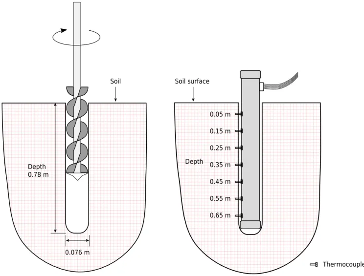
A 0.7 m watertight measuring probe with temperature sensors at intervals of 0.1 m was built with polyvinyl chloride (PVC) pipe and connectors. The temperature sensors consisted of Copper-Constantan T type thermocouples, with an AMETEK CTC-140 model. The standard thermocouple was verified with a calibration error of about ± 0.02 °C and the remainder were adjusted in a water bath. Sensor data logging with data acquisition by Agilent 34972A was completed.

The sensor installation site selected was a shaded patch, away from foundations, pipelines, and drains. We aimed to keep disturbance to a minimum during the drilling process, hoping for no soil compaction. To achieve that, a 0.076 m-diameter twist drill was used to provide a perfect fit for the probe, including the temperature sensors. It was assumed that the temperature sensors made direct contact with the soil material, as shown in figure 1.

Experiments

Temperature measurements were conducted in April and August 2013. Those dates were selected to obtain measurements in the month of highest average annual temperature (April) and in the month of declining temperatures (August) prior to the two-month period where a higher rainfall in the area was expected. The depth of application was from 0.05 to 0.65 m. Experiments lasted up to 96 h with a temperature measurement frequency of 15 seconds.

Mathematical model and uncertainty analysis

We now show a solution to the heat equation subject to certain boundary conditions with the aim of analyzing the variation in temperature at different depths of soil, which will allow us to obtain a formula for the thermal diffusivity. The main sources are Carslaw and Jaeger (1959), Beardsmore and Cull (2001), and Bevington and Robinson (2003).

Unidirectional heat flow evolves according to Fourier’s differential equation (Equation 1):

1 α = ∂2

T ∂z2

∂T

∂t Eq. 1

in which T is the temperature (K), z is the depth (m), α is the thermal diffusivity (m2

s-1), and t is time (s).

The solution to equation 1 by Carslaw and Jaeger (1959) for penetrating into the ground of a periodic oscillation of the temperature (not necessarily at the soil surface) at depth

z, is given through the equation 2:

Thermocouple Soil surface

Soil

Depth

0.076 m Depth

0.78 m

0.65 m 0.55 m 0.45 m 0.35 m 0.25 m 0.15 m 0.05 m

T(t,z) = Tz +

Σ

n=1Ane

–z√nω/2α _{sin(nωt – φ}

n – z

√

In which Tz is the average temperature at depth z; ω is the frequency; and φn is the partial phase wave. The attenuation of the wave amplitude with respect to depth is given by An. If the frequency ω is replaced by an equivalent period (2π/T) and depth z is taken at two discrete levels Z1 and Z2, equation 2 becomes equation 3:

Z2 – Z1

1n AZ1 – 1n AZ2

α = π T

2

Eq. 3

To validate the estimated thermal diffusivity values, we proposed:

(a) To verify the theoretical formula for the variation of temperature at several depths T(t, z), see equation 2. If our estimated diffusivities are valid, then equation 3 and the experimental temperatures must coincide. To this end, we plot the experimental temperature data at a depth z = 0.05 m. Next, we make a trigonometric interpolation of sine functions (i.e., sine Fourier series) (Equation 4):

F(t) = Tz +

Σ

i=0Ai sin(wit + ψ) Eq. 4

with the objective of finding the Fourier series that best fits this experimental temperature data and thus to estimate the values of Ai, wi, and ψ.

(b) Uncertainty analysis. The estimation of the thermal diffusivity with equation 3 could be affected by errors due to the instrumentation or methodology used. Hence, an uncertainty analysis was conducted to assess the confidence in the results using equation 5:

[

]

α = π

T

Eq. 5

In which X1 = AZ1/AZ2, X2 = 1n X1, X3 = (Z2 – Z1), and X4 = X3/X2.

This equation allows us to find the general equation of error propagation for the thermal diffusivity S_α (Equation 6), since it is possible to apply the error propagation

formulas proposed by Bevington and Robinson (2003) to the variables X1, X2, X3, and

X4. In fact,

S2

Z2 + S 2

Z1

(Z2 – Z1) 2

S_α ≈ 2 α

S2

AZ2

A2Z2

S2

AZ1

AZ21

+

+

AZ1

AZ2

1n

2

Eq. 6

where SZ is the depth error, and SAz is the wave amplitude error.

RESULTS

The experiments carried out in April and August 2013 contributed the graphical results that record the temperature variation of both experiments for each of the depths and are shown in figures 2 and 3.

Soil temperature

The temperature is shown in figures 4a and 4b for a 24-hour period in April and August, respectively. Each line represents a particular time of the day. It is shown that for the near-surface sensor (0.05 m) the temperature is in the range of 29-45 °C in April and of 30-38 °C in August. At greater depths, the temperature range reduces and they are imperceptible at 0.55 m. It is apparent that at greater depths of measurement the temperatures have a substantial reduction in amplitude and are almost constant near 28 °C.

In the experimental results from the amplitude of the thermal wave in a period of 24 h (Figure 5), the amplitude error for all periods is considered constant, because it is directly dependent on the thermocouple error. It is also considered that exists uncertainty at a depth of ± 0.5 mm, that is to say, SZ ± 0.5 mm, because it is the one that corresponds

to the tool used in the measurement.

Figures 5a and 5b show the amplitudes of the thermal waves with depth, during the months of April and August, respectively. The trend lines obtained between amplitude and depth adjust to a line type trend. Error bars are not shown due to their limited size.

Temperature (°C) Time (h) 0.05 m 25 0.15 m 0.25 m 0.35 m 0.45 m 0.55 m 0.65 m 30 35 40 45 50 96 90 84 78 72 66 60 54 48 42 36 30 24 18 12 6

Figure 2. Temperature variation in soil at different depths with time, experiment from April 15-19,

2013 at the Universidad Veracruzana Campus Coatzacoalcos, Veracruz, Mexico.

Temperature (°C) Time (h) 0.05 m 28 0.15 m 0.25 m 0.35 m 0.45 m 0.55 m 0.65 m 30 32 36 38 40 90 84 78 72 66 60 54 48 42 36 30 24 18 12 6 34

Figure 3. Temperature variation in soil at different depths regarding time. This experiment was conducted

The apparent thermal diffusivity values obtained by using temperatures at different depths (Equation 3) together with their uncertainty are shown in table 1.

Diffusivity increases in proportion to the increase of the distance between thermocouples, and the relative similarity of results between periods of the same experiment. The increase 0.7

Temperature (°C) (a)

Depth (m)

0.6 0.5 0.4 0.3 0.2 0.1 0.0

26 28 30 32 34 36 38 40 42 44 46

Temperature (°C) (a)

26 28 30 32 34 36 38 40 42 44 46

Figure 4. The geothermal profile of the soil where each line corresponds to a certain time of day. The maximum recorded depth is

0.65 m and the recorded dates are (a) April 16, 2013 and (b) August 9, 2013.

Figure 5. Variation of the thermal wave amplitude with respect to soil depth. The trend line is a potential equation. The error bars are

not significant because of its size. a) Letters A, B, and C correspond to April 15, 16, and 17, 2013. b) Letters D, E, and F correspond

to August 7, 8, and 9, 2013.

Amplitude (°C)

Depth (m) 0.05

0

0.15 0.25 0.35 0.45 0.55

2 4 6 8 10 12

A

B

C (a)

Amplitude (°C)

Depth (m) 0.05

0

0.15 0.25 0.35 0.45 0.55

1 2 3 4 5 6

D

E

in error as the diffusivity is increased can be explained via equation 4, since the error is proportional to the diffusivity as well as the fact that for lower temperatures it is more difficult to determine peaks.

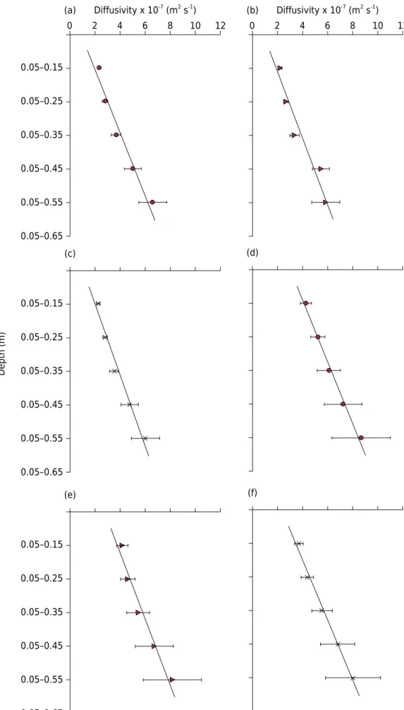
The results of the diffusivities and uncertainties are shown in figure 6. The apparent diffusivity of the soil increases linearly as shown by the trend line. This is due to the fact that by combining the shallow sensor with ever deeper sensors, it is taking more and more of the deeper soil into account where the moisture content of the soil will be higher.

Linear regressions between the depth and the apparent diffusivity were made. Intercept values a, slope b, and an r linear correlation are shown in table 2. It can be seen that the trend lines are similar in slope between 0.943 and 1.117 and the r correlation coefficient is between 0.928 and 0.990. This shows a strong correlation among the variables analyzed, at least for the experimental range.

The increasing thermal diffusivity with depth is related to the increased moisture at greater depths. As mentioned before, the ground water level of the sand pack is located 1.5 m beneath the surface of the soil. In this paper, the relationship between diffusivity and moisture is not reported. It only focuses on the application of the method and the propagation of errors.

In equation, TZ is considered the mean experimental temperature with z = 0.05 m. The

graph of the Fourier series of n = 8595 vs the experimental temperature at a depth z = 0.05 m is presented at figure 7a. Observe that with 8595 harmonics, a good fit is obtained with a correlation coefficient of r =0.999 (Figure 8a).

Now, replacing the values of Ai, wi, and ψ obtained by means of the interpolation in the Fourier series (with z = 0.05 m) and the experimental diffusivity values (Table 2) in equation 4, this shows the theoretical formula for the variation of temperature at different depths. Figures 7b and 7c show the comparison of the theoretical and experimental temperature at depths z = 0.15 and 0.25 m, respectively. It can be observed that the theoretical and the experimental temperature show a good fit, since the correlation coefficients are

r = 0.92 and 0.85 for the depths z = 0.15 and 0.25 m, respectively (Figures 8b and 8c).

Table 1. Apparent diffusivity calculated α × 10-7

(m2 s-1) with their respective error ranges at different soil depths in April 2013 (A, B, and C) and August 2013 (D, E, and F)

ΔZ A B C D E F

Apparent diffusivity(1)

α × 10-7

m m2 _s-1

0.05-0.15 2.37 ± 0.11 2.26 ± 0.11 2.30 ± 0.10 4.31 ± 0.44 4.12 ± 0.39 3.74 ± 0.35 0.05-0.25 2.82 ± 0.19 2.73 ± 0.19 2.80 ± 0.18 5.26 ± 0.58 4.55 ± 0.50 4.41 ± 0.48 0.05-0.35 3.71 ± 0.37 3.38 ± 0.38 3.54 ± 0.36 6.15 ± 0.92 5.40 ± 0.84 5.60 ± 0.83 0.05-0.45 5.04 ± 0.68 5.50 ± 0.72 4.77 ± 0.66 7.29 ± 1.50 6.69 ± 1.40 6.86 ± 1.38 0.05-0.55 6.58 ± 1.11 5.87 ± 1.22 6.03 ± 1.11 8.71 ± 2.34 8.15 ± 2.23 8.10 ± 2.19 (1) _{The thermal wave amplitude method was used to determine the apparent diffusivity.}

Table 2. Diffusivity-depth linear regression parameters

A B C D E F

Linear regression parameters

a 0.912 0.951 1.059 3.095 2.722 2.391

b 1.064 0.999 0.943 1.083 1.020 1.117

Depth (m)

Diffusivity x 10-7 _(m2 _s-1₎ (a)

0 2 4 6 8 10 12

0.05–0.65 0.05–0.55 0.05–0.45 0.05–0.35 0.05–0.25 0.05–0.15

(c)

0.05–0.65 0.05–0.55 0.05–0.45 0.05–0.35 0.05–0.25 0.05–0.15

(e)

0.05–0.65 0.05–0.55 0.05–0.45 0.05–0.35 0.05–0.25 0.05–0.15

Diffusivity x 10-7 _(m2 _s-1₎ (b)

0 2 4 6 8 10 12

(d)

(f)

Figure 6. Columns of the apparent soil diffusivity calculated at different depths, with error bars

DISCUSSION

The amplitudes of the waves decrease in the depth close to an exponential (Figure 5). However, it is possible to determine and therefore use this method of amplitude for this type of soil to a depth of 0.55 m, it has been previously used on varying soil types and depths by Horton et al. (1983), Verhoef et al. (1996), Evett et al. (2012), and Danelichen et al. (2013).

The diffusivity values increase when there is a higher soil thickness (Figure 6). This can be explained because the moisture is higher at increased depth and therefore the thermal diffusivity increases. This increment in humidity–diffusivity coincides with findings from Verhoef et al. (1996) and Florides and Kalogirou (2004). The values reported by Florides and Kalogirou (2004) are 1 × 10-7

to 10 × 10-7

m2

s-1

. In the present work, the apparent thermal diffusivity values of the sandy soil were between 2.26 × 10-7

and 8.71 × 10-7

m2

s-1

, in the aforementioned interval.

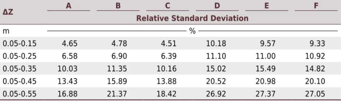
On the other hand, the change of the values of thermal diffusivity of the soil with depth was mentioned as having a linear correlation, with coefficients close to one. Table 3. Percentage of error calculated the apparent diffusivity experiments April and August 2013

ΔZ A B C D E F

Relative Standard Deviation

m %

0.05-0.15 4.65 4.78 4.51 10.18 9.57 9.33

0.05-0.25 6.58 6.90 6.39 11.10 11.00 10.92

0.05-0.35 10.03 11.35 10.16 15.02 15.49 14.82

0.05-0.45 13.43 15.89 13.88 20.52 20.98 20.10 0.05-0.55 16.88 21.37 18.42 26.92 27.37 27.05

Figure 7. Comparison of theoretical and experimental variation of temperature (a) z = 0.05 m, (b) z = 0.15 m, (c) z = 0.25 m.

Simulation Experimental

Time (day) 0.0

Simulation Experimental Simulation

Experimental

(a) (b) (c)

0.5 1.0 1.5 2.0 2.5 3.0

0.0 0.5 1.0 1.5 2.0 2.5 3.0 0.0 0.5 1.0 1.5 2.0 2.5 3.0

28 30 32 34 36 38 40 42 44 46

Temperature (°C)

30 32 33 34 35 36

31

30 31 31.5 32 32.5 33

This might be related to increased humidity with increasing depth. This situation is expected, as there are records of nearby wells where the groundwater is at depths of 1 to 2 m.

In terms of the uncertainty values calculated from the propagation of errors observed in table 4, the relative standard deviation values increased with depth by values of 4.65 up to 27.37 %. These uncertainty values are high, and they could be lower if the uncertainties of the wave amplitudes decrease, since this is the parameter that has the greatest impact on the value of the propagation of errors, the values of % RSD being between 0.49 and 26.66 %.

Because it is more difficult to measure the amplitude of the wave in soil of greater depth, we consider that 0.55 m is the limit of the depth of this type of soil when using this method, with diurnal fluctuations of temperature.

CONCLUSIONS

The apparent soil diffusivity values for a Mexican sandy soil obtained by the attenuation method of the thermal wave amplitude varied from 2.26 × 10-7

to 8.71 × 10-7

m2 s-1, which are within the range of values reported in the literature for sand at varying soil moisture content.

The experimental design and method used allowed us simultaneously to obtain multiple values of apparent diffusivity at different depths in one measurement cycle, and gave us the uncertainties of the diffusivity values obtained.

A linear trend of the apparent diffusivity was obtained in the experimental soil depth interval, as the depth increases, with a linear correlation in the range of 0.928-0.990. The increase in the values of thermal diffusivity in proportion to the depth is related to the gradient of moisture. However, it will be convenient in future work to measure the

Figure 8. Linear regression model, theoretical temperature = a + b (experimental temperature).

Simulation (°C)

Experimental (°C) 25

28

30 35 40 45

30 32 34 36 38 40 42 44 46

30 31 32 33 34 35 36

30 30.5 31 31.5 32 32.5 33

30 31 32 33 34 35 36 30 30.5 31 31.5 32 32.5 33

moisture at the same points of temperature measurement so as to establish convincingly the value of the thermal diffusivity of soil moisture.

The method has the limitation of only being able to evaluate the apparent diffusivity at depths less than one meter. This limitation is due to the use of natural thermal wave disturbance, which tends to stabilize in relation to depth.

Uncertainty of the wave amplitude is the parameter that contributes most to the uncertainty of the soil thermal diffusivity, but can decrease if the measurements are made with more precise equipment.

It is suggested not only that the design of geothermal exchangers that do not require moisture content should be taken into account in subsequent research, but also that the simultaneous measurement of temperature and soil moisture is carried out to establish a theoretical model that fits the experimental results with the two variables.

ACKNOWLEDGMENTS

We would like to thank the reviewers and the editors for all the useful comments on this paper, and especially Dr. Anne Verhoef for her outstanding job on her feedback that helped us to improve this manuscript, and F. Alejandro Alaffita Hernández for his help with graphic design. Also, we wish to give a special mention to the Energy Laboratory and the Center of Research in Energy and Sustainable Resources of the University of Veracruz for allowing us to use their equipment and facilities for the completion of this experiment.

REFERENCES

Beardsmore GR, Cull JP. Crustal heat flow: a guide to measurement and modelling. Cambridge:

Cambridge University Press; 2001.

Bevington PR, Robinson DK. Data reduction and error analysis: for the physical sciences. 3rd ed. Boston: Mc-Graw Hill; 2003.

Bodzenta J. Thermal wave methods in investigation of thermal properties of solids. Eur Phys J Special Topics. 2008;154:305-11. https://doi.org/10.1140/epjst/e2008-00566-5

Carslaw HS, Jaeger JC. Conduction of heat in solids. 2nd ed. Oxford: Oxford University Press; 1959.

Danelichen VMH, Biudes MS, Souza MC, Machado NG, Curado LFA, Nogueira JS. Soil thermal

diffusivity of Gleyc Solonetz soil estimated by different methods in the Brazilian Pantanal. Open

Journal of Soil Science. 2013;3:15-22. https://doi.org/10.4236/ojss.2013.31003

Demir H, Koyun A, Temir G. Heat transfer of horizontal parallel pipe ground heat

exchanger and experimental verification. Appl Therm Eng. 2009;29:224-33.

https://doi.org/10.1016/j.applthermaleng.2008.02.027

Evett SR, Agam N, Kustas WP, Colaizzi PD, Schwartz RC. Soil profile method for soil thermal diffusivity, conductivity and heat flux: comparison to soil heat flux plates. Adv Water Resour.

2012;50:41-54. https://doi.org/10.1016/j.advwatres.2012.04.012

Florides G, Kalogirou S. Ground heat exchangers - a review of systems, models and applications. Renew Energ. 2007;32:2461-78. https://doi.org/10.1016/j.renene.2006.12.014

Florides G, Kalogirou S. Measurements of ground temperature at various depths. In: Proceedings of the 3rd International Conference on Sustainable Energy Technologies; Nottingham, UK; 2004.

Horton R, Wierenga PJ, Nielsen DR. Evaluation of methods for determining the

apparent thermal diffusivity of soil near the surface. Soil Sci Soc Am J. 1983;47:25-32.

https://doi.org/10.2136/sssaj1983.03615995004700010005x

Nassar IN, Horton R. Determination of soil apparent thermal diffusivity from

National Meteorological System, National Water Commission [accessed on 2013 Apr 10]. Available at: http://smn.cna.gob.mx/observatorios/historica/coatzacoalcos.pdf

Ochsner TE, Horton R, Ren T. A new perspective on soil thermal properties. Soil Sci Soc Am J. 2001;65:1641-7. https://doi.org/10.12691/aees-2-2-4

Pouloupatis PD, Florides G, Tassou S. Measurements of ground temperatures in Cyprus for ground thermal applications. Renew Energ. 2011;36:804-14. https://doi.org/10.1016/j.renene.2010.07.029

Sanner B, Hellström G, Spitler J, Gehlin S. Thermal response test - current status and world-wide application. In: Proceedings World Geothermal Congress; Antalya, Turkey; 2005.

Spitler JD, Yavuzturk C, Rees SJ. In situ measurement of ground thermal properties. In: Proceedings of the Terrastock; Stuttgart; 2000. p. 165-70.