Telmo Ivani Costa Carvalho Barros

Licenciado em Ciências de Engenharia Eletrotécnica e de Computadores

Data Acquisition Channel for an E-Nose

Dissertação para obtenção do Grau de Mestre em

Engenharia Electrotécnica e de Computadores

for an Electronic Nose

Copyright © Telmo Ivani Costa Carvalho Barros, Faculty of Sciences and Technology, NOVA University Lisbon.

The Faculty of Sciences and Technology and the NOVA University Lisbon have the right, perpetual and without geographical boundaries, to file and publish this dissertation through printed copies reproduced on paper or on digital form, or by any other means known or that may be invented, and to disseminate through scientific repositories and admit its copying and distribution for non-commercial, educational or research purposes, as long as credit is given to the author and editor.

Este documento foi gerado utilizando o processador (pdf)LA_{TEX, com base no template “novathesis” [1] desenvolvido no Dep. Informática da FCT-NOVA [2].}

This dissertation represents more than just a piece of paper for me. It is the culmination of six amazing years where I grew not only as a student, but also as a person. This project would not be possible without the guidance of my mentor, Professor Nuno Paulino as well as the help of my colleagues at the Chemical Department, Gonçalo Santos and Ana Carolina Pádua, from the Faculty of Sciences and Technology of the Nova University of Lisbon. They have always demonstrated openness to any question I could’ve had and supported me to pursue this ordeal even when I felt a little disorientated.

Once again, I would like to thank my advisor. Professor Nuno Paulino had an im-mensely great amount of patience and always showed availability to help me.

To Professor Helena Fino, I would also like to thank because she showed me, uninten-tionally, that it is possible to grow up career wise and still maintain her own simplicity and humbleness.

I would also like to thank Professor Rui Tavares for his constant good sense of humour, something that tends to be forgotten once the workload increases.

To my great group of friends, I want to say thank you so much. You are definitely one of the main reasons I’m achieving so much.

I would also love to thank my mother and sister for being my foundation. Everything good I do is with them on my mind first.

Nowadays, electronic devices are ubiquitous. This spread across all scientific fields has allowed for greater development of solutions for problems once thought impossible, or impractical, to solve. Most specifically, it leads to a constant cost reduction in previously expensive technology, to a point where university students can acquire these devices and tinker with them, even finding applications that were not initially thought for the device. As a result, we began the development of this e-nose system, since it became increasingly important to know and understand the constituents and source of a chemical sample.

This dissertation arises from the need to integrate the computational power inherent to a low-cost microcontroller unit, to identify chemical substances and their character-istics. With the main goal set, it was possible to formulate the guidelines to achieve a successful data acquisition channel for an e-nose system implementation with reduced costs, size and fast execution. The starting point consisted in understanding how previ-ous implementations of this system work, as well as its most basic components. After researching and studying e-nose technologies, I was able to define two separate segments for a data acquisition channel: acquisition & communication module (hardware) and a data pre-processing module (software). By using a conductive polymer sensor with a PSoC 5LP microcontroller unit, it was possible to detect changes in the sensor response according to the chemical sample being tested, acquire this signal with the Delta Sigma ADC and, straight away, send this data to the computer where it would be pre-processed.

This stage was implemented in Python and with its extensive signal processing li-braries. Its main goal was to receive and store the data so that it could be use on a future pattern recognition algorithm to reach the final e-nose conclusion. Since this displayed to the user, a GUI was developed, and the resulting acquisitions could be displayed in several plots, as a way of verifying a successful operation.

In the end, it was a success, since after performing acquisition, communication and displaying the results, subtle diff_{erences were visible on the plots displayed.}

Atualmente, os dispositivos eletrónicos são omnipresentes. Esta disseminação nos diversos campos científicos permitiu um maior desenvolvimento de soluções para proble-mas que antes eram considerados impossíveis ou impraticáveis de resolver. Mais especi-ficamente, leva a uma constante redução do custo da tecnologia, ao ponto de estudantes universitários poderem adquirir estes dispositivos e trabalhar com eles, até mesmo encon-trar soluções que não foram inicialmente pensadas para o dispositivo. Como resultado, iniciamos o desenvolvimento deste sistema nariz eletrónico, uma vez que se tornou cada vez mais importante conhecer e compreender os constituintes e a fonte de uma amostra química.

Esta dissertação surge da necessidade de integrar o poder computacional inerente a um microcontrolador de baixo custo, para identificar substâncias químicas e as suas características. Com o objetivo principal traçado, foi possível formular as diretrizes para obter um canal de aquisição de dados bem-sucedido para a implementação de um sistema de nariz eletrónico com custos e tamanho reduzidos e execução rápida. O ponto de partida consistiu em compreender implementações anteriores deste sistema, bem como quais os componentes fundamentais. Depois de pesquisar e estudar as tecnologias do nariz eletrónico, consegui definir dois segmentos para um canal de aquisição de dados: módulo de aquisição e comunicação (hardware) e um módulo de pré-processamento de dados (software). Utilizando um sensor deconductive polymercom um microcontrolador PSOC 5LP, foi possível detetar alterações na resposta do sensor de acordo com a amostra química, adquirir este sinal com o ADC Delta Sigma e, seguidamente, enviar estes dados para o computador onde seriam pré-processados.

Esta fase foi implementada em Python e com as suas extensas bibliotecas de proces-samento de sinais. O principal objetivo consistiu em receber e armazenar os dados para que pudessem ser utilizados num futuro algoritmo de reconhecimento de padrões para chegar à conclusão final do nariz eletrónico. Sendo este módulo exibido ao utilizador, foi desenvolvida uma GUI e as aquisições resultantes são exibidas em vários gráficos, como forma de verificar que o processo foi efetuado com sucesso.

List of Figures xiii

List of Tables xv

Acronyms xvii

1 Introduction 1

1.1 Motivation . . . 1

1.1.1 Goals . . . 2

1.2 Thesis Outline . . . 5

2 State-of-the-Art 7 2.1 Electronic Nose . . . 7

2.2 Electronic nose structure . . . 10

2.2.1 Sensors . . . 10

2.2.2 Data Acquisition Channel . . . 16

2.3 System-on-Chip . . . 19

2.3.1 Identification Software . . . 27

2.4 Electronic nose past implementations. . . 27

2.4.1 Identification of cannabis-based drugs . . . 28

2.4.2 Identification of spoiled beef. . . 29

2.4.3 Healthcare application . . . 31

3 Implementation 35 3.1 Data Acquisition and Transmission . . . 36

3.2 Data Pre-processing . . . 47

3.3 Transfer Function . . . 53

3.4 Data acquisition channel flowchart . . . 53

4 Results 57 4.1 Plot results . . . 58

5.2 Future Developments . . . 65

Bibliography 67

A Microcontroller Configuration Code 71

B USB configuration code 77

C Start Screen of the Application code 81

D Start Screen of the Application code 87

E Data Acquisition Implementation code 93

1.1 e-nose . . . 2

1.2 rc circuit . . . 2

1.3 rc circuit charging step response. . . 3

1.4 rc circuit discharging step response . . . 3

2.1 Cross-section of the skull, showing the location of the olfactory epithelium, sensory neurons, cribriform plate, olfactory bulb, and some central connec-tions [14] . . . 8

2.2 Comparison between a mammalian and E-nose systems . . . 9

2.3 Principle of sensors used in E-nose sensing [8] . . . 11

2.4 Photograph of the metal electrodes coated with the conductive polymer . . . 13

2.5 Conductive polymer structure . . . 14

2.6 Conductive Polymer Conductivity . . . 14

2.7 Sample-and-hold circuit . . . 16

2.8 Sample-and-hold time diagram . . . 17

2.9 SAR ADC . . . 17

2.10 ∆Σ_{ADC diagram . . . . 18}

2.11 Arduino UNO . . . 21

2.12 Block diagram of the ATmega328 . . . 21

2.13 MSP430 board . . . 22

2.14 MSP430 block diagram . . . 22

2.15 FRDM-KE06Z . . . 23

2.16 FRDM-KE06Z block diagram . . . 23

2.17 PSoC 5LP . . . 24

2.18 PSoC 5LP architecture . . . 25

2.19 Electrical conductance of TGS842sensor towards exposures to studied drugs[6] 29 2.20 A typical raw signal|response of an electronic nose’s sensor[13] . . . 30

2.21 Overview of Optical e-nose (the side view of the chamber only shows 2 sensors out of 4)[4] . . . 32

2.22 Sensor response to CH4 gas with diff_{erent concentrations starts from 2.5 ppm} to 100 ppm in two wavelengths 7.88µm (left) & 3.4µm (right).[4] . . . 32

3.2 Conductive Polymer Structure . . . 36

3.3 Conductive Polymer sensor response to rectangular wave . . . 38

3.4 RC filter schematic and breadboard implementation . . . 39

3.5 DelSig ADC component . . . 40

3.6 DelSig ADC component configuration . . . 41

3.7 DAC component . . . 42

3.8 DAC component configuration . . . 42

3.9 DMA component . . . 43

3.10 DMA component configuration . . . 43

3.11 Ping Pong DMA schematic . . . 44

3.12 USBFS component . . . 44

3.13 USBFS component configuration . . . 45

3.14 Complete data acquisition circuit . . . 46

3.15 Application start screen: console and GUI . . . 48

3.16 Data acquisition GUI window . . . 49

3.17 Comparing the output of 6 plots . . . 50

3.18 E-nose system database . . . 51

3.19 E-nose test bench . . . 51

3.20 E-nose test bench . . . 52

3.21 Flowchart of this e-nose project . . . 54

4.1 RC circuit Python simulation . . . 58

4.2 RC circuit breadboard output . . . 58

4.3 Sensor baseline response to a 1 V signal . . . 59

4.4 Sensor baseline frequency response . . . 59

4.5 Sensor exposed to chemical compound response to a 1 V signal . . . 60

4.6 Sensor exposed to chemical compound frequency response . . . 60

4.7 Sensor exposed to chemical compound response to a 100 mV signal . . . 61

4.8 Sensor exposed to chemical compound frequency response . . . 61

4.9 Sensor exposed to chemical compound response to a 10 mV signal . . . 62

4.10 Sensor exposed to chemical compound frequency response . . . 62

4.11 Sensor output responses compared . . . 63

2.1 Commercially available e-noses [17] . . . 19

2.2 RISC and CISC architectures . . . 20

2.3 Microcontroller comparison . . . 26

ADC Analog to Digital Converter. ANN Artificial Neural Network.

API Application Programming Interface.

CAN Controller Area Network bus.

CISC Complex Instruction Set Computing. CP Conductive Polymer.

CRC Cyclic Redundancy Check.

DAC Digital to Analog Converter. DC Direct-Current.

DMA Direct Memory Access.

EEPROM Electrically Erasable Programmable Read-Only Memory.

FFT Fast Fourier Transform. FRAM Ferroelectric RAM.

GPIO General Purpose Input Output. GUI Graphical User Interface.

HOMO Highest Occupied Molecular Orbital.

I/O Input/Output. I2C Inter IC.

ICSP In-Circuit Serial Programming. ISA Instruction Set Architecture.

KB Kilobyte.

LSB Least Significant Bit.

LUMO Lowest Unoccupied Molecular Orbital.

MCU Microcontroller Unit. MHz Megahertz.

MOS Metal-Oxide Semiconductor. MSB Most Significant Bit.

PC Personal Computer.

PCA Principal Component Analysis. PMC Power Management Controller. PSoC Programmable Sytem-On-Chip. PWM Pulse Width Modulator.

RAM Random Access Memory. RC Resistor-Capacitor.

RISC Reduced Instruction Set Computing. RTC Real Time Counter.

SAR Successive Approximation Register. SFDR Spurious-Free Dynamic Range. SNR Signal to Noise Ratio.

SoC System-on-a-Chip. SPI Serial Peripheral Inter. SRAM Static RAM.

UART Universal Asynchronous Receiver-Transmitter. USB Universal Serial Bus.

C

h

a

p

t

1

I n t r o d u c t i o n

1.1 Motivation

The first way of contact with the surrounding environment is through sensations re-sulting from interactions with several diff_{erent sources and the nerve cells in our bodies.} Therefore, the human body is considered a remarkable sensing device because it is ca-pable of detecting changes on the surrounding environment and acting upon them. In other words, it can conclude whether something is good/beneficial or bad/dangerous. A particular case of this complete system is the human nose. It can determine the source of an odour based on particles captured by the receptors inside itself.

With the development of technology and increased understanding of the human body, it became possible implementing its sensory capabilities with electronic devices. For this project, the focus will be on the smell sensation and its implementation through e-noses. Essentially, an e-nose is a device built to emulate the behaviour of a mammalian nose. It accomplishes this feat by acquiring and analysing the characteristic response resulting for the detected odour. This allows for a great deal of improvement on human lives since it can be used for medical diagnostics [5], food quality [19], among others.

Input Sensor Array Interface Signal

Processing Identification

Figure 1.1: e-nose

1.1.1 Goals

This thesis’ goal is the development of a data acquisition channel. This system can be divided in two major sections - sensor array and pattern recognition software. The former is implemented with a conductive polymer whose electrical characteristics change when exposed to diff_{erent gases. The signal interface block has to apply an electrical signal} (either current or voltage) to the sensor array and then measure the resulting electrical signal (either voltage or current) resulting from the sensor. The signal identification soft-ware has to analyse the measured electrical signal and determine the gas that was applied to the sensor.

Also, since the sensor being used is a conductive polymer [16], its response is known beforehand [1] . It’s similar to that of a RC circuit present on figure1.2, which is charac-terized by its time constant: τ=RC. In this case, the data-acquisition channel implemen-tation for an e-nose will revolve around extracting the response’s transfer function and, indirectly, discovering the value ofτ.

Vc=Vin(1−et/τ) (1.1)

Vin

R

C

Vc

The expected sensor response when subject to a Heaviside signal is showcased on figure 1.3. After an initial charging phase, and when the sensor is no longer under the eff_{ect of a Heaviside signal, its output changes to the one present on figure1.4, similar to} the output registered when measuring a discharging capacitor.

0.0 0.2 0.4 _{Time [s]} 0.6 0.8 1.0

0.0 0.2 0.4 0.6 0.8 1.0

Voltage [V]

RC circuit charging

charging 90% 10%

Figure 1.3: rc circuit charging step response

0.0 0.2 0.4 0.6 0.8 1.0

Time [s] 0.0

0.2 0.4 0.6 0.8 1.0

Voltage [V]

RC circuit discharging

discharging 90% 10%

As mentioned before, this system is possible because there is a known characteristic that diff_{erentiates every sample’s response, but this signal needs to be converted from} analog to digital, so that a computer can process it. This conversion step is achieved with a SoC. It’ll be programmed to convert each analog sample acquired and transferring it to the computer. Essentially, a SoC is a device that is designed around a microcontroller chip, with memory and other peripherals (ex.: ADC, DAC, UART and USB). The introduction of this technology allowed for a faster development of solutions regarding data acquisition from the analog domain and its analysis, all in a small package.

1.2 Thesis Outline

This dissertation is divided in 6 chapters which represent the flow of work during the development of this project.

The first chapter, as mentioned before, introduced the subject, as well as where it fits in the technological development that resulted from the improvement of SoC and sensor technology and data processing field. Also possible due to continuous steps towards more integrated circuits, where components such as DAC and ADC are embedded on the boards, instead of being peripherals.

On chapter two, the study of technologies that allowed this solution to be developed are presented in a deeper and more technical level, as well as giving real world examples of where a data acquisition channel is used, mainly regardingElectronic nosestechnologies. This is also the starting point of the dissertation, since it is the theoretical knowledge necessary to move forward with this project.

Following the theory and study of previous data acquisition channel solutions, is chapter 3. On this segment, the interface between sensor and data processing software is developed, according to certain specifications and constraints. It’s a critical element because data processing is heavily dependent on the accuracy of the signal acquired by the programmed SoC. This chapter also covers the development of a software responsible for receiving data sent from the SoC. Adding to this, the program is also designed to perform a certain degree of data processing with the goal of obtaining an equation corresponding to the previously acquired signal, which will be used to perform the identification of future samples.

C

h

a

p

t

2

S ta t e - o f -t h e -A rt

The goal of this chapter is to introduce previous technology used to developed elec-tronic nose solutions. In the first place, Its important to define clearly what constitutes an electronic nose and, afterwards, dive into the main components responsible for its implementation.

Even though the fundamental basis for the development of this technology has been established for some time, constant development on the microelectronics and signal pro-cessing fields, has allowed more effi_{cient and robust solutions to arise, in addition too the} improvement on sensor technology.

2.1 Electronic Nose

As mentioned before, this electronic device is created to replicate the behaviour of a biological nose, most specifically, the human olfactory system. The idea of its implemen-tation was introduced by Dodd and Persaud, with the goal of recognizing characteristic odours such as fruity, grassy, earthy, malty, among others, based on the unique response of gas sensors when exposed to several substances. In other words, capturing the “flavour fingerprint” or determining the odour’s source.[1].

from bad odour sources.

In this case, the focus is on the nasal cavity. It is responsible for detecting and process-ing information incomprocess-ing from the detection of molecules comprocess-ing from the odour. These are captured by the receptors inside a nasal cavity.

The incoming signals result from the interaction of the chemical compounds with the receptors in the olfactory epithelium. When detected these induce an electrical signal, that goes through the bulb and, finally, reaches the brain2.1.

Figure 2.1: Cross-section of the skull, showing the location of the olfactory epithelium, sensory neurons, cribriform plate, olfactory bulb, and some central connections [14]

Based on the previous description of a mammalian nose, it is easier to establish a comparison with its electronic counterpart. This is showcased on figure2.2:

Nostril

Primary

Brain

Neurons

Secondary

Neurons

Pattern

Recognition

Software

Data

acquisition

Channel

Sensor

Array

Samples

Samples

Mammalian olfaction system

Electronic nose system

2.2 Electronic nose structure

The structure of an electronic nose has not suff_{ered many changes over the years of} its study and development, so it is possible to outline clearly which individual segments, when assembled, become an electronic nose system. According to the literature, it has the following structure:

• Multi-sensor array | Sensors

Fundamental segment of the e-nose. It is how the chemical sample is detected. Sev-eral implementations are based on sensors that suff_{er a reversible physical and/or} chemical change in the sensing material, when exposed to a substance. These changes can reveal themselves in the form of electrical properties, such as con-ductance. [7];

• Data acquisition channel

As mentioned before, the electrical characteristics of the sensor suff_{er a deviation} from their usual operating point when exposed to an odour. These changes must be captured and sent to a unit that can process it. This is the responsibility of a data acquisition channel. It must be able to sample incoming signals from the analog medium [5] and transmit it to the next stage, so that the signal can be analysed, and a decision can be reached;

• Identification Software

As the name suggests, this sub block of the e-nose is responsible for reaching a conclusion regarding the odour’s source, based on the input signal detected by the sensor. In other words, a pattern recognition software [6].

2.2.1 Sensors

Chemical Vapour Sensors Gravimetric | Piezelectric Electrochemical Th ermal Optical Fluorescence Reflective Absorption

Pellistor Chemiresistive Potentiometric Amperometric Bulk accoustic wave

Surface accoustic wave

Flexural plate wave Metal oxide field

effect transistor Conducting

Polymers

Metal oxide semiconductors

Figure 2.3: Principle of sensors used in E-nose sensing [8]

From the previous diagram, there are four main options regarding sensors for this specific application. Based on [8], each has the following description:

• Optical sensor

The added value provided by an optical sensor rests in its capacity to simultaneously collect information regarding intensity and wavelength of the signal. It supports a range of techniques - absorbance, reflectance, fluorescence, refractive index and colorimetry. Currently, fluorescence has been the most explored technique. Despite this, there also have been developments on absorption and colorimetry techniques by Di Natale et al. [3] and Ralow and Suslick [15].

• Thermal sensor

• Electrochemical sensor

As the name implies, the response of an electrochemical sensor depends on its conductance, when exposed to a chemical sample. This deviation is measured as a function of analyte concentration in an electrochemical cell when current flows through the electrode. This behaviour is caused by red-ox reactions of a catalyst on the electrode’s surface. These sensors have a smaller dynamic range since they are sensitive to specific compounds.

• Gravimetric | Piezoelectric sensors

Piezoelectricity was predicted and demonstrated by the Curie brothers in 1880 [12]. It is a phenomenon where a certain amount of mechanical stress translates to an electric current. This eff_{ect is results from crystal inside the sensor that generate} electrical dipoles. With it, the inverse eff_{ect is also possible - applying a current} that changes its mechanical properties. Nowadays, exist diff_{erent variations of the} Piezoelectric senor - bulk acoustic wave (BAW), surface acoustic wave (SAW), flex-ural plate wave (FPW) and shear horizontal acoustic plate mode (SHAPM), among others. From these options, the most used are BAW and SAW, however in recent years FPW have been used.

From the previously described sensor types, the most frequently used in the imple-mentation of electronic noses are the electrochemical, more specifically, the chemire-sistive sensors [26] [18] [6] [24]. The measured characteristic is their current|voltage oscillations. Depending on the sample being tested, the sensors resistance deviates from its default value, which originates a specific response.

Conductive Polymer As a chemiresistor, the conductive polymer’s functionality is based on a deviation in its conductance. The particles responsible for this sensing capability are conductive polymer composites, such as polypyrrole and carbon black. [8]. This sensor type also has been found to have a wide sensitivity range of organic vapours and can operate at ambient temperatures with sensitivities of 0.1– 100 ppm - another reason for being widely used for electronic nose implementations [8].

The sensor of choice for this data acquisition channel is the conductive polymer, from the electrochemical type and it can be seen on figure2.4.

Figure 2.4: Photograph of the metal electrodes coated with the conductive polymer

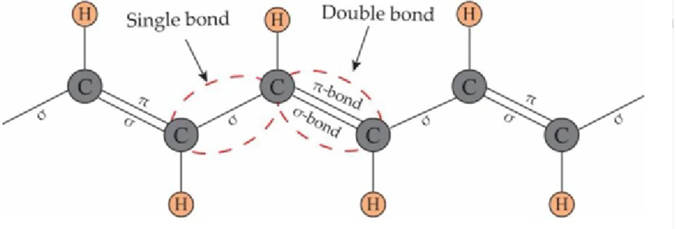
From the perspective of chemists, the electronic characteristic of conductive polymers that favours their wide usage is the presence of conjugated single and double bonds along the polymer skeleton. While the single bond contains a localized strong θ-bond, the double bonds include a localizedθ-bond and a weaker localizedπ-bond.

Figure 2.5: Conductive polymer structure

The electric flow results from the constant transfer ofπ-bonds that are between con-secutive carbon atoms. The resulting eff_{ect will cause electrons in the double bonds to} move along the carbon chain (the pz-orbitals in the chain ofπ-bonds overlap

continu-ously and the electrons in theπ-bonds move along the carbon skeleton). Even though this creates a degree of current flow, it does not justify the widespread usage of conductive polymers. The breakthrough that caused their increased presence and predominance was achieved by Shirakawa, Heeger, and MacDiarmid, discovered that, by applying a halogen dopant would remove an electron from a delocalized bonding arrangement creating a hole. This hole will be filled by a neighboring electron, which will generate another hole on the previous position the electron was at, allowing charge to flow through the polymer chain. This doping eff_{ect can be seen on figure2.6.}

Figure 2.6: Conductive Polymer Conductivity

2.2.2 Data Acquisition Channel

This segment introduces the concept of a data acquisition channel and which tech-nology is necessary for its development. When a system that interfaces with the analog domain, it must be capable of converting signals - analog - coming from sensors to digital format. This interface is accomplished with an ADC - analog-to-digital converter [9] [26]. As the name implies, an analog-to-digital converter is a peripheral that converts analog signals in a defined range to the corresponding digital outputs [20].

Usually, an ADC is considered to have the following components:

• Operational amplifier

• Sample and Hold circuit

• ADC

Operational AmplifierEver since applications started interacting with real world sig-nals, there is a need to use an interface that will act as a medium between the digital and analog domains. This interface is the ADC and it needs another electronic component that can drive it and amplify the source signal to its full analog input range. This component is the operational amplifier - OpAmp. Besides ensuring optimum signal-to-noise ratio (SNR) and spurious-free dynamic range (SFDR), it is also capable of converting signals from single-ended to diff_{erential. Its major drawback is the amount of noise it introduces} on the circuit, since it is an active component. This can, ultimately, degrade conversion performance.

Sample and HoldThe behaviour of a sample-&-hold circuit results from the current flow that charges the capacitor to a voltage equal toVIN throughRADC. Therefore, the

complete circuit consists of an internal charging resistance and a hold capacitor -C_ADC-, bundled together by an electronically operated switch. As soon as the ADC conversion starts, the electronic switch is closed and a charging current flows through the circuit. The measure of how long this switch is closed is called sampling frequency -fADC -, and

the equivalent time period is calculated bytADC=_fADC1 , which can be seen on figure2.7.

Figure 2.8: Sample-and-hold time diagram

Regardless of type, this block must be implemented with the Nyquist-Shannon theo-rem (cfr. Shannon theotheo-rem) in mind, which states that the sampling frequency must be equal, or greater, than twice the carrier’s frequency, in order to eliminate all the frequency components higher than the Nyquist frequency (equation2.1).

fs≥2fc (2.1)

There are two main techniques for analog-to-digital converters: Successive-approximation-register (SAR) and delta-sigma (DelSig).

Successive approximation Register (SAR) ADC

Figure 2.9: SAR ADC

medium-to-high resolution (8-16 bits) and a sample rate of 5 Mega samples per second (Msps). It is also widely used due to its low power consumption and small form factor. Thus, implementations such as pen digitizers and portable/battery-powered instruments systems can benefit from this technique.

Many iterations of the SAR ADC have been developed and implemented. Nevertheless, its fundamental architecture continues to be simple - figure2.9. After holding theVIN

input voltage, it proceeds to compare this value with a reference -V_REF/2, whereV_REF is the voltage provided to the ADC. Whether it is above or below the reference will cause the ADC output to shift between HIGH and LOW logic values, conversely 1 or 0. This is the binary search algorithm. It is executed from the MSB of the N-bit register until it reaches the LSB and, when finished, the N-bit digital word is available in the register.

Delta-Sigma(∆Σ_{) ADC}

Analog Input Delta Sigma Modulator Digital Low-Pass Filter Decimation Filter 1-bit Data Stream Multi-bit Data Output Data

Figure 2.10:∆Σ_{ADC diagram}

Similarly to the SAR ADC, a delta-sigma (DelSig) ADC is capable of converting signals from the analog to the digital domain. Its design consists in approximately three-quarters digital and one-quarter analog.

The conversion process is based in oversampling the input signal over time, so that it can average the output of each sample. Therefore, the sampling rate is several times faster than the digital results at the output ports. In order to succeed with this implementation, the input signal needs to be somewhat slow (DC to several megahertz).

2.3 System-on-Chip

Nowadays chips house severalµ-processors together with components that used to be peripherals. These electronic devices are called System-on-Chip and, as the name sug-gests, these house a CPU and several other components in one chip, such as the DAC, ADC, USB, RAM, among others. With the current rate of technological development, the price of an SoC has been decreasing and their computing power has been increasing. This enables a bigger audience to tinker with the products and, regarding e-noses, allowed students to develop their own electronic nose solutions[11] instead of buying the more expensive commercial options, such as the ones displayed on table2.1.

Table 2.1: Commercially available e-noses [17]

Model Manufacturer Technology

ChemPro100 Environics ion mobility spectrometry Air Quality Module AltraSens 2 MOX sensors

FOX 4000 Alpha-Mos 18 MOX sensors (or QMB/CP)

oNose Illumina fluorescence sensorssbead array

ZNose 7100 Electronic Sensor Technology GC and SAW

This technology is fundamental for the idea of a portable and still aff_{ordable e-nose.} It is a compact integrated circuit designed to govern a specific operation in an embedded system. Due to the increase in integration of components on chips it is possible to develop a data acquisition channel with these since they can sample the sensor input and transmit the data to another device (most frequently a PC) where the identification procedure is executed. Microcontrollers used to be based on one of two methodologies: CISC or RISC. The former stands for complex instruction set computing and the latter means reduced instruction set computing.

Table 2.2: RISC and CISC architectures

CISC RISC

The original microprocessor ISA Redesigned ISA that emerged in the early 1980s

Instructions can take several clock cycles

Single-cycle instructions

Hardware-centric design: the ISA does as much as possible using hardware circuitry

Software-centric design: High-level compilers take on most of the bur-den of coding many software steps from the programmer

Most effi_{cient use of RAM than} RISC

Heavy use of RAM

Complex and variable length in-structions

Simple, standardized instructions

May support microcode (micro-programming where instructions are treated like small programs)

Only one layer of instructions

Large number of instructions Small number of fixed-length in-structions

Compound addressing modes Limited addressing modes

With continuous development of microcontroller technology, it became increasingly diffi_{cult to draw the line that distinguishes between CISC and RISC MCU.}

There are a variety of Microcontrollers available and choosing one comes down to its price, size, peripherals and capabilities. After careful consideration, and with goal a portable, inexpensive and relatively powerful electronic nose, the following IC are good options for the development of an e-nose project:

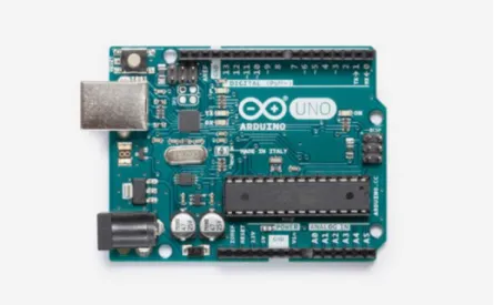
• Arduino Uno from Microchip

• PSoC 5LP from Cypress Semiconductors

• MSP430 from Texas Instruments

Arduino Uno

Based on the ATmega328, by Microchip - implemented with RISC technology - Arduino Uno has 14 digital I/O, operates at 16 MHz (crystal quartz), USB connection, a ICSP header (allows reprogramming of the board without unplugging it from the computer) and a reboot button. It has 328 kB of flash memory, 2 kB of SRAM and 1 kB of EEPROM. The peripherals present on this board are 23 general I/O lines, a RTC (real time counter), three flexible timers/counters with comparators and a PWM, I2C, a 6 channel 10 bits ADC, a Watchdog timer with internal oscillator, a series SPI port and 6 software defined power saving modes.

Figure 2.11: Arduino UNO

Texas Instruments

The MSP430FR2433 device belongs to the MSP430™ family, which is part of the low-cost, with sensory capabilities and measuring MCU. The architecture implementation, as well as the FRAM and the integrated peripherals, with low-power modes and a VQFN (4mm x 4mm) , allow it to operate for large periods of time, even when used for sensing applications. The fast write speeds, flexibility and low-power are a result of the FRAM technology, which is a junction of RAM with the non volatility of Flash.

Figure 2.13: MSP430 board

Freedom Development Board

NXO Semiconductors off_{ers many devices that belong to the MCU universe.} FRDM-KE06Z is part of the freedom development boards microcontrollers and its implementa-tion is based on the Arm® Cortex®-M0+ processor. This microcontroller operates at 48 MHz, with 128 kB of Flash memory, 16 kB of RAM and 256 kB of EEPROM. It supports signals which amplitude varies between 2.7 V and 5.5 V, with -40ºC to 105ºC as working temperatures. As peripherals, it has a 12-bit SAR ADC, a 6-bit DAC, a Power Management Module (PMC), 71 GPIO pins, a programmable CRC (cyclic redundancy check module), a PWM, a series interface, a UART, a I2C and a CAN.

Figure 2.15: FRDM-KE06Z

PSoC 5LP

The PSoC 5LP is a microcontroller developed by Cypress Semiconductors. It comes equipped with a 32-bit ARM Cortex-M3, which operates at a maximum of 80 MHz, as well as with a 24 channel DMA controller. It has 256 kB of flash memory, 64 kB of RAM and 2 kB of EEPROM. This IC contains peripherals that cover both analog and digital domains, such as the Delta-Sigma ADC (8- to 20-bits), comparators, amplifiers, CapSense®support (to a maximum of 62 sensors), 62 GPIO pins. Its digital components include Timers, Counter and a PWM. Regarding communication, the available options are I2C, USB, CAN, among others. Its working temperature range goes from -40ºC to 85ºC and its voltage operating range is between 1.71 V to 5.5 V.

Table 2.3: Microcontroller comparison

Device Clock fre-quency (MHz) GPIO Flash memory (kB) RAM (kB) ADC Other Arduino Uno

16 14 328 2 10-bit USB, PWM, I2C

PSoC 5LP

80 62 256 64 8-20 bits

Delta-Sigma 24-channel DMA controller, Capsense, PWM, Counter, Timer

MSP430 48 17-19 128 16

16-channel 12-bit SAR

6-bits DAC, two 8-bit I,Timer, UART, SPI, I2C, CAN

FRDM-KE06Z

48 71 128 16 12-bits

SAR

6-bits DAC, PWM, UART, CAN, I2C

2.3.1 Identification Software

The last part of the electronic nose system is the algorithm responsible for sample identification. From start, to finish, the sensors are exposed to a chemical sample that induces a change in their baseline response. This is captured by the data acquisition system, which acts as an interface between the analog and digital domains, being also capable of transmitting the data to another device that executes a software, based on an algorithm that can identify the sample origin.

Typically, pattern recognition software is based on classification algorithms such as K-Nearest Neighbour or Artificial Neural Networks [13,22].

• k-NN: k-Nearest Neighbour

In overview, the NN classification algorithm is very intuitive. After having well defined classes, new samples that need to be classified are designated to a class of their nearest neighbours. To increase the effi_{cacy of this method, it became more} useful to consider a certain amount of neighbours - k. Although it is meant to be a generalized way of classifying incoming samples, the k variable can be fine tuned to be responsive and more exact for the classification of certain samples.

• ANN: Artificial Neural Network

This algorithm is based on the behaviour of a human brain. According to [23], it consists on more than 10 billion interconnected neurons responsible for receiving, processing and transmitting information through biochemical reactions. A neuron is made up of 3 parts: dendrite, where the nucleus is located; axon, a fibre that extends from the dendrite and which binds to other neurons through synaptic ter-minals or synapses. Thus, an ANN has artificial neurons as its constituent elements. The synapses of these neurons are represented by a mathematical model where weights represent the eff_{ect of each input and the non-linear characteristic of the} neurons is represented by a transfer function. The neuron pulse is then calculated as the weighted sum of the input signals, obtained by a transfer function. The ability to represent the desired behaviour by the artificial neuron is achieved by adjusting the weights according to the chosen algorithm.

2.4 Electronic nose past implementations

2.4.1 Identification of cannabis-based drugs

Since it became the main producer of cannabis, Morocco struggled against the rise of illegal drugs smuggling in 2003. The main supplier of this substance was the European market, which led to an increase in market turnover of Moroccan cannabis. Also in 2003, this turnover was estimated to be around 12 billion US$.

One method chosen to control this issue was random searches at the border, using trained dogs. Another solution was using specialized equipments, but these were bulky and expensive, thus complicating their widespread use.

Ideally, the solution would involve a device that is portable, aff_{ordable and still able} to execute the systematic process of sampling volatiles released by the person, or their luggage, followed by an analysis. The goal of finding this solution is what led to the development of an electronic nose system that focuses on detecting drugs, especially cannabis derivatives.

The first stage of this portable e-nose consisted on a sensor array with the following devices: TGS 8XX (with XX= 15, 21, 22, 24, 25 and 42). The peculiarity of these sensors is that, even though they have a widespread selectivity for gaseous substance, they still have a degree of affi_{nity towards a specific gas or compound. The idea revolved around} overlapping the sensitivities of each sensor to reach a decision on whether it had traces of cannabis derivatives.

The housing of this e-nose system also contained a relative humidity and a temper-ature sensors, to monitor the conditions of the experiment. Regarding the data acqui-sition segment, it was developed around a microcontroller - PIC16F877 – which was programmed in assembler language, via a serial RS232 communication port. Since the last step of the process revolved around analysing digital data, the incoming sensor signal had to be converted and this was achieved with a 10-bit resolution ADC. On the com-puter side, the data acquisition interface was implemented with LabVIEW©(National Instruments Inc., Austin, TX, USA). The pattern recognition software, responsible for sample identification, was developed using MATALB 7.0.1, from MathWorks Inc.

To test the effi_{cacy of the developed electronic nose, the samples used - snu}ff_tobacco, tobacco leaves, cannabis plants (leaves), cannabis buds and hashish - had to be in line with what was normally found during border searches. These were obtained from the court of justice (Meknes, Morocco).

Figure 2.19: Electrical conductance of TGS842sensor towards exposures to studied drugs[6]

2.4.2 Identification of spoiled beef

Food contamination is a major issue regarding the health of a population. Therefore, it is mandatory to have a process that can constantly examine its condition.

On this study, the goal was to develop a means that could facilitate and accelerate how food analysis is performed, to avoid the consumption of spoiled meat products. For this reason, it is imperative to develop sensing techniques that could prevent situations, like food poisoning. Many of the so far developed methods are limited. They have only been applied in laboratories, are destructive, slow or convenient for field scale use.

The sensing technique implemented on this study considered the metabolic reactions present on food products that produce metabolites in the form of gas, solid and liquids. The micro-organisms would produce these substances and, by studying the headspace of the food product, its possible to determine the quality of a given food product. The sample used to develop this e-nose implementation was 100g of a beef strip loin (M. Longissimus lumborum) from diff_{erent carcasses, obtained after a chilling period of 24} h. Each sample was further divided into two samples of 50g each and packaged in a way that emulated the environment they would have in a grocery store. Besides packaging, also the temperature levels were taken into account to produce an environment similar to that of a grocery store – between 10ºC and 4ºC, where 10ºC was meant to expedite meat spoilage and 4ºC is the typical temperature for meat conservation on grocery stores.

nose (Cyrano Sciences, Pasadena, CA, USA). It consisted of an array with 32 conductive polymer sensors, and each was fine tuned to detect a specific chemical sample. As previ-ously mentioned, the response of a conductive polymer is characterized by a deviation in its conductance and it depends on the level of exposure to the chemical being tested. Af-ter the sensing phase, the output is stored in a format supported by MS Excel for further analysis.

The typical response obtained by the e-nose during this study is showcased on figure 2.20

2.4.3 Healthcare application

The idea of implementing an e-nose in healthcare is related not only with the aff_ordable price point, but also their non-invasiveness when performing a diagnose.

Figure 2.21: Overview of Optical e-nose (the side view of the chamber only shows 2 sensors out of 4)[4]

At the time, this system could perform up to 10 frequency readings per optical detec-tor, which virtually meant that the array system had 33 sensors, sensitive enough to read between 3.1µm and 10µm.

Figure 2.22: Sensor response to CH4 gas with diff_{erent concentrations starts from 2.5} ppm to 100 ppm in two wavelengths 7.88µm (left) & 3.4µm (right).[4]

1ppm, for methane. Since many samples are not simple but a complex mixture of diff_erent substances, it should be able to examine these as well. This system managed to separate complex vapours such as acetone and ethanol.

C

h

a

p

t

3

I m p l e m e n ta t i o n

3.1 Data Acquisition and Transmission

Essentially, the data acquisition segment implementation for this system revolves around selecting the correct sensor for our study and conversion of the sensor’s response to digital format. This interface must allow, among other conditions, conversion of the signal with suffi_{cient resolution to distinguish each specific sample response, possibility} of applying diff_{erent signals to the sensor, a configurable ADC, a reliable transmission} protocol and to have a small form factor.

The sensor type chosen for this electronic nose implementation is theconductive poly-mer. On figures3.1and3.2is displayed the sensor appearance and structure, respectively. By applying a signal to it, a baseline response is obtained and, due to its chemiresistor properties - conductive polymer composites that react diff_{erently, depending on the} sam-ple -, by applying the same signal, a new response is obtained since the conductance was aff_{ected by the gas sample being studied.}

Figure 3.1: Conductive Polymer based sensor

Figure 3.2: Conductive Polymer Structure

Nevertheless, the approach chosen for this dissertation was diff_{erent. At first, a} rect-angular wave is applied to the sensor during 30 seconds, purging the sensor with air and to discover the resulting response, displayed on figure3.3. After, the sensor is exposed to the chemical substance for 30 seconds, achieving saturation around 20 seconds into the exposure period, the moment when the input signal is applied and, at the same time, the sampling procedure starts. It was clear that the sensor behaved exactly like alow-pass fil-ter circuit. While the wave was rising and falling, there is a noticeable curve, resembling a capacitor charging and discharging, obtained at the sensor’s output.

A conductive polymer sensor has a response that resembles the one obtained when measuring the output voltage signal from a capacitor. This behaviour is known as pseudo-capacitance - storage of electricity in an electrochemical capacitor - and is originated by a very fast sequence of reversible faradaic redox processes on the surface of the electrode. Therefore, a rc circuit (figure 3.4) was designed with the goal of fine tuning the data acquisition channel parameters before turning to the sensor – which wasn’t completely characterized - that was going to be used in the final implementation.

Figure 3.4: RC filter schematic and breadboard implementation

The components selected to implement the RC circuit used for testing are described on table 3.1. These where arranged in a way that allowed for a response that smoothly transitioned from rising to steady phase. As a result, resistors 1 and 2 are in parallel and equivalent to 303Ω_{; resistors 4 and 5, also in parallel, are equivalent to 909} Ω_{. This}

translates in a final equivalent resistance of 1.4 kΩ_.

Table 3.1: Components used for the RC circuit

Component Value Capacitor 10µF Resistor 1 510Ω

Resistor 2 750Ω

Resistor 3 200Ω

Resistor 4 10 kΩ

Resistor 5 1 kΩ

Resistor 6 82 kΩ

(Programmable System-on-Chip) by Cypress Semiconductors. Its architecture includes the necessary components that allow both signal generation and data-acquisition - DAC (Digital-to-Analog converter) and ADC (Analog-to-Digital converter). For the acquisition interface, the choice was the Delta-Sigma ADC. This, opposed to the SAR (Successive Approximation Register) ADC, is better at filtering the incoming signal and can convert samples at higher resolution leves, which is ideal for an electronic nose, a system that relies heavily on little diff_{erences of incoming signals.}

There is also the need to use a device with the capability of transferring the acquired data to a second device. It will be responsible for performing the necessary pre-processing on the acquired data, feeding it to a follow-up stage - identification algorithm. Thus, the choice of PSOC 5LP® . This device has several options to execute data transmission be-tween itself and a computer, therefore, becoming the necessary interface bebe-tween sensor and pattern recognition software.

On figure 3.5 it is present the ADC component. It is responsible for sampling the incoming signal response from the sensor. Its configuration revolved around establishing the resolution of each sample and the frequency conversion value. In this case, the goal was to have WORD long samples and a a rate of conversion as high as possible. On figure

Figure 3.5: DelSig ADC component

The DAC component showcased on figure3.7, and its configuration on figure3.8, is used to apply a heaveside wave to the sensor to obtain its response, whether it is exposed to a chemical sample or simply its baseline state. This allows a better study of the response on the frequency domain since it covers the whole spectrum. The three diff_{erent values} for each wave were chosen to test how would the response change according to an bigger or smaller amplitude value. The reason why it is only 3 DAC is because this is a limitation of the microcontroller.

Figure 3.7: DAC component

In such implementations, it is desirable to have some degree of flexibility. In its architecture, the PSoC 5LP® allows a maximum of three active DAC components and one DMA - direct memory access, shown on figure3.9. This last component is crucial for this project because its functionality overcomes one limitation of the device. Before, the number of samples sent to the computer program was limited by the memory size of the microcontroller, since it was responsible for sampling, buff_{ering data and transmitting it.} This meant that the acquisition window was limited and the number of samples acquired was not be enough to feed the identification algorithm.

Figure 3.9: DMA component

Thus, the DMA allows separation of the data acquisition process and its subsequent transmission by allocating two arrays, and while one is being used to store data from the sensor, another is being accessed to send data to the computer. This alternative executes until the desired number of samples is achieved. This iterative process is calledPing-pong DMAand is showcased on figure3.11.

Figure 3.11: Ping Pong DMA schematic

Regarding the data transmission to a computer, this board has several options and the one chosen, mainly due to its speed and throughput is the Universal Serial Bus Full Speed, or USBFS, component. This way, after detecting and acquiring from the sensor, data is sent to a computer that has a program which supports the format sent by the board. Since the ADC was configured to acquire 2-byte samples and the USBFS component could only send values of 1-byte size, each sample acquired is divided in a little endian format and, when received on the computer there is a need convert each value back to 2-Byte format.

Figure 3.13: USBFS component configuration

This way, after configuring each aforementioned component and adding one auxil-iary - Multiplexer, which gives the user options regarding the input signal -, the final circuit designed on the PSoC 5LP® to guarantee a successful data acquisition process is showcased on figure3.14.

3.2 Data Pre-processing

Until this point of the project, every measurement performed required an Oscilloscope, which allowed visualizing the sensor response. Thus, it is necessary to also implement a computer program capable of receiving data sent by the microcontroller and display it afterwards. As mentioned before, the protocol chosen to send data from the PSoC 5LP® is USB. It allows a throughput of 64 bytes of data per transmission, where each sample is BYTE size.

Since each sample acquired by the ADC is a WORD, when sent to a computer, they were converted to Little Endian format. This meant that the software had to be able to receive the data and also convert two consecutive 1-byte long samples in their WORD original representation.

The programming language chosen to develop this segment was Python. This choice was mainly due to its extensive data processing libraries and also because it is open-source.This increases the value of the project since one of the goals is to reduce the cost of development of electronic nose and by using an open sourced language, there is no added cost to it. Also, there are many helpful guides and tutorials which would not exist if it was a closed platform.

In all its entirety, the program can be divided in the following operations:

• Data reception

• Data storage

• Data display

• Data comparison

Figure 3.15: Application start screen: console and GUI

Figure 3.16: Data acquisition GUI window

After finishing the previous step, the user is given the option to either see the acquired sample or any other that might be on a database, composed of previous files saved after their own acquisition processes. Here is where a small degree of preprocessing is applied. At this point, it is desirable that every signal acquired has the same output as a rc filter.

Compared to the approach on [16], this thesis goes further. Instead of only obtaining the voltage output from the sensor, it also takes into account the frequency response to determine the sample origin. This characteristic is calculated from applying the FFT algorithm to the voltage output. This resulting curve is then object of further analysis as to obtain the equation responsible for its graphical representation and this is what will be used to classify each sample, their characteristic transfer function equations.

Since some acquisitions tend to start at an undesired point for this study, it was nec-essary the implementation of a correction algorithm that would only allow the curve that resembled the desired output to be stored in a file that, in the future, will be sent to the identification algorithm.

Figure 3.17: Comparing the output of 6 plots

Figure 3.18: E-nose system database

On figures3.19and3.20is presented the complete e-nose test bench:

3.3 Transfer Function

The main goal of this thesis is the development of a data acquisition channel for an electronic nose. The implementation of this solution revolved around programming a microcontroller that would become the interface between the sensor signal and its digitalization for the computer to process it.

Since the expected response of the sensor, when a step signal is applied to it, is known beforehand to be similar to the equation of a RC circuit, its possible to say that each sample studied will have the transfer function showcased by equation3.1

H(t) = (1−eτt) (3.1)

where,tis the temporal variable andτ is the unique characteristic associated with each response obtained, also called, the time constant.

Therefore, the last step of this project consists in finding the value ofτ. The process to obtain its value is called system identification and it calculates the value ofτ by figuring out what is the relationship between the input - step signal - and the output from the sensor.

To maintain some consistency, the chosen programming language to implement this segment was also Python and the desired tool to achieve it is the Python Control Systems Library.

3.4 Data acquisition channel flowchart

START

END Expose to chemical

compound

Apply input signal to the sensor

Sample the sensor resp onse

Transmit acquired signal

Display signal equation| plot to the user

Save the data

Repeat process?

Y

E

S

NO

C

h

a

p

t

4

R e s u lt s

4.1 Plot results

0 1 2 3 4 5 6

Time [s] 0.0

0.2 0.4 0.6 0.8 1.0

Voltage [V]

RC circuit output

rc 90% 10%

Figure 4.1: RC circuit Python simulation

This output is a representation of the ideal RC step response wave obtained with Python. The values of the resistors and capacitor were established identically as the values they have on the breadboard implementation.

0 1 2 3 4 5 6

time[s] 0.0

0.2 0.4 0.6 0.8

voltage[V]

Signal Plot

connect_170

Figure 4.2: RC circuit breadboard output

4.2 (Breadboard), it can be said that the responses are very similar and, therefore, the data acquisition circuit is working as expected.

Both figures below are a representation of the sensor baseline response - not subject to any chemical compound - when a 1 V dc signal is applied to it. On figure 4.3, it is represented the voltage output and, as it was mentioned on thestate-of-the-art, it is quite similar to the response of a rc circuit. After executing the FFT algorithm mentioned in the Implementation chapter, the obtained response is shown on figure4.4.

0 1 2 3 4 5 6

time[s] 0.0

0.1 0.2 0.3 0.4 0.5 0.6

voltage[V]

Signal Plot

connect_170_baseline

Figure 4.3: Sensor baseline response to a 1 V signal

101 ₁₀0 ₁₀1 ₁₀2 ₁₀3 ₁₀4

40 60 80 100 120

Magnitue Response Plot

connect_170_baseline

The following illustrations showcase the response of the sensor when it’s properties have changed. This change is attributed to the chemical sample being tested as it alters the conductance of the Polymer, resulting in deviations on the curves. While on this state, three diff_{erent signals were applied to it: 1 V, 100 mV and 10 mV. It is noticeable on} the latter two that a heavy influence of noise is present because the signal amplitude is smaller.

0 50000 100000 150000 200000 250000 300000 time[s]

0 10000 20000 30000 40000

voltage[mV]

Signal Plot connect_174

connect_172 connect_171 connect_170_baseline

Figure 4.5: Sensor exposed to chemical compound response to a 1 V signal

101 ₁₀0 ₁₀1 ₁₀2 ₁₀3 ₁₀4

40 60 80 100 120

Magnitue Response Plot

connect_171

0 1 2 3 4 5 6 time[s]

0.00 0.02 0.04 0.06 0.08 0.10

voltage[V]

Signal Plot

connect_177

Figure 4.7: Sensor exposed to chemical compound response to a 100 mV signal

101 ₁₀0 ₁₀1 ₁₀2 ₁₀3 ₁₀4

20 0 20 40 60 80 100

Magnitue Response Plot

connect_177

0 1 2 3 4 5 6 time[s]

0.000 0.002 0.004 0.006 0.008 0.010 0.012 0.014

voltage[V]

Signal Plot

connect_181

Figure 4.9: Sensor exposed to chemical compound response to a 10 mV signal

101 ₁₀0 ₁₀1 ₁₀2 ₁₀3 ₁₀4

40 20 0 20 40 60 80

Magnitue Response Plot

connect_181

The goal of this application is to notice diff_{erences in sensor behaviour according to the} chemical sample being tested. On figure4.11, these deviations are clearly defined. While every curve, besides the baseline, should, ideally, be on top of each other, the deviation is not drastic. On the other hand, there is a clear distinction between the baseline curve and the others, which showcases that the data acquisition channel is capturing, successfully, the diff_{erences in sensor response.}

0 50000 100000 150000 200000 250000 300000

time[s] 0 10000 20000 30000 40000 voltage[mV] Signal Plot connect_174 connect_172 connect_171 connect_170_baseline

Figure 4.11: Sensor output responses compared

101 ₁₀0 ₁₀1 ₁₀2 ₁₀3 ₁₀4

Frequency[Hz] 40 60 80 100 120 Gain[dB] Frequency Plot connect_174 connect_172 connect_171 connect_170_baseline

C

h

a

p

t

5

C o n c l u s i o n a n d F u t u r e Wo r k

5.1 Final Remarks

This implementation of a data acquisition channel for an electronic nose is only pos-sible due to the technology development verified on recent years in fields such as micro controllers, sensors and data processing libraries available for open source programming languages, such as Python. The structure of it is divided in three main blocks: sensor array, electronic board and computer software. The sensor array suff_{ers a deviation from} its normal response to incoming signals based on whether it is being exposed to a fluid or not. After it, the electronic board is capable of sampling this incoming signal and send it to another device with software capable of pre-processing and storing the data. Based on the requirements initially stated for the development of this dissertation, it can be considered successful. Data acquisition and subsequent transmission was achieved with a degree of flexibility that allows further developments on top of this implementation possible. Regarding the final step of identifying between diff_{erent gases, it was was not} possible to achieve this goal.

5.2 Future Developments

[1] K. Arshak, E. Moore, G. M. Lyons, J. Harris, and S. Cliff_{ord. “A review of gas} sensors employed in electronic nose applications.” In: Sensor Review24.2 (2004), pp. 181–198. i s s n: 02602288. d o i: 10 . 1108 / 02602280410525977. u r l: www .

emeraldinsight.com/0260-2288.htm.

[2] H. Debéda, D. Rebière, J. Pistré, and F. Ménill. “Thick film pellistor array with a neural network post-treatment.” In: Sensors and Actuators: B. Chemical27.1-3 (1995), pp. 297–300.i s s n: 09254005.d o i:10.1016/0925-4005(94)01605-H.

[3] C. Di Natale, D. Salimbeni, R. Paolesse, A. Macagnano, and A. D’Amico. “Porphyrins-based opto-electronic nose for volatile compounds detection.” In:Sensors and Actu-ators, B: Chemical65.1 (2000), pp. 220–226.i s s n: 09254005.d o i:

10.1016/S0925-4005(99)00316-0.

[4] S. Esfahani and J. A. Covington. “Low Cost Optical Electronic Nose for Biomedical Applications.” In:Proceedings1.4 (2017), p. 589. i s s n: 2504-3900.d o i: 10.3390/

proceedings1040589. u r l: http://www.mdpi.com/2504-3900/1/4/589.

[5] J. W. Gardner, H. W. Shin, and E. L. Hines. “Electronic nose system to diagnose illness.” In: Sensors and Actuators, B: Chemical 70.1-3 (2000), pp. 19–24. i s s n: 09254005.d o i:10.1016/S0925-4005(00)00548-7.

[6] Z. Haddi, A. Amari, H. Alami, N. El Bari, E. Llobet, and B. Bouchikhi. “A portable electronic nose system for the identification of cannabis-based drugs.” In:Sensors and Actuators, B: Chemical155.2 (2011), pp. 456–463. i s s n: 09254005. d o i: 10.

1016/j.snb.2010.12.047. u r l: http://dx.doi.org/10.1016/j.snb.2010.12.

047.

[7] G. Harsányi. “Polymer films in sensor applications: a review of present uses and future possibilities.” In: Sensor Review20.2 (2000), pp. 98–105. i s s n: 0260-2288.

d o i: 10.1108/02602280010319169. u r l: https://www.emeraldinsight.com/

doi/10.1108/02602280010319169.

[8] D. James, S. M. Scott, Z. Ali, and W. T. O’Hare. “Chemical sensors for electronic nose systems.” In: Microchimica Acta149.1-2 (2005), pp. 1–17. i s s n: 00263672.

[9] X. Jiang, P. Jia, R. Luo, B. Deng, S. Duan, and J. Yan. “A novel electronic nose learn-ing technique based on active learnlearn-ing: EQBC-RBFNN.” In:Sensors and Actuators, B: Chemical249.May (2017), pp. 533–541. i s s n: 09254005.d o i:10.1016/j.snb.

2017.04.072.u r l:http://dx.doi.org/10.1016/j.snb.2017.04.072.

[10] T.-H. Le, Y. Kim, and H. Yoon. “Electrical and Electrochemical Properties of Con-ducting Polymers.” In: Polymers 9.4 (2017), p. 150. i s s n: 2073-4360. d o i: 10 .

3390/polym9040150.u r l:http://www.mdpi.com/2073-4360/9/4/150.

[11] M. Macias Macias, J. E. Agudo, A. Garcia Manso, C. J. avier Garcia Orellana, H. M. anuel Gonzalez Velasco, and R. Gallardo Caballero. “A compact and low cost electronic nose for aroma detection.” In: Sensors (Basel, Switzerland)13.5 (2013), pp. 5528–5541. i s s n: 14248220. d o i:10.3390/s130505528.

[12] A. Manbachi and R. S. Cobbold. “Development and application of piezoelectric materials for ultrasound generation and detection.” In: Ultrasound 19.4 (2011), pp. 187–196. i s s n: 1742271X. d o i: 10.1258/ult.2011.011027. arXiv: arXiv:

1011.1669v3.

[13] S. Panigrahi, S. Balasubramanian, H. Gu, C. Logue, and M. Marchello. “Neural-network-integrated electronic nose system for identification of spoiled beef.” In:

LWT - Food Science and Technology39.2 (2006), pp. 135–145.i s s n: 00236438.d o i:

10.1016/j.lwt.2005.01.002.

[14] T. Pearce, S. Schiff_{man, H. Nagle, and J. Gardner, eds. Handbook of Machine}

Olfac-tion: Electronic Nose Technology. Wiley-VCH, 2002, p. 633. i s b n: 047186109X.

[15] N. A. Rakow and K. S. Suslick. “A colorimetric sensor array\nfor odour visualiza-tion.” In: Nature406.August (2000), pp. 710–713. u r l:http://www.nature.com/

nature/journal/v406/n6797/pdf/406710a0.pdf.

[16] R. T. da Rocha, I. G. R. Gutz, and C. L. do Lago. “A Low-Cost and High-Performance Conductivity Meter.” In: Journal of Chemical Education74.5 (1997), p. 572. i s s n: 0021-9584. d o i: 10.1021/ed074p572. u r l: http://pubs.acs.org/doi/abs/10.

1021/ed074p572.

[17] F. Röck, N. Barsan, and U. Weimar. “Electronic nose: Current status and future trends.” In: Chemical Reviews 108.2 (2008), pp. 705–725. i s s n: 00092665. d o i:

10.1021/cr068121q. u r l: http://pubs3.acs.org/acs/journals/doilookup?

in{\_}doi=10.1021/cr068121q{\%}5Cnhttp://pubs.acs.org/doi/pdf/10.

1021/cr068121q.

[18] M. S. Freund and N. S. Lewis. “A chemically diverse conducting polymer-based "electronic nose".” In: Proceedings of the National Academy of Sciences of the United States of America 92.7 (1995), pp. 2652–2656. i s s n: 0027-8424. d o i: 10.1073/

pnas.92.7.2652. u r l: http://www.pubmedcentral.nih.gov/articlerender.