Fuel and foreign currency derivatives use in the Us airline industry

(1)

A Work Project, presented as part of the requirements for the Award

of a Master’s Degree in Finance from the NOVA School of Business

and Economics.

FUEL AND FOREIGN CURRENCY DERIVATIVES USE IN THE US

AIRLINE INDUSTRY- THE IMPACT ON TOBIN’S Q

FRANCISCO DUARTE FARIA GARCIA DA CONCEIÇÃO

STUDENT 3230

A project carried out in form of “directed research”, under the

supervision of: Professor Fernando Anjos

(2)

Abstract

This thesis examines the use of foreign currency and fuel derivatives by a sample of 26 passenger airlines, between 2000 and 2016. The main goal is to study the impact on Tobin’s Q. Based on previous literature, I investigate if there is a premium associated with using these derivatives, controlling for other variables that might affect Q. The results are not statistically significant but point to a positive premium associated with the use of currency derivatives and a discount for the use of fuel derivatives. These results are consistent with an alternative approach, using ROA, stock returns and revenue growth sensitivity to fuel and currency prices. I also study the likeliness of a firm hedging these risks based on its fundamentals. A negative correlation between jet fuel prices and the price of the US dollar relative to a representative basket of currencies indicates the possible presence of a natural hedge, meaning that losses from high prices in one of the factors may be offset by gains in the other.

(3)

In the past decades many authors have discussed the benefits and drawbacks of risk management by all sorts of firms, and tried to figure out how far a company should go regarding risk mitigation or acceptance. For this, researchers have looked into economic fundamentals, investors’ perceptions, opportunity costs, financing costs, among others. The aim of this paper is to determine how investors value a company that hedges certain risks versus a company that does not, and also, to determine the profile of a company that hedges. The airline industry in the United States will be the subject of this study to avoid having the results driven by industry specific effects. Furthermore, I will look into jet fuel costs and foreign currency movements since these are crucial determinants of costs and revenues, respectively.

Modigliani and Miller argue that the value of a firm is independent of whether or not it hedges some risks: investors are able to hedge on their own so there is no need for firms to do it, and efficient and frictionless markets will price derivatives in a way that would make them irrelevant. However, these propositions require strong assumptions that do not hold most of the time. Friction caused by taxes, irrationality, lack of information and more, lay the ground for possible benefits in managing risk. Géczy et al. (1997), Nance et al. (1993), Mian (1996), and others, argue that risk management can be successful in reducing corporate income taxes, reducing the probability and expected costs of financial distress, preserving cash-flows necessary to carry out important projects and investments.

Jet fuel costs are a large and significant portion of an airline’s expenses and are also one of the most volatile. The price of jet fuel can change almost daily and is different between countries and even between airports within the same country. The primary way airlines tackle this variability is to reflect it in the cost of tickets sold which is similar to what oil companies do with refining margins. The firm’s objective is to maintain a somewhat steady profit margin and so it will increase or decrease the price of its tickets based on the price of fuel. However, increased competition, the surge of low-cost carriers and increased tourism, has made travellers more price sensitive since they now have many options to choose from. This means that airlines are no longer able to reflect as much of the cost as they were before, when travelling was almost exclusive to business passengers and families of high-income classes.

The case for foreign currency is slightly different. An airline based in the United States has almost all of its costs denominated in US dollars – taxes, salaries, fuel, maintenance, etc. On the other hand, carriers interested in attracting foreign costumers or operating international

(5)

routes, will usually offer their tickets in various currencies. This means that they will have to exchange those foreign revenues for US dollars, and this is where the risk lies. If the US dollar depreciates against a foreign currency, then the same amount of that currency is now worth more US dollars. For airlines in general, devaluation is good as they will receive more US dollars for the tickets they sold abroad, while appreciation is not desirable. Since airlines cannot control currency prices, they have to make sure that they are able to charge a price that is competitive for foreign customers and that guarantees the necessary cash-flows, when converted to US dollars.

The theory tested here is that companies that hedge have a higher valuation, all else equal, than companies that do not hedge, based on the findings of Allayannis and Weston (2001) and Carter et al. (2002). Valuation is measured with Tobin’s Q (also referred to as Q or Q ratio), which is a ratio of the market value of a firm to the value of its assets. It is a comparison between investor’s valuation of a company and the value of its assets. If investors have a good perspective on a company, the market value increases and the asset value stays the same, which increases that firm’s Tobin’s Q. This means that if investors value the use of derivatives, then it will have a positive impact on Q. I find that both users of currency derivatives and users of fuel derivatives have lower mean Q’s than non-users. Hedgers, meaning that they use at least one type of derivative, also have lower mean Q’s. When controlling for other drivers of Q, such as size and growth opportunities, I find a non-significant premium ranging between 0.0013 and 0.0646 for the use of currency derivatives. On the contrary, using fuel derivatives reduces Q by 0.0202 approximately. I also conduct an event study for changes in hedging policy. Starting to use fuel derivatives has a positive impact whereas starting to use currency derivatives has a negative impact. Stopping the use of derivatives has a positive impact for both types.

I further investigate the common characteristics that make a firm more likely to use derivatives and find that these differ between users of currency derivatives and users of fuel derivatives. Firms with more leverage, higher return on assets and lower relative levels of Capex are more likely to use currency derivatives but less likely to use fuel derivatives. Also, firms are more likely to use just on type of derivative than both.

Since hedging has the objective to reduce the sensitivity of cash-flows to the underlying that is being hedged, I develop a model, based on the work of Allayannis and Ofek (2001), that measures the sensitivity of revenue growth, return on assets and stock returns towards fuel and currency prices for each airline and test what effect the use of derivatives has on these sensitivities. With this, and by estimating the impact of the sensitivities on Tobin’s Q, I

(6)

indirectly estimate the impact of derivatives on Q. The results are consistent with the previous, where currency derivatives have a positive impact and fuel derivatives a negative one.

Finally, I also look into the historical correlation between fuel prices and an index composed of a basket of currencies against the US dollar. I find that US dollar devaluations are correlated with fuel price increases and vice versa, which indicates the possible presence of a natural hedge, where losses in one may be offset by gains in the other.

Please note that, throughout this paper, I only look into the use of derivatives as a hedging mechanism, and for this reason, when I refer to hedging, I am only referring to using derivatives. Other forms of hedging are not contemplated.

This paper proceeds as follows. Section 2 gives a brief overview of the previous literature regarding corporate hedging and the use of derivatives. Section 3 describes the sample and the hypothesis that guide the research. Section 4 presents the results and methodology. Finally, section 5 concludes.

2. Literature Review

2.1. Corporate Hedging

According to Froot et al. (1993), finance theory is very clear about how firms should implement hedges, but it does not say which risks should be hedged and to what extent they should be hedged – totally or partially? The authors argue that hedging makes sense if the costs of external financing outweigh the costs of using internally generated funds. In this case, hedging ensures that a company can better predict how much money it will generate, allowing it to take advantage of investment opportunities that it might face. The rationale behind hedging is simple: if a firm does not hedge, its cash flows will have higher variations, which will imply higher variations in external financing and investment spending. A cash shortfall will increase the amount of external financing and decrease the amount of investment spending. Furthermore, they find that options allow firms to better control investments and financing than forwards and futures, since they are more flexible, and that if investment opportunities are strongly correlated with cash-flows, companies do not want to hedge.

By looking into the use of three types of derivatives, currency, commodity and interest rate, Mian (1996) tries to prove the integrity of different motives typically associated with corporate hedging. In particular, the author looks into financial distress cost models, tax-based models and scale economies, capital market imperfections and contracting costs. In the end, only

(7)

evidence of economies of scale in hedging is found. For the other factors, there is no evidence of a hedging premium arising from lower contracting costs, lower external financing costs or reduced expected tax liabilities.

Gay and Nam (1998) build on the work of previous literature such as Froot et al. (1993) by looking deeper into how underinvestment determines the use of hedging mechanisms. Specifically, they look into the interaction between investment opportunities and a company’s cash pile, and the correlation between cash flows and investment expenses. The evidence found is in line with previous studies. As in Froot et al. (1993), firms that have a high correlation between cash flows and investment opportunities have a lower tendency to hedge. Firms do tend to hedge more when its cash stocks are smaller, and they face good investment opportunities. As previously stated, external financing is costlier than internally generated funds, so firms with low cash stocks need to better control their cash flows.

Because large, widely-held corporations have stockholders and bondholders who have the ability to construct their own well diversified portfolios, Smith and Stulz (1985) look into these corporations and consider hedging as part of a company’s financing decisions. That is, instead of treating firms as risk-averse as most literature does, the authors consider them to be focused solely in maximizing the value of the firm.

According to their analysis, large corporations can hedge for three reasons: taxes, costs of financial distress and managerial risk aversion. If firms face a convex tax function, that is, when the average effective tax rate increases with the pre-tax income, the benefits from hedging are higher. If the reduction in bankruptcy costs is greater than the costs associated with hedging, large firms might find it beneficial to hedge, even if the bankruptcy costs are very small relative to the firm’s size. Also, since these costs represent real costs for stockholders and bondholders, they might prefer to hedge even if it is costly. Furthermore, since bond covenants are associated with accounting numbers and not economic numbers, corporations will benefit from reducing the volatility of its cash flows to protect themselves against breaching the covenants. As for managers, if part of their compensation is dependent on earnings, as it often is, reasons to hedge differ. For example, if there is a bonus that is only paid if a certain earnings target is reached, managers are not expected to hedge if this reduces earnings. On the other hand, if management has stock options, then they are more likely to hedge given that they are not expected to hold diversified portfolio and so will have an incentive to reduce the variance of the firm’s returns.

(8)

2.2. Fuel Hedging

Carter et al. (2002) serves as an important reference for this study as it focuses on the US airline industry and its practices of fuel hedging. They are successful in finding a relation between jet fuel hedging and firm value, specifically a hedging premium of approximately 12-16% of firm value, in the period 1994-2000. The paper argues that hedging has a positive impact on value since it reduces underinvestment. Carter et al. (2002) chose their sample and object of study for two reasons: firstly, by focusing on a single industry, it is less likely that results are driven by differences in hedging strategies; secondly, because of the historical positive correlation between investment spending and jet fuel costs in the airline industry and the fact that airlines face serious distress costs as evidenced in Pulvino (1999).

Hedging can assist in an airline’s ability to invest since it helps predict future cash-flows, allowing for large investments to take place such as aircraft purchases that have to be planned years ahead. In their analysis, the authors find that airline investment is positively correlated with high fuel prices, meaning that there are more investment opportunities in periods of high fuel costs. Combined with the fact that in these periods industry cash-flows tend to be lower, it shows that hedging is useful in preserving cash-flows for investment, which yields that capital expenditures are more valued in hedgers than non-hedgers.

Carter et al. (2006) find a smaller but positive hedging premium for the period 1992-2003, of approximately 10%. When looking at the interaction between hedging and capital expenditures, they find that increases in the latter, are correlated with a higher hedging premium, which is consistent with the proposition that hedging adds value because it reduces underinvestment.

Carter et al. (2014), while replicating their previous studies for an updated database, also look at how the exposure to jet fuel costs influences the decision to hedge. In particular they find that airlines increase their hedging activity when fuel prices are high, are rising and when the exposure to fuel prices is larger. Moreover, they see that this exposure is higher when fuel prices are high and/or rising. The hedging premium found in previous years is also found in this study, however, it is smaller and does not increase with an airline’s exposure. In fact, they conclude that investors are more likely to value a firm with a consistent hedging program, than a firm that only hedges when its levels of exposure are higher, and fuel prices are also higher and/or rising. This might be a sign that an airline acted too late, by waiting for prices to go up.

(9)

If the hedging program was set up when exposure was lower, the hedging instruments would be highly valued by investors when prices went up, and we would see a higher premium. Cobbs and Wolf (2004), conduct an industry survey to US airlines as of December 31, 2003, to learn what fuel hedging instruments the industry had in place at the time, and relate them to market value. First, they find that there is not a perfect hedging instrument: over-the-counter derivatives are very expensive and limited, and exchange-traded derivatives are not available in the US, so airlines rely on derivatives on commodities that are highly correlated with jet fuel such as heating oil or crude. Then, they find that the optimal strategy is to use different kinds of derivatives, resulting in a dynamic hedging strategy that locks prices when fuel cost is low and caps them when prices rise. Many airline executives have made a case against hedging as they believe it is simply betting against the market, and investors would find that irresponsible. However, previous research has shown that airlines that do hedge have a competitive advantage against those that remain unhedged. From what they have observed with the survey and the airlines’ financials, those that have been more successful have dynamic hedging programs in place, while those airlines that face a high bankruptcy risk, face such a risk because of their high exposure to jet fuel costs.

2.3. Foreign Currency Hedging

Allayannis and Weston (2001) focus on a sample of 720 nonfinancial US firms between 1990 and 1995, and study whether the use of foreign currency derivatives has impact on their Tobin’s Q’s. They separate their sample into firms that have foreign exposure and firms that do not have this exposure, basing this separation on a firm’s amount of foreign sales.

Univariate tests show that the mean and median Q’s of users of currency derivatives are consistently higher than those of non-users, and these results are robust to various controls and time effects. The authors find that, when adjusting for the industry, firms that have foreign exposure show evidence of a premium that ranges from 3.62% to 5.34%. For firms that do not have foreign exposure though, the authors find no evidence of a premium.

Hedging should have a positive benefit in the years where the dollar appreciates since it offers protection against a decrease in the value of foreign denominated sales. On the contrary, firms that hedge in years where the dollar depreciated will probably experience less gains than unhedged firms. Consistently, the authors find that the hedging premium is much larger during the years that the dollar appreciated than when it depreciated. However it is beneficial in both situations.

(10)

The authors perform an event study to examine whether the decision to start or stop hedging has an impact on firm value. They find that firms that begin hedging, show an increase in their Q relative to firms that remain unhedged, while firms that quit hedging show a decrease in their Q relative to firms that remained hedged.

Géczy et al. (1997) investigate why firms use currency derivatives, looking into a large sample of Fortune 500 companies that have potential foreign exposure. They look specifically into research and development (R&D) expenses and short-term liquidity and conclude that firms that have greater growth opportunities and that are more financially constrained are more likely to use this type of derivatives. Also, they find that foreign-denominated debt acts as a substitute for currency derivatives for firms that have a considerable amount of the former, since they did not find a relation between R&D expenses and short-term liquidity, and currency derivatives use. By having foreign-denominate debt, firms can avoid exchanging foreign currency by using it to pay for that debt. The authors also find evidence of economies of scale in costs, since larger firms and firms that use other types of derivatives are more likely to use foreign currency derivatives. The benefits of hedging are the greatest when firms have large foreign exchange-rate exposure.

Allayannis and Ofek (2001) also look into currency derivatives use by a sample of fortune 500 companies, to assess whether these firms use them for hedging or for speculative purposes. They examine the impact of currency derivatives on firm exchange-rate exposure, foreign sales and trade, and also factors such as size and R&D expenses. Exchange-rate exposure decreases with the use of derivatives, meaning that the derivatives serve a hedging purpose. Moreover, foreign sales and trade appear to be very important factors in a firm’s decision to hedge and how much to hedge, while the other factors (size, R&D, market value of assets...) only appear to influence the decision on whether or not to hedge.

Dufey and Srinivasulu (1983) make a case for corporate hedging of foreign exchange risk by rebuffing the main arguments against it, such as Purchasing Power Parity (PPP), Capital Asset Pricing Model (CAPM) and the Modigliani-Miller Theorem. Firstly, several studies have shown that PPP does not hold in short-term horizons and so firms can be exposed to risks if the relative price of inputs and outputs changes. Secondly, even though for CAPM only systematic risk matters, hedging has proved to reduce default risk and bankruptcy costs, so it is important for firms that face such a risk. Lastly, companies have a scale advantage in hedging since they can achieve it less costly than individual investors. Also, asymmetry of information

(11)

does not allow investors to accurately assess a company’s exposure to foreign exchange risk. The authors also disagree with the assumption of risk-neutrality, saying that investors are usually risk-averse and if hedging means they will bear less risk, then it is seen as a source of value.

3. Research Design 3.1. Sample choice

This research focuses on the US airline industry for two main reasons. First, by focusing on a specific industry, I am able to isolate the effects of hedging without worrying that the results might be driven by different hedging strategies. The second reason is that, according to Pulvino (1998), the airline industry is characterized for large investment spending and significant distress costs, making it an industry where risk management plays a very important role. Previous literature has been fairly unanimous about the motives and benefits of hedging, regardless of industry and geography. Despite some different results, all authors present similar logical arguments for derivatives use in risk management. My intention is to build up on past work and present a different view on the relationship between hedging and value. To the extent of my knowledge, there has not been a study on the impact of foreign currency derivatives on airlines and most studies on fuel hedging are rather outdated. The aim of this research is not only to update the literature, but also to add a different perspective.

This paper provides an extensive and thorough analysis of derivatives usage and firm value by contemplating different dimensions of this relation: the direct effect the use of derivatives has on firm value; the reasons behind using derivatives; the effect that derivatives have on firms’ sensitivity to fuel and currency prices and how that affects firm value; and the relation between fuel and currency prices.

3.2. Hypothesis

The hypothesis that will be tested are the following:

First hypothesis: Based on the findings of Carter et al. (2002) and Allayannis and Weston

(2001), I will test if firms that use derivatives as a hedging instrument have a higher Q. I expect to find a positive relationship that would mean that hedging adds value.

(12)

Second hypothesis: I will test if the findings of Géczy et al. (1997) and Mian (1996) hold for

our sample. Specifically, I expect that larger firms, with more investment opportunities and high levels of leverage, are more likely to hedge.

Third hypothesis: Based on the analysis performed by Allayannis and Weston (2001), I will

analyse the impact that the decision to start or stop a hedging strategy has on the Q-ratio. I expect a positive impact when a firm implements a hedging strategy and a negative impact if it quits such strategy.

Fourth hypothesis: Inspired by the work of Allayannis and Ofek (2001), I will see if a firm’s

sensitivity to movements in fuel and currency prices decreases with the use of derivatives and if a decrease in such sensitivity has a positive effect in Tobin’s Q.

Fifth hypothesis: I will also look at the historical correlation between fuel prices and currency

movements, and see if there is evidence of the presence of a natural hedge. 3.3. Data

For the sample, I started with all United States listed airlines (defined as firms with SIC codes 4512 and 4513) with annual data available on Compustat for the years between 2000 and 2016. I then excluded non-US firms and all-cargo airlines since these have a very different business model, ending up with 26 firms and 283 firm-year observations.

The data regarding the use of fuel or foreign currency derivatives was extracted manually from the airlines’ 10-k reports available on the Securities and Exchange Commission database, EDGAR. It is considered that a company has used derivatives in a specific year if it is stated in the report that the company has purchased or exercised derivatives in that year, with the sole purpose of hedging.

As a measure of jet fuel and currency prices, data from two indices was retrieved from Bloomberg:

• the Dollar Index Spot (DXY) which is a measure of the value of the US dollar against a basket of foreign currencies: the value was set at a base value of 100 when the index was created (1973). A depreciation of the dollar means that the value of the index went down and vice versa;

• and the New York Harbour 54-grade Jet Fuel Spot market price (JETINYPR): price per gallon in US dollars.

(13)

Table 1 - Summary Statistics All firms

No. of

Obs. Mean Std. Dev. Median

10th percentile 90th percentile Sample: Total Assets 284 9 041.05 12 690.10 2 915.600 256.407 26 313.10 Total Liabilities 284 8 263.72 122 77.29 2 230.15 163.64 29 302.20 Total Revenues 284 7 302.59 10 076.07 2 312.43 441.385 20 165.20 Market Value 284 3 283.06 6 634.61 904.173 60.81 8 792.02 Derivatives: Foreign currency derivatives 284 0.16 0.37 0.00 0.00 1.00 Fuel derivatives 284 0.62 0.49 1.00 0.00 1.00 Tobin's Q 284 1.44 7.42 0.67 0.37 1.57 Controls: CAPEX-to-Sales 283 0.11 0.13 0.07 0.02 0.21 Long-term Debt-to-Assets 284 0.30 0.18 0.30 0.03 0.53 ROA 284 -0.08 1.19 0.02 -0.12 0.11 Dividend dummy 284 0.29 0.45 0.00 0.00 1.00

Passenger Load Factor 283 74.27 11.64 77.30 58.94 84.58

This table presents summary statistics for the sample of US airlines available on Compustat between 2000 and 2016. Foreign currency derivatives and fuel derivatives are dummy variables that equal one if the firm reports using that type of derivative in its 10k annual report. Tobin's Q is the market value of assets divided by the replacement cost of assets. To calculate it, I follow the approach of Chung and Pruitt (1994). The values for Total Assets, Total Liabilities, Total Revenues and Market Value are presented in millions of US dollars. The values for Capex-to-Sales, Long-term Debt-to-Assets and ROA are presented as a ratio. The dividend dummy is equal to one if the firm distributed dividends that year. Passenger Load Factor is presented in percentage points.

Tobin’s Q was chosen as the measure for a company’s value. The Q-ratio is computed by dividing a firm’s market value by the replacement cost of its assets. In theory, it measures the relative valuation given by investors to a company. A high Q means that the company is trading at a value higher than the value of its assets, which suggests investors are confident in that company’s future success.

The methodology used to compute the ratio is the one developed by Chung and Pruitt (1994), both for its simplicity and easiness to collect the data, since it is available in Compustat: the market value is the sum of the market value of equity, the liquidating value of preferred shares, short-term liabilities net of short-term assets and the book value of long-term debt; this is then divided by the book value of total assets. Chung and Pruitt (1994) find that their measure of Q has a high degree of correlation with more complex calculations, therefore concluding that their methodology is accurate.

(14)

To measure the use of derivatives, binary variables are used for each type of derivative in a specific year, which means that the variable for a specific derivative is equal to one if the firm used derivatives in a given year and zero if it did not.

Finally, to better isolate the effect of derivatives, it is necessary to include a set of control variables that could have an impact on the Q-ratio:

Size: As evidenced in previous studies, larger firms are more likely to use derivatives, mainly

because of the high costs of hedging, but also given the larger geographic diversification these firms usually present. For this reason, I include the natural log of total assets to control for the firm’s size.

Dividends: The relationship between firm value and cash dividends is not clear. On the one

hand, paying dividends shows investors that the company’s finances are in good shape and attracts investors that are interested in dividend-paying companies. On the other hand, paying dividends may signal that the company is struggling to find profitable investments to pursue. Also, companies that are less likely to be capital constrained may end up investing in low NPV projects. For this matter, I include a dividend dummy which is equal to one if the company paid a dividend in that year and zero otherwise.

Leverage: Since firms usually hedge as a way to better manage their future cash-flows,

highly-leveraged firms have a higher incentive to do so, in order to mitigate the risk of financial distress. Long-term debt relative to total assets is used to measure the degree of financial leverage of the firms.

Profitability: For profitability, I use the return on assets since it represents how effectively a

company is using its assets to generate money.

Investments: A company’s main investments are usually capital expenditures (CAPEX) and

R&D. Companies that have larger investment opportunities should have a higher incentive to hedge some of their risks, and thus be able to pursue such opportunities. Given that the majority of values for R&D is missing, I use the ratio of CAPEX to revenues as the measure for investment opportunities and investment growth of a company.

Passenger Load Factor: It is an industry-specific measure of operational efficiency. Although

it should not be used as a measure for profitability since it does not say how much passengers payed for the flight, it can be used to check how well an airline manages its routes, aircraft, and attracts costumers, which is valued by those investing in the aviation business.

(15)

Time Effects: Year dummies are used to control for time effects. These are not reported in the

results.

4. Results and Discussion 4.1. First Hypothesis

To study the impact of using foreign currency derivatives and fuel derivatives on a firm’s Tobin’s Q, I will start by performing univariate tests to look for differences between the sub-sample that does not use derivatives and the sub-sub-sample that does. After this, I will regress the derivatives dummies and the control variables on the Q-ratio and see if there is evidence of a premium, and if so, what is the size of such premium.

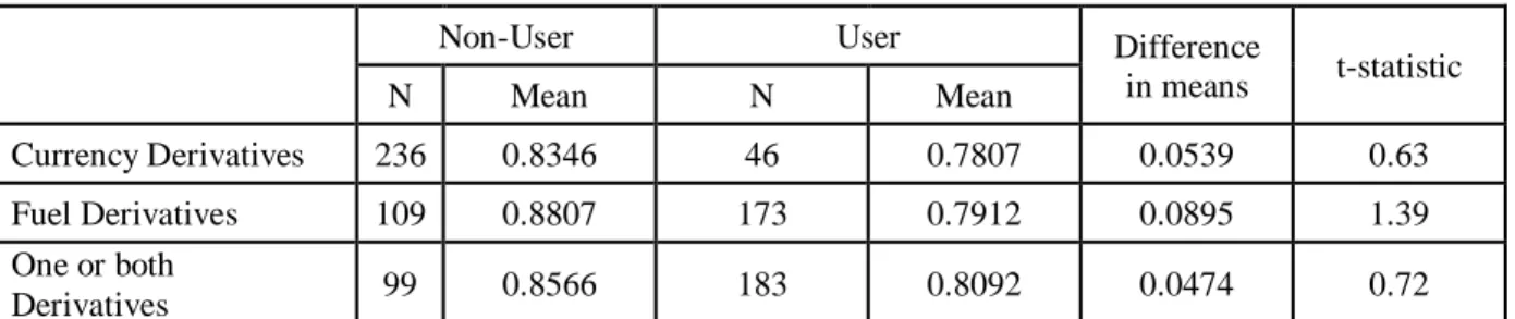
Table 2 presents the results for a univariate test on the use derivatives, separating the type of derivative. Contrary to our expectations, the mean Q for the firms that hedge appears to be lower for both types of derivatives than the mean Q of firms that do not hedge. Statistically, the difference is not significant and by separating the types of derivatives, I do not know if a firm that does not use fuel derivatives for instance, is using foreign currency derivatives. I test for the difference in means between hedgers (of any kind) and non-hedgers, and the results are consistent with the previous ones, where firms that do not hedge have a slightly higher value for Q, with the difference not being statistically significant once more.

Table 2 - Univariate tests

Non-User User _Difference

in means t-statistic N Mean N Mean Currency Derivatives 236 0.8346 46 0.7807 0.0539 0.63 Fuel Derivatives 109 0.8807 173 0.7912 0.0895 1.39 One or both Derivatives 99 0.8566 183 0.8092 0.0474 0.72

This table presents three different univariate tests for the difference in the mean Q. Foreign currency derivatives and fuel derivatives are dummy variables that equal one if the firm reports using that type of derivative in its 10k annual report. Tobin's Q is the market value of assets divided by its the replacement cost of assets. To calculate it, I follow the approach of Chung and Pruitt (1994).

If I do not control for other variables that could have on impact on Q, our results may be biased, and so a more complete analysis should yield more solid results.

𝑇𝑄_𝑖,𝑡 = 𝛼 + 𝛽₁𝐶𝑢𝑟𝑟𝑒𝑛𝑐𝑦 𝐷𝑒𝑟𝑖𝑣𝑎𝑡𝑖𝑣𝑒𝑠_𝑖,𝑡+ 𝛽₂𝐹𝑢𝑒𝑙 𝐷𝑒𝑟𝑖𝑣𝑎𝑡𝑖𝑣𝑒𝑠_𝑖,𝑡 + 𝛽_𝑗𝐶𝑜𝑛𝑡𝑟𝑜𝑙 𝑣𝑎𝑟𝑖𝑎𝑏𝑙𝑒𝑠_𝑖,𝑡+ 𝑌𝑒𝑎𝑟 𝑑𝑢𝑚𝑚𝑖𝑒𝑠 + 𝜀

(16)

I use the control variables listed in section 3.3. and perform regressions using three different models: a pooled OLS model, a fixed-effects model and a random-effects model. Results for these regressions are presented in table 3.

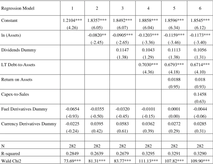
The pooled OLS regression shows positive, yet non-significant, coefficients for both the foreign currency derivatives dummy and the fuel derivatives dummy. The coefficients indicate that users of foreign currency derivatives have a Q that is approximately 0.0013 higher than non-users and for fuel derivatives, there is a premium of 0.0552. These values can also be interpreted as a percentage of the firm’s book value of total assets, since the latter is the denominator in the calculation of the Tobin’s Q. That is, a premium of 0.0552, is the same as a market value premium corresponding to 5.52% of the firm’s total assets. All control variables are statistically significant, with the exception of CAPEX-to-Sales, and present the expected sign. The log of total assets is the only one with a negative sign, while all the others have a positive impact on Q.

Both the fixed-effects model and the random-effects model show similar results between each other, but slightly different from the results of the pooled OLS model. For instance, the coefficient for the use of fuel derivatives becomes negative, while the coefficient for foreign currency derivatives remains positive. In particular, the fixed-effects model shows that the use of fuel derivatives decreases the value of Q by 0.0533 or market value by 5.33% of the firm’s asset value. For foreign currency derivatives there is a premium of 0.0646 (6.46%) which is substantially higher than the premium found with the pooled OLS model. Please note that these coefficients are not statistically significant. As for the control variables, only the log of total assets and the long-term debt-to-assets coefficients are significant with the signs being consistent to what was expected. CAPEX-to-sales presents a negative sign in this model, contrary to what was expected.

The effect of using fuel derivatives, according to the random-effects model is again negative, decreasing Q by 0.0202, and the premium for foreign currency derivatives use is 0.0459. The control variables yield similar results to the fixed-effects model: the log of assets has a negative impact and the long-term debt-to-assets ratio has a positive impact. All the other variables are not significant, but they show the predicted signs.

(17)

Table 3 - Derivatives and Firm Value

Regression Model Pooled OLS Fixed-Effects Random-Effects

Constant 1.2104*** 2.4518*** 1.6740*** (4.26) (3.98) (4.30) ln (Assets) -0.1416*** -0.1903*** -0.1380*** (-5.97) (-2.85) (-3.43) Dividends Dummy 0.2104*** 0.0738 0.0979 (3.02) (0.85) (1.20) LT Debt-to-Assets 0.4236** 0.7739*** 0.6916*** (2.49) (4.60) (4.24) Return on Assets 0.0419* 0.0190 0.0203 (1.71) (0.98) (1.05) CAPEX-to-Sales 0.3559 -0.0675 0.0882 (1.45) (-0.28) (0.38)

Passenger Load Factor 0.0120*** 0.0002 0.0044

(3.43) (0.04) (1.00)

Fuel Derivatives Dummy 0.0552 -0.0533 -0.0202

(0.79) (-0.74) (-0.29)

Currency Derivatives Dummy 0.0013 0.0646 0.0459

(0.02) (0.66) (-0.49) N 282 282 282 R-squared 0.2849 0.1299 0.1985 F-statistic 4.27*** 4.97*** Wald Chi2 114.80***

This table presents the results for pooled OLS, Fixed-effects and Random-effects regressions. The dependent variable is Tobin's Q which is the market value of assets divided by the replacement cost of assets, following the approach of Chung and Pruitt (1994). Currency derivatives dummy and fuel derivatives dummy are variables that equal one if the firm reports using that type of derivative in its 10k annual report. ln (Assets) in the natural logarithm of total assets. Dividends dummy equals one if the firm distributed dividends that year. LT Debt-to-Assets is the ratio of long-term debt to total assets. Return on assets is the ratio of net income to assets. Capex-to-Sales is the ratio of capital expenditures to total sales. Passenger Load Factor is the average percentage of seats airlines are able to sell per flight. Regressions also include year dummies which are not reported. T-statistics are presented between parenthesis. ***, **, * denote significance at the 1%, 5% and 10% levels, respectively.

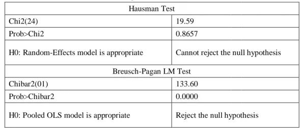
In order to assess the statistical coherency of each model, two test are performed to check which model is more appropriate, according to the data. Specifically, I perform the Hausman test and the Breusch-Pagan LM test. Results are presented in table 4. The Hausman test, tests the null hypothesis that both the random and the fixed effects models yield similar estimates, by estimating and comparing both regressions. The result says that the null hypothesis cannot be rejected, meaning that there is no statistically significant difference between these models. The Breusch-Pagan LM test is used to check which model is statistically better, the pooled OLS or

(18)

the random-effects. The null hypothesis that the variance of the random-effects is zero is rejected and thus the random-effects model is more appropriate than the pooled OLS model.

Table 4 - Hausman and Breusch-Pagan LM tests Hausman Test

Chi2(24) 19.59

Prob>Chi2 0.8657

H0: Random-Effects model is appropriate Cannot reject the null hypothesis

Breusch-Pagan LM Test

Chibar2(01) 133.60

Prob>Chibar2 0.0000

H0: Pooled OLS model is appropriate Reject the null hypothesis

This table presents the Hausman and Breusch-Pagan LM tests for the regressions of table X. The Hausman test compares the consistency of the effects and the fixed-effects estimators. The Breusch-Pagan LM tests if the variance of the random-effects is zero.

4.2. Second Hypothesis

For investors, the decision to hedge and the reasons for it, may be as important as hedging itself. For example, if a firm is more likely to use derivatives when it is capital constrained, investors might want to avoid such a company, and will stay clear of companies that use derivatives. On the other hand, investors might also look for financially constrained companies, if they value the use of derivatives and want exposure to it. The main point is that investors will look into a firm’s use of derivatives, and use it as a proxy for financial stability, profitability and so on, based on the reasons they believe are behind the decision to hedge currency and energy risks.

On this analysis, I look into the probability of using derivatives based on the firm’s characteristics, using both a Logit and a Probit model. Table 5 presents the results for both models, separated by fuel derivatives (panel A) and currency derivatives (panel B).

Starting with fuel derivatives, the size of a firm measured by its assets has a positive influence on the likeliness of using fuel derivatives. CAPEX-to-Sales and the Passenger Load Factor are the other two variables that also have a positive influence. For the results from the regressions, we can only interpret the sign of the coefficient and see if the effect is positive (more probability) or negative (less probability) and its relative impact compared to the other coefficients. However, the marginal effects study lets us draw conclusions from the specific

(19)

Table 5 - Logit and Probit models

Panel A Fuel Derivatives

Logit Probit

Regression Marginal Effect Regression Marginal Effect

Constant -6.6333*** -3.8083*** (-5.42) (-5.66) ln (Assets) 0.6992*** 0.1563*** 0.3941*** 0.1450*** (5.19) (5.22) (5.37) (5.40) Dividends Dummy -1.2751*** -0.2973*** -0.7073*** -0.2682*** (-3.45) (-3.50) (-3.38) (-3.40) LT Debt-to-Assets -3.3911*** -0.7580*** -1.9477*** -0.7168*** (-3.64) (-3.61) (-3.68) (-3.66) Return on Assets -1.4924 -0.3336 -0.8462 -0.3114* (-1.57) (-1.63) (-1.62) (-1.66) CAPEX-to-Sales 1.0934 0.2444 0.5813 0.2139 (0.97) (0.97) (0.85) (0.85)

Passenger Load Factor 0.0402** 0.0090** 0.0240** 0.0088**

(2.20) (2.17) (2.23) (2.21)

Currency Derivatives dummy -0.1693 -0.0385 -0.0907 -0.0338

(-0.37) (-0.36) (-0.34) (-0.34)

N 282 282

LR Chi2 94.31*** 93.32***

Panel B Currency Derivatives

Logit Probit

Regression Marginal Effect Regression Marginal Effect

Constant -12.2644*** -7.0010*** (-3.78) (-4.00) ln (Assets) 0.8740*** 0.0611*** 0.4841*** 0.0700*** (4.79) (3.88) (4.99) (4.17) Dividends Dummy -0.1464 -0.0100 -0.0864 -0.0122 (-0.34) (-0.34) (-0.36) (-0.37) LT Debt-to-Assets 1.5067 0.1053 0.7339 0.1061 (1.02) (1.08) (0.92) (0.96) Return on Assets 0.0495 0.0035 0.0342 0.0049 (0.12) (0.12) (0.15) (0.15) CAPEX-to-Sales -1.2347 -0.0863 -0.6866 -0.0993 (-0.61) (-0.60) (-0.63) (-0.61)

Passenger Load Factor 0.0355 0.0025 0.0229 0.0033

(0.93) (1.01) (1.12) (1.25)

Fuel Derivatives dummy -0.1070 -0.0076 -0.1122 -0.0165

(-0.22) (-0.21) (-0.41) (-0.40)

N 282 282

LR Chi2 59.73*** 60.34***

This table presents the results for logit and probit regressions, separately for fuel derivatives (panel A) and foreign currency derivatives (panel B). The dependent variable is the dummy variable for the fuel derivatives (panel A) and foreign currency derivatives (panel B). ln (Assets) is the natural logarithm of total assets. Dividends Dummy equals one if the firm distributed dividends that year. LT Debt-to-Assets is the ratio of long-term debt to total assets. Return on Assets is the ratio of net income to assets. Capex-to-Sales is the ratio of capital expenditures to total sales. Passenger Load Factor is the average percentage of seats airlines are able to sell per flight. T-statistics are presented between parenthesis. ***, **, * denote significance at the 1%, 5% and 10% levels, respectively.

(20)

value. For example, an increase of one percentage point in the Passenger Load Factor, increases the likeliness of using fuel derivatives by 0.9% (0.88%), on average, according to the logit (probit) model. The coefficient with the largest impact is the Long-term Debt-to-Assets, where a one unit increase in this ratio, decreases the probability by approximately 76% (72%). This goes against the initial prediction that firms that are highly leveraged have a higher incentive to use derivatives in order to better manage their cash-flows. However, Rampini and Viswanathan (2010) develop a model that connects firm financing with risk management. Since both imply payments in the future, then more constrained firms, and with lower cash flows, will give preference to financing and will not hedge. I also find a negative relationship between the Return on Assets and the probability that the firm is using fuel derivatives. This means that a firm that generates more money relative to its assets is less likely to be using fuel derivatives – a decrease of 0.33% (0.31%) for each one percentage point increase in ROA. The use of currency derivatives also decreases the probability of using fuel derivatives, meaning that a firm is more likely to use one type of derivative than to use both. In the end, we see that bigger firms, with lower leverage and higher load factor values, and that do not distribute dividends are more likely to be using fuel derivatives.

The models for the use of currency derivatives are statistically less powerful. The only significant coefficient is the natural logarithm of assets and it has a positive impact. The overall results of these models yield different results relative to the models for fuel derivatives, which means that the reasoning behind using each type of derivative is different. Highly leveraged firms are now more likely to be users of currency derivatives and the same goes for more profitable (high ROA) firms. CAPEX-to-sales, which measures investment growth or investment opportunities, produces a negative impact – a firm with a higher ratio of capital expenditures to sales, is less likely to be using currency derivatives. The coefficient for fuel derivatives is consistent with the previous model, again meaning that the use of fuel derivatives decreases the probability that the airline is also using foreign currency derivatives.

The use of fuel derivatives has the objective of hedging fuel cost while the use of foreign currency derivatives serves mainly to hedge the exchange risk of foreign revenues. Thus, each derivative is used to hedge two different types of cash-flows – costs and revenues. The different purpose of these derivatives might provide a reasoning for the different outcomes of the models described above. When looking at Long-term Debt-to-Assets for example, we see that a firm that has a higher level of financial leverage, is more likely to hedge its foreign revenues, but less likely to hedge its fuel risk. In other words, the firm appears to be more focused in

(21)

controlling its cash inflows than its outflows (through derivatives). Although I have argued that, based on previous literature, hedging adds more value when a firm has a greater need to control its cash-flows, fuel hedging by itself is costly and rather risky. The results seem to indicate that highly leveraged firms prefer to stay clear of fuel hedges and face the risks of fuel prices instead. Firms with higher ROA’s will more likely be using currency derivatives, and less likely fuel derivatives. On the contrary, larger investments in CAPEX relative to a firm’s sales, indicate that the probability of using fuel derivatives is higher, and currency derivatives lower.

It is not possible to validate the second hypothesis, because the profile of a hedger appears to change with the type of hedging that the firm is engaged in. An investor must look into the specific types of derivatives each firm is using if it intends to draw conclusions about the firm’s intentions behind such behaviour.

4.3. Third Hypothesis

If hedging is responsible for a higher level of Q, than that difference should arise when a company starts a hedging policy or when it quits such policy. In this subsection I will investigate whether this is true for the firms in our sample by performing an event study. I follow the approach of Allayannis and Weston (2001) and classify the firms into four categories: HH if a firm hedged in the current and previous period; NN if it did not hedge in this period or the period before; HN if it quit hedging in this period; NH if it started hedging in this period. After this, I regress the one-year change in the value of Q on these four dummy variables, including also the one-year change in the values of the control variables used in 4.1.

∆𝑇𝑄_𝑖,𝑡 = 𝛼 + 𝛽₁𝐻𝐻_𝑖,𝑡+ 𝛽₂𝐻𝑁_𝑖,𝑡+ 𝛽₃𝑁𝑁_𝑖,𝑡+ 𝛽₄𝑁𝐻_𝑖,𝑡+ 𝛽_𝑗∆𝐶𝑜𝑛𝑡𝑟𝑜𝑙 𝑣𝑎𝑟𝑖𝑎𝑏𝑙𝑒𝑠_𝑖,𝑡 + 𝑌𝑒𝑎𝑟 𝑑𝑢𝑚𝑚𝑖𝑒𝑠 + 𝜀

I expect the coefficient of NH, start hedging, to be positive and larger than the coefficient for NN, meaning that the value of Q of a firm that starts hedging is greater, all else equal, than the one of a firm that remains unhedged. Correspondingly, a firm that remains hedged should have a higher Q compared to a firm that quits hedging – the coefficient of HH should be bigger than the one of HN.

As we can see in table 6, results are contrary to what was expected. A firm that starts hedging has a lower Q, all else equal, than a firm that remains unhedged, and a firm that stops hedging

(22)

N β HH 153 0.1251 Test H0: HH = HN (0.09) HN 14 0.6657 F(1, 236) 0.16 (0.35) Prob>F 0.6894 NN 75 0.5644 Test H0: NH = NN (0.39) NH 14 0.4349 F(1, 236) 0.01 (0.24) Prob>F 0.9252

This table presents the results from an event study on how changes in a firm's hedging policies affect its value. The dependent variable is the one-year change in the value of Tobin's Q. HH is equal to one if a firm hedged in the current and previous period; NN is equal to one if it did not hedge in this period or the period before; HN is equal to one if it quit hedging in this period; NH is equal to one if it started hedging in this period. The regression also includes a regressor for the one-year change in the values of ln (Assets), Dividends Dummy, LT Debt-to-Assets, ROA, CAPEX-to-Sales and Passenger Load Factor, which is not reported. Year dummies are also included but are not reported.

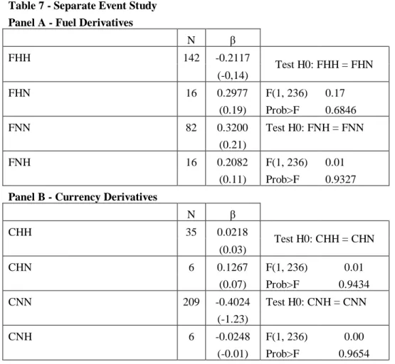
also has a considerably higher Q than the firm that remains hedging. The differences are approximately 0.1295 and 0.5406, respectively. However, since these differences are not statistically significant, we cannot conclude that there is evidence of a hedging discount. In the previous section we saw that the characteristics of firms are different considering which types of derivatives they use, since the objective behind using each type is different. For this reason, it is important to perform this event study separating between fuel derivatives and currency derivatives. The results for this regressions are presented in table 7. In panel A we have the results for fuel derivatives, which are similar, compared with the previous analysis. A firm that quits a fuel hedging strategy, experiences an increase in Q of 0.5094 points relative to a firm that remained hedging. As for a firm that does not hedge, its Q is 0.1118 points higher than a firm’s Q that began hedging. These differences are not statistically significant, but they are again contrary to what was expected. Particularly, the negative sign of the coefficient of HH, means that a firm that used derivatives both in the previous period and in the current period, is trading at a discount compared to a firm that has not hedged either period. This was also the result of 4.1. where the coefficient for the fuel derivatives dummy had a negative sign in the random and fixed-effect regressions. The results for the foreign currency derivatives (panel B) are slightly different. Whilst we still see that a firm that hedges has a lower Q than a firm that quit hedging, a firm that starts hedging now presents a higher Q than a firm that remains unhedged. Interestingly, both signs of the coefficients are negative, but there is a net positive premium of approximately 0.3776 for a firm that starts using currency derivatives.

(23)

None of these models has yielded statistically significant results, which means that it is not possible to confirm the third hypothesis. On the contrary, the results point in the opposite direction, meaning that the decision to remain hedged or to start hedging affects Tobin’ Q negatively.

Table 7 - Separate Event Study Panel A - Fuel Derivatives

N β FHH 142 -0.2117 Test H0: FHH = FHN (-0,14) FHN 16 0.2977 F(1, 236) 0.17 (0.19) Prob>F 0.6846 FNN 82 0.3200 Test H0: FNH = FNN (0.21) FNH 16 0.2082 F(1, 236) 0.01 (0.11) Prob>F 0.9327

Panel B - Currency Derivatives

N β CHH 35 0.0218 Test H0: CHH = CHN (0.03) CHN 6 0.1267 F(1, 236) 0.01 (0.07) Prob>F 0.9434 CNN 209 -0.4024 Test H0: CNH = CNN (-1.23) CNH 6 -0.0248 F(1, 236) 0.00 (-0.01) Prob>F 0.9654

This table presents the results from an event study on how changes in a firm's hedging policies affect its value, separating both types of derivatives. The dependent variable is the one-year change in the value of Tobin's Q. HH is equal to one if a firm hedged in the current and previous period; NN is equal to one if it did not hedge in this period or the period before; HN is equal to one if it quit hedging in this period; NH is equal to one if it started hedging in this period. The regression also includes a regressor for the one-year change in the values of ln (Assets), Dividends Dummy, LT Debt-to-Assets, ROA, CAPEX-to-Sales and Passenger Load Factor, which is not reported. Year dummies are also included but are not reported.

4.4. Fourth Hypothesis

Allayannis and Ofek (2001) develop a model for the sensitivity of stock returns to movements in currency prices by calculating a beta between the stock’s return and the return on an exchange rate index, measured in US dollars per unit of foreign currency. With this model as a starting point, I will try to develop an alternative measure of the impact the use of derivatives has on Tobin’s Q.

(24)

I start by calculating each firm’s sensitivity (beta) to movements in the price of Jet Fuel and US dollars by using the two indices described in 3.1.: DXY and JETINYPR. For this, I will not only use stock returns, but also the Return on Assets and the Growth in Revenues. I regress these three measure on DXY and JETINYPR, individually for each airline.

𝑆𝑡𝑜𝑐𝑘𝑅𝑒𝑡_𝑖,𝑡/𝑅𝑂𝐴_𝑖,𝑡 /𝑅𝑒𝑣𝑒𝑛𝑢𝑒𝐺𝑟_𝑖,𝑡 = 𝛼 + 𝛽₁𝐷𝑋𝑌_𝑖,𝑡+ 𝛽₂𝐽𝐸𝑇𝐼𝑁𝑌𝑃𝑅_𝑖,𝑡+ 𝜀

After calculating the different betas, I will see if they decrease or increase with the use of derivatives.

𝛽1𝐷𝑋𝑌(𝑅𝑂𝐴 𝑆𝑡𝑜𝑐𝑘𝑅𝑒𝑡⁄ ⁄𝑅𝑒𝑣𝑒𝑛𝑢𝑒𝐺𝑅)𝑖,𝑡 = 𝛼 + 𝛽1𝐶𝑢𝑟𝑟𝑒𝑛𝑐𝑦 𝐷𝑒𝑟𝑖𝑣𝑎𝑡𝑖𝑣𝑒𝑠 + 𝜀

𝛽2𝐽𝐸𝑇𝐼𝑁𝑌𝑃𝑅(𝑅𝑂𝐴 𝑆𝑡𝑜𝑐𝑘𝑅𝑒𝑡⁄ ⁄𝑅𝑒𝑣𝑒𝑛𝑢𝑒𝐺𝑅)𝑖,𝑡 = 𝛼 + 𝛽1𝐹𝑢𝑒𝑙 𝐷𝑒𝑟𝑖𝑣𝑎𝑡𝑖𝑣𝑒𝑠 + 𝜀 Finally, I will investigate the impact these betas have on Tobin’s Q.

𝑇𝑄_𝑖,𝑡 = 𝛼 + 𝛽₁𝐷𝑋𝑌(𝑅𝑂𝐴)_𝑖,𝑡+ 𝛽₂𝐽𝐸𝑇𝐼𝑁𝑌𝑃𝑅(𝑅𝑂𝐴)_𝑖,𝑡+ (… ) + 𝛽_𝑗𝐶𝑜𝑛𝑡𝑟𝑜𝑙 𝑣𝑎𝑟𝑖𝑎𝑏𝑙𝑒𝑠_𝑖,𝑡 + 𝑌𝑒𝑎𝑟 𝑑𝑢𝑚𝑚𝑖𝑒𝑠 + 𝜀

An important aspect about these betas is that they can be negative or positive. Although I would expect them to be negative, that is when fuel increases and currency appreciates, stock returns, revenue growth and ROA would react negatively, I have found that some airlines present positive betas. Hedging is a financial strategy to reduce risk, in this case related to fuel and currency prices, meaning that it can protect against higher prices but can also be a disadvantage when prices drop. For the purpose of this study it is more important to look at the absolute values of the betas since I am interested in the magnitude of the betas, rather than their sign. In theory, hedging should reduce the size of the betas, meaning that firms become less sensitive to changes in fuel and currency prices. With real values, a decrease in beta does not necessarily imply a decrease in sensitivity, since the beta might have become more negative, for example. This being said, I will first look at absolute betas and after that at real betas.

4.4.1. Absolute Betas

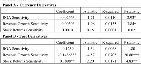
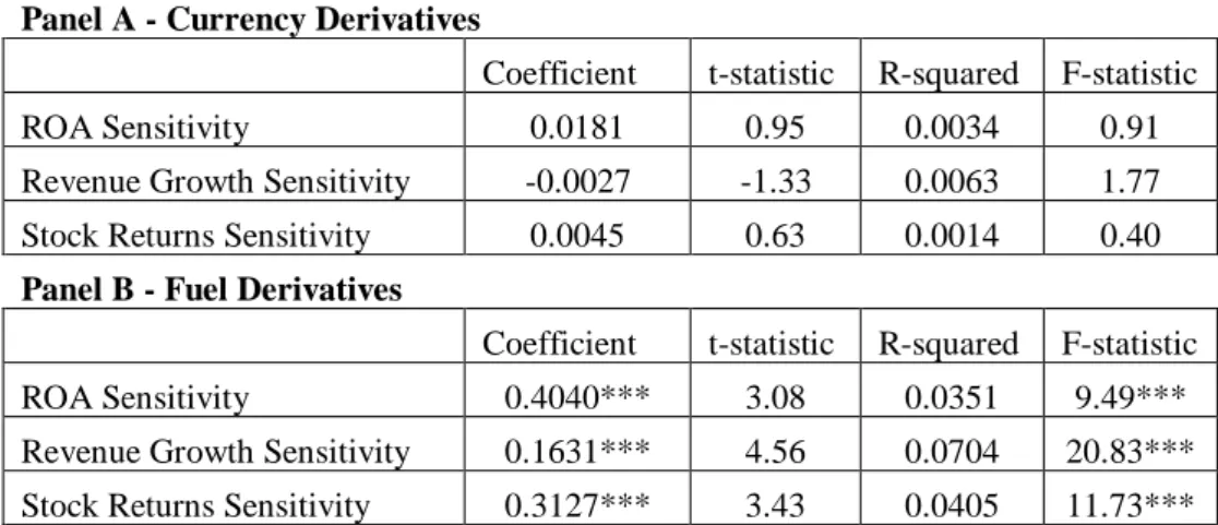
Table 8 presents the impact that the use of derivatives has on ROA, stock returns and revenue growth sensitivities, that is, the betas. We see that, for example, the use of currency derivatives decreases ROA’s sensitivity regarding currency movements (ROA’s currency beta), by 0.0266, all else equal. Broadly, we see that both the use of currency derivatives and fuel derivatives, lowers the values of the betas for ROA and revenue growth. However, the betas for stock returns increase with hedging. This means that the stock returns of a firm that uses derivatives

(25)

Table 8 – Absolute Betas

Panel A - Currency Derivatives

Coefficient t-statistic R-squared F-statistic

ROA Sensitivity -0.0266* -1.71 0.0110 2.93*

Revenue Growth Sensitivity -0.0030* -1.96 0.0135 3.84*

Stock Returns Sensitivity 0.0010 0.15 0.0001 0.02

Panel B - Fuel Derivatives

ROA Sensitivity -0.1239 -1.34 0.0068 1.80

Revenue Growth Sensitivity -0.1486*** -4.57 0.0705 20.86***

Stock Returns Sensitivity 0.1898** 2.20 0.0171 4.83**

This table presents the results of six different regressions. The dependent variables are listed in first column: ROA Sensitivity, Revenue Growth Sensitivity and Stock Returns Sensitivity. These sensitivities are the absolute values that were calculated. The independent variables are the currency derivatives dummy (panel A) and the fuel derivatives dummy (panel B). Currency derivatives dummy and Fuel derivatives dummy are variables that equal one if the firm reports using that type of derivative in its 10k annual report. ***, **, * denote significance at the 1%, 5% and 10% levels, respectively.

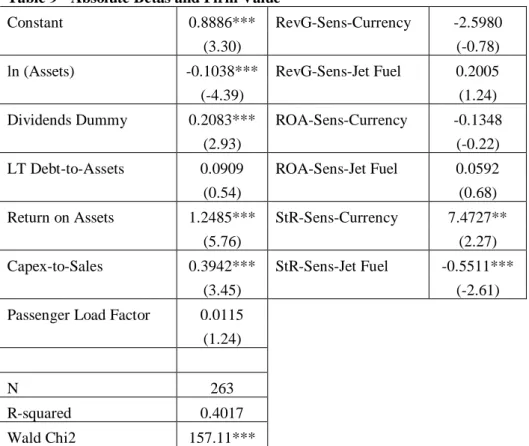
are more sensitive to changes in the price of the underlying, than if the firm was unhedged. To study how the betas influence Tobin’s Q, I am going to repeat the random effects regression of section 4.1. substituting the derivatives dummies by the betas. The results are presented in table 9.

Concerning currency betas, we see that an increase in the revenue growth beta and the ROA beta, decreases the value of Q. As we saw before, the use of foreign currency derivatives decreases these betas, which means that foreign currency hedging increases the value of Q. On the other hand, an increase in the beta for stock returns increases the value of Q. Interestingly, since we saw that the use of currency derivatives increases the beta, then this means again that currency hedging increases Q.

Regarding fuel derivatives, the results are the opposite. The coefficients for revenue growth and ROA betas are positive, while the use of fuel derivatives decreases these betas. Consequently, using fuel derivatives impacts Q negatively according to these two metrics. The coefficient on the stock returns beta is negative and since beta increases when using derivatives, then again we see that fuel hedging decreases the value of Q.

These results are consistent with the findings of 4.1. where the coefficient on fuel derivatives use had a negative sign while the coefficient on currency derivatives use had a positive sign.

(26)

Table 9 - Absolute Betas and Firm Value

Constant 0.8886*** RevG-Sens-Currency -2.5980

(3.30) (-0.78)

ln (Assets) -0.1038*** RevG-Sens-Jet Fuel 0.2005

(-4.39) (1.24)

Dividends Dummy 0.2083*** ROA-Sens-Currency -0.1348

(2.93) (-0.22)

LT Debt-to-Assets 0.0909 ROA-Sens-Jet Fuel 0.0592

(0.54) (0.68)

Return on Assets 1.2485*** StR-Sens-Currency 7.4727**

(5.76) (2.27)

Capex-to-Sales 0.3942*** StR-Sens-Jet Fuel -0.5511***

(3.45) (-2.61)

Passenger Load Factor 0.0115

(1.24)

N 263

R-squared 0.4017

Wald Chi2 157.11***

This table presents the results for a random-effects regression. The dependent variable is Tobin's Q which is the market value of assets divided by its the replacement cost of assets, following the approach of Chung and Pruitt (1994). ln (Assets) is the natural logarithm of total assets. Dividends Dummy equals one if the firm distributed dividends that year. LT Debt-to-Assets is the ratio of long-term debt to total assets. Return on Assets is the ratio of net income to assets. CAPEX-to-Sales is the ratio of capital expenditures to total sales. Passenger Load Factor is the average percentage of seats airlines are able to sell per flight. The final six regressors are the absolute betas that were calculated. RevG stands for revenue growth. ROA stands for return on assets. StR stands for stock returns. For example, ROA-Sens-Currency is the ROA currency beta. Regressions also include year dummies which are not reported. T-statistics are presented between parenthesis. ***, **, * denote significance at the 1%, 5% and 10% levels, respectively.

4.4.2. Real Betas

As stated before, we have to be much more prudent when looking into the real values of betas. A positive impact on a beta, for example, can mean that the beta became less negative, more positive, or even went from negative to positive. This means that the results in table 10, cannot be interpreted without knowing the sign of each company beta. The results in table 11, on the other hand can be interpreted, without knowing the exact sign of each beta. Note that we are now looking at how changes in betas caused by the use of derivatives, influence Tobin’s Q, whereas above we were looking into changes in sensitivity (absolute betas). Remember that in this subsection a decrease in beta, for instance, does not mean a decrease in sensitivity. In regard to currency betas, we see that only an increase in the revenue growth beta decreases the value of Q. Since the use of foreign currency derivatives decreases this beta, foreign currency hedging increases the value of Q. An increase in the betas for stock returns and ROA

(27)

Table 10 - Real Betas

Panel A - Currency Derivatives

ROA Sensitivity 0.0181 0.95 0.0034 0.91

Revenue Growth Sensitivity -0.0027 -1.33 0.0063 1.77

Stock Returns Sensitivity 0.0045 0.63 0.0014 0.40

Panel B - Fuel Derivatives

ROA Sensitivity 0.4040*** 3.08 0.0351 9.49***

Revenue Growth Sensitivity 0.1631*** 4.56 0.0704 20.83***

Stock Returns Sensitivity 0.3127*** 3.43 0.0405 11.73***

This table presents the results of six different regressions. The dependent variables are listed in first column: ROA Sensitivity, Revenue Growth Sensitivity and Stock Returns Sensitivity. These sensitivities are the real values that were calculated. The independent variables are the currency derivatives dummy (panel A) and the fuel derivatives dummy (panel B). Currency derivatives dummy and fuel derivatives dummy are variables that equal one if the firm reports using that type of derivative in its 10k annual report. ***, **, * denote significance at the 1%, 5% and 10% levels, respectively.

Table 11 - Real Betas and Firm Value

Constant 0.9661*** RevG-Sens-Currency -0.5297

(3.70) (-0.18)

ln (Assets) -0.1031*** RevG-Sens-Jet Fuel 0.3464**

(-4.71) (2.51)

Dividends Dummy 0.1920*** ROA-Sens-Currency 0.4582

(2.90) (0.82)

LT Debt-to-Assets 0.2016 ROA-Sens-Jet Fuel -0.0603

(1.16) (-0.91)

Return on Assets 1.2238*** StR-Sens-Currency 9.2678***

(5.68) (3.27)

Capex-to-Sales 0.5135** StR-Sens-Jet Fuel -0.6747***

(2.32 (-3.65)

Passenger Load Factor 0.0103***

(2.91)

N 263

R-squared 0.4178

Wald Chi2 167.90***

This table presents the results for a random-effects regression. The dependent variable is Tobin's Q which is the market value of assets divided by its the replacement cost of assets, following the approach of Chung and Pruitt (1994). ln (Assets) is the natural logarithm of total assets. Dividends Dummy equals one if the firm distributed dividends that year. LT Debt-to-Assets is the ratio of long-term debt to total assets. Return on Assets is the ratio of net income to assets. CAPEX-to-Sales is the ratio of capital expenditures to total sales. Passenger Load Factor is the average percentage of seats airlines are able to sell per flight. The final six regressors are the real betas that were calculated. RevG stands for revenue growth. ROA stands for return on assets. StR stands for stock returns. For examle, ROA-Sens-Currency is the ROA currency beta. Regressions also include year dummies which are not reported. T-statistics are presented between parenthesis. ***, **, * denote significance at the 1%, 5% and 10% levels, respectively.

(28)

increases the value of Q and using derivatives increases the values of the betas. Hedging thus increases the value of Q.

As for fuel derivatives, only the coefficient for revenue growth beta is positive, and the use of fuel derivatives increases this beta. This means that using fuel derivatives impacts Q positively, which is contrary to the previous findings. However, the coefficients on the betas for stock returns and ROA are negative and since both betas increase when using derivatives, in these cases fuel hedging decreases the value of Q.

4.5. Fifth Hypothesis

Given that the analysis has not produced results similar to previous literature, I decided to investigate the relation between fuel prices and currency prices. So far, I have analysed the use of fuel derivatives and currency derivatives, both separately and together, yielding similar outcomes. In this subsection, I will look solely into price movements of jet fuel and of the US dollar and check to see if there is a relation between the two.

As we have seen before, an increase in jet fuel costs hurts airlines’ profit margins since they cannot reflect the entire change in price on the price they charge for tickets. Concerning foreign currency, a devaluation of the US dollar, increases the value of foreign revenues. So for airlines, the ideal situation would be to have low jet fuel prices, and a cheap US dollar, whereas the contrary would be very hurtful. On the contrary, if jet fuel prices would move on the opposite direction of foreign currency, airlines would experience some sort of a natural hedge in energy and currency risks. That is, if increasing oil prices were to be correlated with decreasing dollar values, the loss on jet fuel, would be partially offset by the gain in foreign revenues and vice versa. To study this possibility, I will look into the quarterly prices from 2000 until 2016 of the two indices described in 3.3. – DXY and JETINYPR.

In figure 1 we can see the values for DXY and JETINYPR for the period mentioned. Please note that the left axis refers to the values of DXY and the right axis to JETINYPR. The correlation between the two is -0.8013, which is a strong negative correlation. This means that, during this period of our study, on average, when the cost of jet fuel went up, the US dollar depreciated, and when the cost of jet fuel decreased, the US dollar appreciated.

Airlines, as every company, face many risks that are somewhat exogenous to their activities. When choosing to control (hedge) a risk, the company is, to some extent, trying to make the variable more endogenous. If that variable happened to be correlated with another variable, by hedging it, the firm is breaking that natural correlation. The fact that, in this specific case, there

(29)

is evidence of a natural hedge, possibly indicates a reason why I do not find statistically significant evidence of a hedging premium in our sample. Investors will not value a firm’s financial decision, if they think that it is a waste of money to do so.

It is important to see that this model is extremely simple and does not look for a reasoning behind the observed correlation. Moreover, the impact of the natural hedge depends greatly on the relative impact of jet fuel costs and foreign revenues for airlines, and also on the composition of its foreign revenues. However, I believe it sets the ground for a possible future work on this particular subject and further investigation of this issue is suggested as a line for future research.

5. Conclusion

This paper studies the use of fuel and foreign currency derivatives in a sample of 26 US passenger airlines, between 2000 and 2016. The purpose was to examine how investors perceived a company that hedged fuel and currency risks, and also the reasons that may lead a company to engage in a hedging strategy.

Although the evidence found is not statistically significant, when measuring changes in Tobin’s Q relative to the use of derivatives, I see that using foreign currency derivatives causes Q to increase while using fuel derivatives decreases Q. These results are robust to several control variables such as size and investment opportunities. Looking into the likeliness of using each type of derivatives based on firm fundamentals, I find that firms are less likely to use both types

0 0.5 1 1.5 2 2.5 3 3.5 4 4.5 0 20 40 60 80 100 120 140 3/1/00 1/1/01 11/1/01 9/1/02 7/1/03 5/1/04 3/1/05 1/1/06 11/1/06 9/1/07 7/1/08 5/1/09 3/1/10 1/1/11 11/1/11 9/1/12 7/1/13 5/1/14 3/1/15 1/1/16 11/1/16 JE T IN Y P R DXY