High strain rate identification of Pinus pinaster Ait. on the transverse plane by the image-based inertial impact test

Filipa Alexandra Grifo Cunha

Graduate in Mechanical Engineering Sciences

High strain rate identification of Pinus pinaster

Ait. on the transverse plane by the image-based

inertial impact test

Dissertation submitted in partial fulfillment

of the requirements for the degree of

Master of Science in

Mechanical Engineering

Adviser:

Prof. Doutor José Manuel Cardoso Xavier,

Assistant professor,

Universidade Nova de Lisboa

Co-adviser:

Prof. Doutor Rui Fernando dos Santos Pereira Martins,

Assistant professor,

Universidade Nova de Lisboa

Examination Committee

Chair: Prof. Doutor António José Freire Mourão

High strain rate identification of Pinus pinaster Ait. on the transverse plane by the

image-based inertial impact test

Copyright c Filipa Alexandra Grifo Cunha, Faculty of Sciences and Technology, NOVA Univer-sity Lisbon.

The Faculty of Sciences and Technology and the NOVA University Lisbon have the right, perpet-ual and without geographical boundaries, to file and publish this dissertation through printed copies reproduced on paper or on digital form, or by any other means known or that may be in-vented, and to disseminate through scientific repositories and admit its copying and distribution for non-commercial, educational or research purposes, as long as credit is given to the author and editor.

This document was created using the (pdf)LA_{TEX processor, based on the “novathesis” template[1], developed at the Dep. Informática of FCT-NOVA [2].}

Acknowledgements

Em primeiro lugar, gostaria de agradecer ao meu orientador, professor José Xavier, pela sugestão do tema, pela ajuda e pelo conhecimento transmitido. E gostaria também de agradecer ao meu co-orientador, professor Rui Martins, por toda a orientação.

Quero agradecer ao professor Fabrice Pierron e a toda a equipa da Universidade de Southamp-ton pela realização dos ensaios experimentais que integram esta dissertação.

Agradeço à Faculdade de Ciências e Tecnologia da Universidade Nova de Lisboa pela for-mação e por todos os conhecimentos que adquiri neste trabalho, bem como em todo o curso.

Gostaria de agradecer aos meus colegas toda a ajuda que me deram ao longo dos 5 anos de curso.

Agradeço aos meus amigos que me acompanharam ao longo deste percurso todo o apoio e amizade. Em especial, ao meu namorado pelas palavras de carinho e motivação.

Por fim, um grande agradecimento aos meus pais e à minha irmã, por me terem apoiado, motivado e ajudado neste percurso. Obrigada por acreditarem em mim. Sem vocês nunca teria conseguido.

"Grandes batalhas só são dadas a grandes guerreiros." Mahatma Gandhi

Abstract

Computer-aided engineering systems typically rely on constitutive models and material pa-rameters to describe the mechanical behaviour of material over a spectrum of high strain rate regimes. The constitutive parameters are to be determined experimentally by suitable test meth-ods. At high strain rate regimes, a few test methods have been proposed, with advantages and drawback. More recently, an image-based inertial impact (IBII) test was proposed to overcome limitation of quasi-static stress equilibrium (neglecting inertia effects) and 1D wave propagation theory (neglecting dispersion effects) of the classical split-Hopkinson pressure bar (SHPB) test. This dynamic test rely on full-field deformation measurements provided by an optical technique and ultra high speed imaging to resolve both spatial and temporal resolutions.

Wood and wood-based products are gaining momentum due to policies of sustainability and green economy. The extension of using such materials under a higher strain rate regimes would be therefore of interest in engineering applications.

This work aims the identification of linear elastic constitutive parameters of Pinus pinaster Ait. (maritime pine) wood subjected to high strain rates, using the image-based inertial impact test. In this dynamic test, images of specimen deformation are recorded by means of an ultra high speed camera. The recorded images are processed by the grid method yielding displacement fields over the whole external surface of the specimen. Through the displacements field, the strain and acceleration fields are reconstructed, respectively, by means of spatial and temporal derivations. By using the virtual fields method (VFM), it is possible to identify the constitutive parameters of wood. This characterisation is performed without measuring external forces applied to the specimen under study by selecting VFM admissible virtual fields. This is performed using acceleration fields as a load cell, thereby taking advantage of the non-negligible inertial forces introduced during the dynamic test.

In this work, two experimental analyses are carried out on Pinus pinaster Ait. species by using specimens oriented on the RT (Radial-Tangential) and TR (Tangential-Radial) planes. Data from the experimental tests are further processed by the VFM to identify properties such as Young’s modulus (E) and Poisson’s coefficient (ν) of the material under study. In this analysis an approximation was performed, having been considered an isotropic constitutive model in the VFM, since the RT and TR planes have a low anisotropy ratio. In this study, the stiffness components (Qxx and Qxy) of the material were determined, with average values of 2.23 GPa

and 0.80 GPa, respectively, for the RT specimens. Similarly, the average values for the stiffness components (Qxx and Qxy) are 0.98 GPa and 0.80 GPa for the TR specimens. These dynamic

elastic parameters are of the same order of magnitude of quasi-static references values. Therefore, it may be concluded that high strain rate loading has a non significant influence on the elastic transverse properties of for the Pinus pinaster Ait. species. Taking into account the advent of

digital technology, the image-based inertial impact test may become a conventional test method to study the materials properties of structural engineering when subjected to high strain rate loads.

Keywords: Image-based inertial impact test, Grid method, High strain rate testing, Virtual Fields Method, Wood, Dynamic behaviour.

Resumo

Os sistemas de engenharia assistida por computador geralmente contam com modelos cons-titutivos e parâmetros do material para descrever o comportamento mecânico do material num espectro de regimes de elevadas taxas de deformação. Os parâmetros constitutivos devem ser determinados experimentalmente por métodos de ensaio adequados. Em regimes de elevadas taxas de deformação, alguns métodos de ensaio foram propostos, com vantagens e desvantagens. Mais recentemente, um ensaio de impacto inercial foi proposto para superar a limitação do equilíbrio de tensão quase-estático (efeitos de inércia negligenciados) e a teoria de propagação de ondas unidimensionais (efeitos de dispersão negligenciadas) do teste clássico de barras de pressão de split-Hopkinson. Este ensaio dinâmico baseia-se em medições dos campos de defor-mações fornecidas por uma técnica óptica e por imagens de câmaras ultra-rápidas para resolver resoluções espaciais e temporais.

A madeira e os produtos à base de madeira estão a ganhar força devido a políticas de sustentabilidade e economia verde. A extensão do uso de tais materiais sob regimes de elevadas taxas de deformação seria, portanto, de interesse em aplicações de engenharia.

Este trabalho tem como objetivo a identificação de propriedades constitutivas da madeira de espécie Pinus pinaster Ait. (pinho marítimo), sujeita a elevadas taxas de deformação, utilizando o ensaio de impacto inercial. Neste ensaio experimental foram registadas imagens da deformação do provete por meio de uma câmara ultra-rápida. As imagens captadas foram posteriormente processadas pelo método das grelhas com a finalidade de serem obtidos os campos de deslo-camentos na superfície do provete. Através do campo de deslodeslo-camentos determinaram-se os campos de deformações e de acelerações, mediante uma derivação espacial e uma derivação tem-poral de segunda ordem, respetivamente. Ao utilizar o método dos campos virtuais, é possível identificar os parâmetros constitutivos da madeira sem a medição de forças externas aplicadas no provete em estudo. Esta identificação é efetuada utilizando a aceleração como célula de carga, aproveitando deste modo as forças inerciais não desprezáveis do ensaio dinâmico.

Neste trabalho foram efetuadas duas análises experimentais com o propósito de estudar os parâmetros constitutivos de provetes da madeira de espécie de Pinus pinaster Ait. Os ensaios de impacto foram realizados em provetes com a orientação RT (Radial-Tangencial) e com orientação TR (Tangencial-Radial). Os dados provenientes dos ensaios experimentais foram posteriormente processados pelo método dos campos virtuais de forma a serem identificadas as propriedades, como o módulo de Young (E) e o coeficiente de Poisson (ν), do material em estudo. Nesta análise foi realizada uma aproximação, tendo sido considerado um modelo isotrópico e não ortotrópico no método dos campos virtuais, visto que os planos RT e TR apresentam um baixo rácio de anisotropia. Neste estudo foram determinadas as componentes da rigidez (Qxxe Qxy) do

orientados segundo o plano RT. Do mesmo modo, para os provetes orientados segundo o plano TR, os valores médios para as componentes da rigidez (Qxxe Qxy) são 0,98 GPa e 0,80 GPa.

Esses parâmetros dinâmicos elásticos são da mesma ordem de magnitude que os valores de referência quase-estáticos. Portanto, conclui-se que o carregamento a elevadas taxas de defor-mação não tem influência significativa nas propriedades transversais elásticas da madeira de Pinus pinaster Ait. Considerando o advento da tecnologia digital, o ensaio de impacto inercial pode-se tornar um método de ensaio convencional para estudar as propriedades dos materiais da engenharia estrutural quando submetidos a elevadas taxas de deformação.

Palavras-chave: Ensaio de impacto inercial, Método das grelhas, Elevadas taxas de deformação, Método dos Campos Virtuais, Madeira, Comportamento dinâmico.

Contents

1 Introduction 1

1.1 Background . . . 1

1.2 Objectives . . . 2

1.3 Structure . . . 2

2 Dynamic impact behaviour of materials 5 2.1 Introduction . . . 5

2.2 Material behaviour at high strain rates. . . 5

2.2.1 Numerical modelling . . . 5

2.2.2 Experimental techniques . . . 7

2.3 Conclusion . . . 15

3 Wood structure and behaviour 17 3.1 Introduction . . . 17

3.2 Softwood and hardwood species . . . 18

3.3 Wood of softwood species . . . 19

3.3.1 Macroscopic structure . . . 19

3.3.2 Microscopic structure . . . 20

3.3.3 Variability in structure . . . 21

3.3.4 Directions of wood material symmetry . . . 22

3.4 Wood characterization at high strain rates. . . 23

3.4.1 Intermediate strain rate testing . . . 23

3.4.2 Transverse impact . . . 24

3.4.3 Longitudinal impact: high strain rate . . . 25

3.5 Conclusion . . . 26

4 Methodologies 27 4.1 Introduction . . . 27

4.2 Image-based inertial impact test . . . 28

4.3 Grid Method . . . 29

4.3.1 Ultra high speed imaging . . . 33

4.4 Virtual Fields Method . . . 37

4.4.1 Virtual Works Principle . . . 37

4.4.2 Constitutive equation of elastic linear behaviour. . . 39

4.4.3 Virtual Fields Method Using Inertial Forces . . . 43

C O N T E N T S

5 Experimental analysis 49

5.1 Introduction . . . 49

5.2 Experimental procedure . . . 49

5.3 RT oriented specimen . . . 50

5.3.1 Results and discussion . . . 51

5.4 TR oriented specimen . . . 62

5.4.1 Results and discussion . . . 62

5.5 Conclusion . . . 73

List of Figures

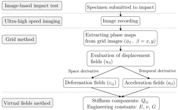
1.1 Flow chart of procedures and methodologies of this thesis.. . . 3

2.1 Experimental techniques as function of strain rate (Ramesh, 2008). . . 8

2.2 Test duration and strain rates for different tests (Longana, 2014). . . 8

2.3 Instron VHS machine schematic (Longana, 2014). . . 9

2.4 Schematic of the normal plate impact test (Yuan et al., 2007). . . 9

2.5 Schematic representation of the experimental technique of Split-Hopkinson pressure bar (Ramesh, 2008). . . 10

2.6 Lagrange diagrams: (a) just after the impact on the striker/incident bars; (b) through time and space in the experimental technique of split-Hopkinson pressure bar (Ramesh, 2008). . . 12

2.7 Signals usually recorded on strain gauges on the input bar and output bar (Ramesh, 2008). . . 13

3.1 Anatomic structure: a) softwood specie; b) hardwood specie [adapted from (Xavier, 2003)].. . . 18

3.2 Hardwood species classification: (a) ring porosity; (b) diffuse porosity (Xavier, 2003). 19 3.3 Macroscopic structure of the trunk of a softwood specie (Dinwoodie, 2000). . . 20

3.4 Microscopic aspects of the wood of softwood species (Garrido, 2004). . . 21

3.5 Representation of the cell wall structure (Dinwoodie, 2000). . . 22

3.6 Orthonormal material symmetry direction of wood within the stem (Xavier, 2003). . 23

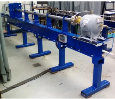
4.1 Inertial impact test (from PhotoDyn project). . . 28

4.2 Representative scheme of the physical components of inertial impact test (Fletcher and Pierron, 2018). . . 29

4.3 Representative scheme of inertial impact test sample when loaded with a compression pulse (Fletcher and Pierron, 2018). . . 29

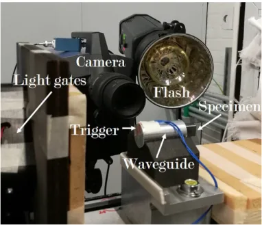
4.4 (a) Photograph of experimental ultra high speed camera, light flash and sample. (b) Projectile and its base. (c) Test specimen of the wave and foam support (Fletcher and Pierron, 2018). . . 30

4.5 Illustrative image of: (a) cross grid, I(x, y); (b) grid with vertical lines, Ix(x, y) (propor-cional a ux(x1, x2)); (c) grid with horizontal lines, Iy(x, y)(proportional to uy(x1, x2)) (Xavier, 2007). . . 30

4.6 Example of a grid (from PhotoDyn project). . . 31

4.7 Displacement of a physical point (Grédiac et al., 2016). . . 32

4.8 High speed and ultra high speed cameras available on the market [adapted from (Reu and Miller, 2008)].. . . 34

L i s t o f F i g u r e s

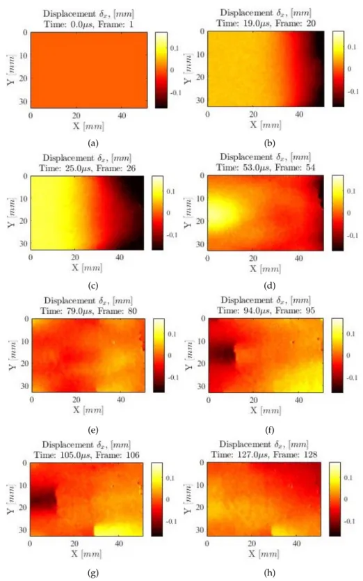
4.10 Solid shape subject to mechanical load (Pierron and Grédiac, 2012). . . 38 4.11 Global and fibre coordinate system. . . 40 4.12 Schematic representation of a dynamic uniaxial test, adapted from (Pierron et al., 2014). 41 5.1 Schematic representation of the simulated test. . . 50 5.2 Maps of the x components of the displacements for a specimen with RT orientation

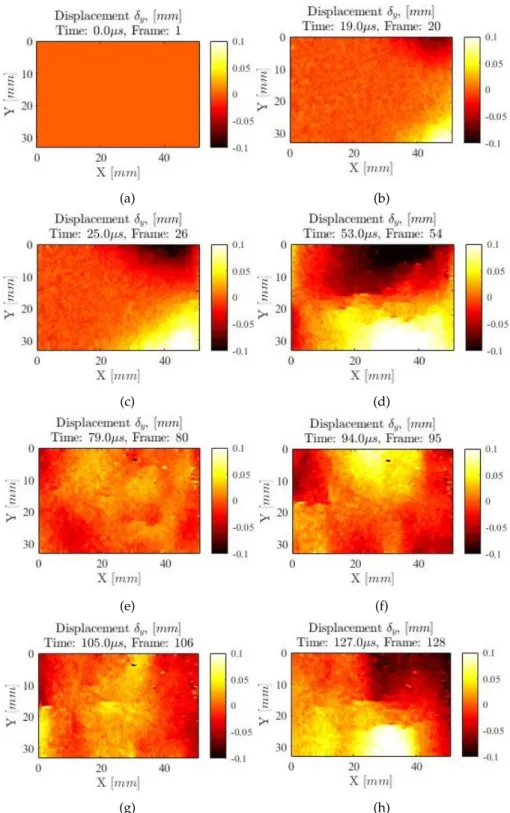
at various times. (a) t=0µs. (b) t=19µs. (c) t=25µs. (d) t=53µs. (e) t=79µs. (f) t=94µs. (g) t=105µs. (h) t=127µs. . . . 52 5.3 Maps of the y components of the displacements for a specimen with RT orientation

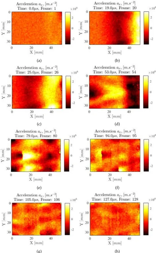
at various times. (a) t=0µs. (b) t=19µs. (c) t=25µs. (d) t=53µs. (e) t=79µs. (f) t=94µs. (g) t=105µs. (h) t=127µs. . . . 53 5.4 Maps of the x components of the accelerations for a specimen with RT orientation at

various times. (a) t=0µs. (b) t=19µs. (c) t=25µs. (d) t=53µs. (e) t =79µs. (f) t=94µs. (g) t=105µs. (h) t=127µs. . . . 54 5.5 Maps of the y components of the accelerations for a specimen with RT orientation at

various times. (a) t=0µs. (b) t=19µs. (c) t=25µs. (d) t=53µs. (e) t =79µs. (f) t=94µs. (g) t=105µs. (h) t=127µs. . . . 55 5.6 Maps of the x components of the strains for a specimen with RT orientation at various

times. (a) t=0µs. (b) t=19µs. (c) t=25µs. (d) t=53µs. (e) t=79µs. (f) t=94µs. (g) t=105µs. (h) t=127µs. . . . 56 5.7 Maps of the xy components of the strains for a specimen with RT orientation at various

times. ((a) t=0µs. (b) t=19µs. (c) t=25µs. (d) t=53µs. (e) t=79µs. (f) t=94µs. (g) t=105µs. (h) t=127µs. . . . 57 5.8 Maps of the y components of the strains for a specimen with RT orientation at various

times. (a) t=0µs. (b) t=19µs. (c) t=25µs. (d) t=53µs. (e) t=79µs. (f) t=94µs. (g) t=105µs. (h) t=127µs. . . . 58 5.9 Maps of the comparison of strain on RT orientation specimen before and after

smooth-ing at time t=180µs.. . . 59 5.10 Results obtained for stiffness component Qxxover time t on RT orientation specimen. 60

5.11 Results obtained for stiffness component Qxyover time t on RT orientation specimen. 60

5.12 Results obtained for the Young’s modulus along x position on RT orientation specimen. 61 5.13 Results obtained for the Young’s modulus over time t on RT orientation specimen. . 62 5.14 Maps of the x components of the displacements for a specimen with TR orientation

at various times. (a) t=0µs. (b) t=20µs. (c) t=26µs. (d) t=39µs. (e) t=47µs. (f) t=50µs. (g) t=57, 5µs. (h) t=63, 5µs. . . . 63 5.15 Maps of the y components of the displacements for a specimen with TR orientation

at various times. (a) t=0µs. (b) t=20µs. (c) t=26µs. (d) t=39µs. (e) t=47µs. (f) t=50µs. (g) t=57, 5µs. (h) t=63, 5µs. . . . 64 5.16 Maps of the x components of the accelerations for a specimen with TR orientation at

various times. (a) t=0µs. (b) t=20µs. (c) t=26µs. (d) t=39µs. (e) t =47µs. (f) t=50µs. (g) t=57, 5µs. (h) t=63, 5µs. . . . 65 5.17 Maps of the y components of the accelerations for a specimen with TR orientation at

various times. (a) t=0µs. (b) t=20µs. (c) t=26µs. (d) t=39µs. (e) t =47µs. (f) t=50µs. (g) t=57, 5µs. (h) t=63, 5µs. . . . 66

L i s t o f F i g u r e s

5.18 Maps of the x components of the strains for a specimen with TR orientation at various times. (a) t=0µs. (b) t=20µs. (c) t=26µs. (d) t=39µs. (e) t=47µs. (f) t=50µs. (g) t=57, 5µs. (h) t=63, 5µs. . . . 67 5.19 Maps of the xy components of the strains for a specimen with TR orientation at

various times. (a) t=0µs. (b) t=20µs. (c) t=26µs. (d) t=39µs. (e) t =47µs. (f) t=50µs. (g) t=57, 5µs. (h) t=63, 5µs. . . . 68 5.20 Maps of the y components of the strains for a specimen with TR orientation at various

times. (a) t=0µs. (b) t=20µs. (c) t=26µs. (d) t=39µs. (e) t=47µs. (f) t=50µs. (g) t=57, 5µs. (h) t=63, 5µs. . . . 69 5.21 Comparison of deformation cartographies on an TR orientation specimen before and

after smoothing at time t=180µs. . . . 70 5.22 Results obtained for stiffness component Qxxover time t on TR orientation specimen. 70

5.23 Results obtained for stiffness component Qxyover time t on TR orientation specimen. 71

5.24 Results obtained for the Young’s modulus along x position on TR orientation specimen. 72 5.25 Results obtained for the Young’s modulus over time t on TR orientation specimen. . 72

List of Tables

4.1 Shimadzu HPVX camera specifications. . . 36 5.1 Properties of constituent components of the image-based inertial impact test (Xavier,

2003). . . 50 5.2 Results obtained for the constitutive parameters of Pinus pinaster Ait. wood for

differ-ent specimens with oridiffer-entation in the RT plane. . . 61 5.3 Results obtained for the constitutive parameters of Pinus pinaster Ait. wood for

1

Introduction

1.1

Background

Materials used for structural engineering purposes are subjected to different deformation rates. When subjected to impact, collision or explosion, they are exposed to high strain rates. Therefore, it is important to characterize materials subject to high strain rates as they have a variety of applications, namely in the aeronautical industry, marine shipping, as well as in construction, manufacturing processes and military applications. However, characterizing the behaviour of materials and identifying their properties at high strain rates demonstrate several experimen-tal difficulties. To obtain the constitutive parameters of a material it is necessary to perform experimental tests (Meyers,2007).

Experimental test methods are carried out at specific strain rates, which refers to the maximum strain value achieved during the test (Ramesh, 2008). Some of the experimental tests used to characterize materials at various strain rates are servo hydraulic testing machine, pressure-shear plate impact and Split-Hopkinson pressure bar.

The quasi-static behaviour of materials has been extensively studied to determine parameters governing the constitutive models for this regime of strain rate. However, data at the high strain rate regimes is more scarce and less consensual. The dynamic behaviour involves inertia effects and load measurements which are more difficult to measure experimentally.

A few test methods have been proposed to address the dynamic mechanical behaviour of materials. Among them the gold standard is the SHPB. In this experimental test load cells are used to measure the force applied to the specimen and the associated strain rates (Zhu, 2015). This experimental test has some limitations that need to be addressed in order to have a more accurate characterization of materials.

Since many years ago, wood has been used by man as a building material. Today there are several utilities in engineering where this biological material is applied (Gibson and Ashby, 1999). Wood is a material that presents unusual characteristics such as anisotropy, variability and great heterogeneity (Kollmann and Côté,1968). In order to use wood as a structural material, it is important to understand the constitutive properties of this material in its three orthonormal material planes (longitudinal, radial and tangential). Due to its characteristics of anisotropy and variability, conducting experimental tests on wood becomes an arduous task. When it comes to experimental tests at high strain rates, the difficulty of studying this material increases.

In recent years there has been an increase in studies using optical techniques to perform displacement and strain field measurements. This increase is due to the improved computing power and ultra high speed cameras available on the market. Digital image correlation and

C H A P T E R 1 . I N T R O D U C T I O N

the grid method are some of the existing optical techniques in the scientific community (Pier-ron and Forquin,2012). In the 80s, optical techniques began to be used in more complex test configurations, as image processing made it possible to process experimental data more automat-ically. Prior to optical techniques, the processing of data obtained in experimental tests was done manually. These techniques could only provide quantitative measurements of stress and strain distributions from a limited number of points because of prolonged data collection procedures. Thus, these techniques were only used in specialized laboratories (Pierron and Grédiac,2012). Such techniques have been piquing the interest of the scientific community of experimental mechanics as their potential is seen as revolutionary of experimental material testing. Optical techniques allow the fields of heterogeneous deformation to be obtained in a specimen, and after this analysis it is possible to obtain the constituent parameters of the material in a dynamic test. Identification of the constituent properties of a material is achievable without measuring exter-nal forces applied to the specimen, however this type of process requires inverse techniques. The principle of virtual work was started to be used as a tool to identify the constitutive parameters of materials. Based on this, the virtual field method was used to identify material properties using acceleration as a load cell, thus taking advantage of inertial effects (Pierron et al., 2014). The virtual field method when compared to other inverse methods, such as the finite element model updating method, has a higher computational efficiency, as this technique does not require iterative resolutions (Pierron and Forquin,2012).

In recent years, an effort has been made to study the effects of strain rates on metal properties, but studies of wood properties have been increasing as it has appeared as a structural material, replacing metal (Polocoser et al.,2017).

1.2

Objectives

The aim of this thesis is to identify the constitutive parameters of Pinus pinaster Ait. wood at high strain rates through the image-based inertial impact test. In this experimental and dynamic test, images of specimen deformation will be recorded through an ultra high speed camera. These images will be further processed by the grid method in order to obtain the displacement fields on the specimen surface. Subsequently, the strains and accelerations fields will be determined from the displacements fields, by means of a spatial derivation and a second order temporal derivation, respectively. The virtual fields method will allow to identify the constitutive parameters of the wood without measuring external forces applied to the specimen, using acceleration as a load cell. This will take advantage of the non-negligible inertial forces that exist in the dynamic test. The experimental results of the constitutive parameters will be compared with the reference values and later conclusions will be made about them. Figure1.1represents a flowchart of all the procedures and methodologies studied ih this thesis.

1.3

Structure

This thesis is divided into five chapters which are described below. In chapter 2 the theme of dy-namic behaviour of materials will be presented. In this chapter will be describe some applications where materials are subjected to high strain rates when they are subjected to impact, collision or explosion. Next, some computer aided engineering systems and their application in some activities will be reported. The finite element method will be detailed as one of the most relevant

1 . 3 . S T R U C T U R E

Figure 1.1: Flow chart of procedures and methodologies of this thesis.

CAE techniques. The experimental techniques and associated methodologies to characterize the materials in engineering will be characterized later. First, the servo hydraulic testing machine will be described, then the pressure-shear plate impact and then the split-hopkinson pressure bar. Moreover, emphasis will be given to the data reduction of the classical SPHB based on 1D ware propagation theory and strain gauge measurements to extract the stress-strain behaviour of the materials.

The chapter 3 will present the behaviour and structure of wood. The two types of wood species classifications will be compared to their internal structure: softwood and hardwood. More emphasis will be given to the softwood species as the wood under study, Pinus pinaster Ait., is classified as a softwood species. Since Pinus pinaster Ait. wood was selected for this study, more emphasis will be given to the softwood species. The macroscopic and microscopic structure of the softwood species will be described, as well as the orthogonal directions and the respective orthogonal planes. Finally, the literature on the dynamic behaviour of wood at intermediate strain rate testing, transverse impact and longitudinal impact at high strain rates will be reviewed.

The chapter 4 will expose the methodologies studied and used in this work. Initially, the image-based inertial impact test will be described as an alternative test to SHPB, in order to determine the dynamic behaviour of materials when subjected to high strain rates. Next, the optical grid method will be presented, in which the principle and grid transfer techniques are emphasized. Next, an optical technique, the grid method, will be presented which will detail the process of elaborating the grid pattern. Ultra high speed cameras will be referred to in this chapter as the sensors used to capture images in the IBII test. Next, will be characterized the ultra high speed camera used in the dynamic test under study. To end with, the VFM will be presented as an inverse method for the extraction of dynamic elastic properties from full-field deformation measurements. The principle of virtual works will be stated as the principle which the method of

C H A P T E R 1 . I N T R O D U C T I O N

virtual fields is based. The constitutive equation for materials with a linear elastic behaviour will be demonstrated. It will be explained how it is possible to use acceleration as a load cell without having to measure applied external loads. Finally, the virtual field method will be developed using the inertial forces, in order to demonstrate the identification of the constituent parameters for an isotropic material and an ortotropic material.

The chapter 5 describes the experimental analysis of the image-based inertial impact test. Two experimental tests will be made in which the specimen has different orientations, RT plane orientation and TR plane orientation. For both experimental tests, the maps of the displacement x and y components, the acceleration x and y components, and the strain x, xy and y components will be presented. The results obtained for the constitutive parameters of the Pinus pinaster ait. wood for the different specimens analysed will be exposed and compared with the reference values. Finally, the results obtained for both experimental analyses and conclusions will be discussed.

2

Dynamic impact behaviour of

materials

2.1

Introduction

In this chapter, a review on the dynamic impact behaviour of engineering materials is presented. Both numerical and experimental approaches are considered. In particular, the experimental techniques typically used for studying the impact behaviour of materials are summarised, em-phasising their application, assumptions and current limitations. Firstly, the materials behaviour at high strain rates is mentioned, emphasizing CAE systems and numerical simulation. Fol-lowing, some experimental techniques are specified, such as servo hydraulic testing machine, pressure-shear plate impact and split-hopkinson pressure bar.

2.2

Material behaviour at high strain rates

In various engineering fields, materials can be submitted to high strain rate deformations when subject, for instance, to impact, collision or explosion. Some industrial applications are listed as follows:

(i) Infrastructures and transports: Infrastructures such as power stations, large buildings, dams, bridges, must be designed to withstand natural disasters or explosions; transports must be design to sustain a certain level of dynamic impact.

(ii) Manufacturing processes: knowledge of the mechanical behaviour of materials when sub-jected to high deformation rates is essential to improve manufacturing processes in order to reduce costs and improve quality.

(iii) Civil and military applications: for the design of infrastructures and vehicles subjected to impact, as in an effective shielding project it becomes necessary to know the behavior of the materials at high deformation rates.

Therefore, it is fundamental to address the behaviour of materials at high rate strain regimes, both computationally and experimentally.

2.2.1

Numerical modelling

Computer Aided Engineering (CAE) deals with the use of computer programs to improve prod-uct design as well as to solve engineering problems in a wide range of industries (SIEMENS,

C H A P T E R 2 . D Y N A M I C I M PA C T B E H AV I O U R O F M AT E R I A L S

2018). CAE systems had been introduced in early stages of computers since 1950. In 1960, com-panies introduced a system that used the computer to monitor a large number of logic diagrams before the emergence of integrated circuits. At that stage, the term Design Automation or Auto-mated Design was coined. In the same decade, interactive graphics were then developed, giving rise to the designation of Computer Aided Design (CAD) systems. With progressive computer hardware improvements and theoretical consolidation of numerical algorithms, the second and third generation of CAE systems were developed. However, the effective utilization of such computer-based systems into the industry was relatively slow, considering the high prices of computer components at the time. It was not until the end of 1960 that CAE systems grew, due to the decline in computer hardware costs and the advent of minicomputer (Green, 1983). In engineering, generically, the CAE systems are applied in several activities, namely:

(i) Structural, thermal, kinematic, dynamic analysis, vibrations and electromagnetic, using the Finite Element Analysis (FEM).

(ii) Acoustic analysis using the FEM or the Boundary Element Method. (iii) Analysis of control systems.

(iv) Fluid and thermodynamics analysis using Computational Fluid Dynamics (CFD). (v) Analysis of mechatronic systems.

(vi) Simulation of manufacturing processes.

CAE systems have several advantages, namely the reduction of cost and time for manufac-turing and product development. Research and technological development activities are able to perform numerical simulations with CAE systems, reducing the number of prototypes and experimental tests, mitigating costs and time (SIEMENS,2018).

The FEM is one of the fundamental techniques of CAE. This method consists, in brief, of mod-elling and analysing a problem of a continuous medium through several discrete elements. The governing partial differential equations (equilibrium equations, strain-displacement relationships, compatibility equations, constitutive law) can then be solved for a finite number of kinematic or primary variables. It is necessary to specify the component geometry, the constitutive model of the materials and the boundary conditions of the problem (i.e. either prescribed displacements or applied tractions). The development of the FEM occurred in parallel to the evolution of CAE systems. The method was eventually established in the 1940’s, when Richard Courant had proposed a discretization methodology for continuous elements. In the following decade, the triangle element was introduced, capable to analyse complex geometries with suitable accuracy if numerical convergence could be achieved. The term ”Finite Element“ arose in 1960, by Ray Clough. In the 1980s, geometry standards were developed through FEA and CAD; thus, the use of 2D drawing has progressed to the use of 3D modelling. Soon after the simulation appeared in 3D; the FEA was introduced in product designs. In the year 1990, the computer and these technologies became accessible in large scale to professional users.

The finite element method can be applied to the analysis and study of many diverse engineer-ing phenomena and problems such as studyengineer-ing vibratory systems, analysengineer-ing material behaviour, solving heat conduction problems and fluid mechanics, electricity and magnetism, impact, plastic

2 . 2 . M AT E R I A L B E H AV I O U R AT H I G H S T R A I N R AT E S

conformation of materials, metallic and non-metallic structures, dimensioning of large structures, hydrodynamics, aerodynamics, among others.

In the modelling of the behaviour of materials, the finite element method allows taking into account a wide variety of constitutive models, namely, linear elasticity (Hooke’s law), plasticity, viscoplasticity, hyperplasticity, thermoelasticity, among others.

The finite element method, through numerical simulation, can identify and predict any design problems. When the material behaviour involves high strain rates, it implies the use of explicit algorithms in the finite element method, which is considered a non-linear analysis. Non-linear phenomena can exhibit three distinct types of behaviour, static, quasi-static or dynamic. The behaviour is said to be static when the load does not vary over time or when the load application time is gradual enough that the accelerations are small. A problem is called quasi-static when the inertial effect is negligible and its response varies over time as it does in static behaviour. Dynamic behaviour is characterized by having significant loading frequencies and inertial forces are not negligible. There are two types of problems of dynamic phenomena: wave propagation and structural dynamics. The wave propagation problem is associated with impact or collision phenomena, ie high frequency temporal phenomena and short analysis periods. The problem of structural dynamics is associated with situations of excitation frequencies of the order of the first natural frequency of the system (Teixeira-Dias et al.,2018).

The effective numerical simulation or prediction of CAE/FEM systems strongly rely on the constitutive models of the materials as well as their input mechanical parameters. These models must be able to simulate the material or structures behaviour for different loading scenarios. The mechanical properties of material are to be determined experimentally through suitable mechanical tests or techniques over a spectrum of strain rate regimes.

2.2.2

Experimental techniques

With the advent of computational mechanics, it is possible to perform increasingly precise numer-ical simulations of complex problems in engineering. However, it is necessary to validate these models, namely with respect to the constitutive laws and their material parameters. There are several techniques and methodologies associated with experimental mechanics for the character-ization of engineering materials (Carlsson et al.,2014). They can be classified as a function of the strain rate at which load is applied, as shown in Figure2.1(Ramesh,2008). The universal and servo-hydraulic test machines allow to perform quasi-static mechanical tests and moderate strain rate tests up, to the order of 200 s−1. Above 102 s−1, the inertial effects and acceleration must be taken into account in the material characterisation (Zhu and Pierron,2016). In the following, the most relevant high strain rate techniques are reviewed with special emphasis to the classical split-Hopkinson pressure bar (SHPB) test and analysis (Chen and Song,2011).

2.2.2.1 Servo hydraulic testing machine

In recent years servo hydraulic testing machine has become more common, as it has a range of approximately six orders of magnitude of strain rates (10−3to 10+3s−1), as shown in figure2.2 (Bardenheier and Rogers,2006).

Servo hydraulic testing machine are used for various types of impact loads such as dynamic stresses, compression, bending or shear loads (Bardenheier and Rogers, 2006). Figure2.3is a diagram of the Instron VHS 1000 machine consisting of a typical servo hydraulic testing machine.

C H A P T E R 2 . D Y N A M I C I M PA C T B E H AV I O U R O F M AT E R I A L S

Figure 2.1: Experimental techniques as function of strain rate (Ramesh,2008).

Figure 2.2: Test duration and strain rates for different tests (Longana,2014).

This machine operates by accumulating oil at a pressure of 280 bars in a pressure cylinder controlled by a proportional valve. One of the advantages of servo hydraulic machines is that they can test materials from quasi-static to intermediate strain rates (Zhu,2015).

Servo hydraulic testing machine allow the use of samples with dimensions similar to those used in quasi-static tests, thus allowing a suitable surface for full-field strain measurement techniques. With the development of ultra high speed cameras, it is possible to capture images with high temporal resolution during tests of intermediate strain rates, such as servo hydraulic testing machine.

2.2.2.2 Pressure-shear plate impact

The pressure-shear plate impact technique was developed to study the shear behaviour of ma-terials subjected to high strain rates (105to 107s−1). This test consists of the impact of two flat and parallel plates, as shown if figure 2.4. The specimen needs to be thin and flat, which is glued to the flyer. This plate is launched from a barrel of a gas gun towards the fixed plate. The plates may have different angles of incidence (Ramesh,2008). The analysis of this test consists of measuring the velocity of free particles on the surface opposite the impact (Yuan et al.,2007).

2 . 2 . M AT E R I A L B E H AV I O U R AT H I G H S T R A I N R AT E S

Figure 2.3: Instron VHS machine schematic (Longana,2014).

Figure 2.4: Schematic of the normal plate impact test (Yuan et al.,2007).

2.2.2.3 Split-Hopkinson pressure bar (SHPB)

The SHPB, or as it is also so called, the Kolsky bar, is the classical experimental test for material characterisation at high strain rate deformation (Chen and Song, 2011; Ramesh, 2008). The test was first developed in 1914 by Bertram Hopkinson to measure the elastic (stress) wave propagation in a metal bar. Later on, in 1949, Herbert Kolsky refined the original set-up by using two Hopkinson bars in series along with the sample, providing stress and strain measurements during the dynamic test. No recently, modifications were introduced allowing other loading configurations, in both tension and shear (Sudheera et al., 2018). The term SHPB is generally used when dealing with materials subjected to compression, whilst the term Kolsky bar can

C H A P T E R 2 . D Y N A M I C I M PA C T B E H AV I O U R O F M AT E R I A L S

Figure 2.5: Schematic representation of the experimental technique of Split-Hopkinson pressure bar (Ramesh,2008).

be more broadly used for compression, traction, shear or a combination among them (Ramesh, 2008).

In general, the SHPB test method is designed to achieve a uniform and uniaxial state of stress and strain on the specimen, so a direct or explicit identification can be proposed in the data reduction. The typical set-up is shown in Figure2.5. This mechanical system consists of three slender cylindrical bars axially aligned with each other. The specimen of the material under analysis is sandwiched in between the so called incident (input) and transmitted (output) bars. The smallest bar, so called striker bar, is fired at the incidence bar at an initial velocity v0, through

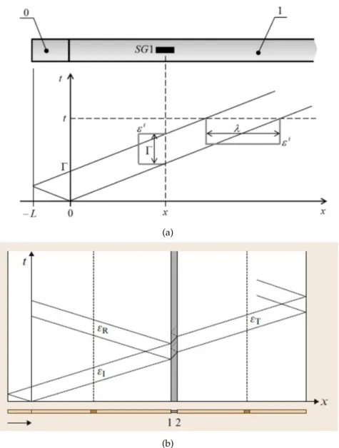
a compressed gas gun (consisting of a reservoir of pressurized stored gas). This impact generates a stress wave that propagates along the bars deforming the specimen at a high strain rate. In general, the (striker, incident and transmitted) bars have the same diameter and are made of the same material (i.e. aluminium, steel, titanium). It is assumed that their mechanical behave is confined to the linear elastic domain during the impacted test, so no permanent deformation occurs (Ramesh,2008). The lateral cross-section of the bars together with the specimen loading faces must have flatness and parallelism geometric tolerances and roughness approximating the perfect contact between both striker/incident bars and at the interfaces incident bar/specimen and specimen/transmitted bar. The bars are supported by bearings (to minimize friction effects) and must have coincident axes to ensure that wave propagation is one-dimensional (Chen and Song, 2011). Generally, the material of the bars has a higher stiffness and yield strength with regard to the specimen to be tested (Ramesh, 2008). The analysis of the test assumes that the specimen remain in contact with both the incident and transmitted bars during the period of the dynamic test, guaranteeing the continuity of the displacement field and axial stresses at the interfaces (Fletcher and Pierron,2018).

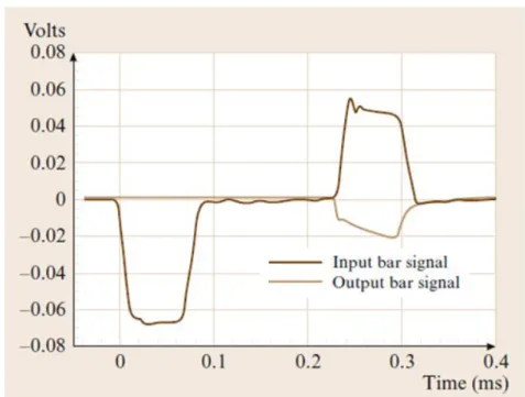
The measurement system of the SHPB test consists essentially of two subsystems (Figure2.5), one for measuring the velocity of the striker bar and another to measure the wave deformation travelling along the bars during the test. The strain signals over time are measured using one-element strain gauges glued at the surface of the incidence and transmission bars at given distance with regard to the interfaces incident bar/specimen and specimen/transmitted bar, so pulses (strain) signals can be perfectly distinguishable with no overlapping effects (Chen and Song, 2011; Meyers, 2007; Ramesh, 2008). Therefore, three pulses are typically recorded: the pulse generated by the projectile over the incident bar; the pulse reflected at the interface incident bar/specimen; and the pulse that is transmitted through the interface specimen/transmitted bar

2 . 2 . M AT E R I A L B E H AV I O U R AT H I G H S T R A I N R AT E S

(Ramesh,2008). The strain gauge signals are properly amplified and conditioned before being stored in a computer for further data reduction.

On the analysis of the input pulse, created by the impact of the striker and incident bars at a given velocity v0, it can conclude that two compressive waves are actually generated and

propagate at constant speed c (where, c= (E/µ)−1with E the Young’s modulus and µ the bar density) as can be seen by the characteristic lines on the Lagrange diagram of figure2.6a (Chen and Song, 2011; Meyers, 2007; Ramesh, 2008). On the one hand, a wave is generated which propagates in the incidence bar towards the x axis and, on the other hand, a wave is reflected and propagates in the impact bar in the negative direction of x. This latter wave reaches the free edge of the striker bar and suffers total reflection back in the positive direction of x as a tension wave at the end of the time given by (Figure2.6a):

Γ= 2L

c (2.1)

where L is the length of the striker bar and c is a constant determined as a function of the density and Young’s modulus of the bar material. This wave is continuing propagating in the incident bar, determining both the total duration (Γ) and extension (λ) of the input impulse measured by the strain gauge in the bar (Figure2.6a):

λ=2L (2.2)

The amplitude of the wave generated on the incidence bar (incident wave) can be determined by applying the linear momentum conservation equation to the system consisting of the striker and incidence bars (Meyers,2007):

µALv0=µAλv (2.3)

in which A is the cross-section area of the bars and v is the velocity at positions: ct<x <ct+λ, when t>Γ. By replacing equation (2.2) into equation (2.4) it is conclude that:

v= v0

2 (2.4)

Considering D’Alembert solution of the 1D wave equation (second-order linear partial dif-ferential equation representing the linear momentum equilibrium of the mechanical system) the strain and velocity fields are related by (Meyers,2007):

ε(x, t) = −1

cv(x, t) (2.5)

where v(x, t)represent the position of a particle at position x in the instant t. Therefore, the strain-time signal recorded by the strain gauge mounted on the incident bar (ε_SG1I ) can be obtained by replacing Eq. (2.4) in Eq. (2.6):

εI_SG1= −v0

2c (2.6)

In the Lagrange wave propagation diagram for th SHPB set-up is schematically shown in figure2.6b, neglecting the specimen dimensions (Chen and Song,2011; Meyers,2007; Ramesh, 2008). The strain-time signals are represented over time, where the incident strain is denoted by εI, the reflected strain by εR, and the transmitted strain is denoted by εT. The input stress wave

C H A P T E R 2 . D Y N A M I C I M PA C T B E H AV I O U R O F M AT E R I A L S

(a)

(b)

Figure 2.6: Lagrange diagrams: (a) just after the impact on the striker/incident bars; (b) through time and space in the experimental technique of split-Hopkinson pressure bar (Ramesh,2008).

propagates through the incident bar until reaching the specimen. At the incident bar/specimen, the wave is split; one part is reflected (as a tensile wave propagating in the negative direction of x), since the impedance (geometry and properties) of the specimen (Zp) is lower than the impedance

of the incident bar (ZI), i.e. Zp<ZI, and another part is transmitted through the specimen. The

partially reflected wave is recorded by the strain gauge at the incident bar as a tensile pulse. The transmitted wave, on the other hand, reaches the interface specimen/transmitted bar. Here the wave suffers a similar dispersion behaviour. The assumption of quasi-static stress equilibrium assumes that the stress wave reverberates multiple times at the specimen interfaces with the bars until acceleration is damped out, loading the specimen in compression at high strain rates. Therefore, inertial effects can be neglected in the data reduction. The wave is transferred to the transmitted bar as a compression impulse sine Zp<ZT (where ZTrepresents the impedance of

the transmitted bar). This impulse is recorded by the strain gauge bounded on the transmitted bar. Figure2.7shows an example of the strain signals usually recorded on the input and output

2 . 2 . M AT E R I A L B E H AV I O U R AT H I G H S T R A I N R AT E S

Figure 2.7: Signals usually recorded on strain gauges on the input bar and output bar (Ramesh, 2008).

bars strain gauges.

The analysis of the SHPB assumes that the compressive impulse generated by the striker bar is one-dimensional along the longitudinal axis. The 1D wave propagation theory is therefore proposed as data reduction. In other words, no dispersion of the pulse signal is accounted for. This assumption is never fully achievable in practice and the pulse signals can present therefore osculations (dispersion effects). In order to mitigate this issue, pulse shaping techniques have been proposed (Koerber et al.,2010). On the other hand, the size of the specimen is very short with regard to the length of the bars to ensure the condition of quasi-static equilibrium (Meyers, 2007).

The time impulse signals measured during the impacted test by the two linear strain-gauges, fixed to the incident and transmitted bars, are the basic experimental data measured for the SHPB analysis. The dynamic stress–strain response of the specimen can then be evaluated from these measurements (the incident, the reflected, and the transmitted strain-time pulses). Let’s start by analysing the velocity of a particle at the interface incident bar/specimen (x=0) given by the contribution of both incident and reflected waves:

v(0, t) ≡v1(t) =vI(0, t) +vR(0, t) =c[εR(t) −εI(t)] (2.7)

In turn, the velocity of a particle at the interface specimen / transmitted bar (x=Ls, where Lsis

the initial, undeformed length of the specimen) can be obtained by:

v(LP, t) ≡v2(t) = −cεT(t) (2.8)

C H A P T E R 2 . D Y N A M I C I M PA C T B E H AV I O U R O F M AT E R I A L S

the strain, the following expression for the strain rate can be obtained: ˙ε(t) = dε dt = v(t) Ls = v2(t) −v1(t) Ls = c Ls [εI(t) −εR(t) −εR(t)] (2.9)

The strain can then be evaluated by just integrating over time the equation (2.9):

εs= c Ls Z t 0 h εI(τ) −εR(τ) −εR(τ) i dτ (2.10)

The axial effort (N) at the incident bar/specimen interface can be obtained considering both the incident and reflected waves as given, respectively, by:

N₁I(t) =EAεI(t) and N₁R(t) =EAεR(t) (2.11) It follows that the resultant axial effort at the incident bar/specimen interface is given by:

N1(t) =N1I(t) +N1R(t) =EA

h

εI(t) +εR(t) i

(2.12) Assuming that this is the stress applied at the cross-section interface in between the incident bar / specimen, the normal stress (2-wave stress) can be evaluated as:

σs2w(t) = EA As h εI(t) +εR(t) i (2.13) where As represents the initial cross-section of the specimen. Following a similar analysis, the

axial effort at the specimen / transmitted bar interface can be defined as:

N2(t) =EAεT(t) (2.14)

from which the following normal stress (1-wave) can be determined: σ_s1w(t) = EA

As ε

T_{(t) (2.15)}

To end with, from equations (2.14) and (2.15), another measure of the normal strain can be defined by considering an average of the normal stress (3-wave) given by:

σ_s3w(t) = EA 2As h εI(t) +εR(t) +εT(t) i (2.16) It is noted that the average normal strain (εs, equation2.10) and normal stress 3-wave (σs3w(t))

can be used to represent the stress-strain mechanical response of the specimen only if the follow-ing quasi-static equilibrium condition is fulfilled (Chen and Song,2011; Meyers,2007; Ramesh, 2008):

N1(t) =N2(t) (2.17)

Attending to equations (2.12) and (2.14), this equation can be equally written as:

εI(t) +εR(t) =εT(t) (2.18) If this condition is verified experimentally, then the strain of the specimen is uniform and can be simply measured as:

εs(t) = −2c Ls Z t 0 ε R₍ τ)d(τ). (2.19)

2 . 3 . C O N C L U S I O N

Moreover, the 1-wave (σs1w), 2-wave (σs2w) and 3-wave (σs3w) normal stresses will be uniform

in the specimen and simply given by:

σs(t) = EA

As

εT(t). (2.20)

Another issue to be taken into account on the SHPB analysis is the time shifting of the strain impulse recorded at the strain-gauges: εI_SG1, εR_SG2 and εT_SG2to the instant t when the incident, the reflection and the transmission waves are actually acting simultaneously on the specimen at the bar interfaces. It can be shown that the following time shifting must be applied to the original signals:

tsI=t+∆L_cSG1 ; tRs =t− ∆L_cSG1 ; tTs =t+ ∆L_cSG2 (2.21)

where∆LSG1 is the distance of the strain-gauge in the incident bar to the specimen interface,

whilst∆LSG2 is the distance of the second strain-gauge in the transmitted bar to the specimen

interface.

Although the SHPB test is currently the classical test method to carry out high strain rate testing of materials, it presents several limitations and drawbacks (Field et al.,2004; Pierron et al., 2014). It is essentially a uniaxial loading test, based on homogenous states of stress and quasi-static equilibrium (inertial effects damp out after stress waves reverberation). Transient effects of the applied stress wave occurs at initial stages where the linear elastic behaviour is supposed to be valid. Therefore, the determination of the modulus of elasticity may not be accurate. When testing lower wave speed materials or materials with small ultimate strain (e.g. brittle materials) problems may exist because the quasi-static stress equilibrium cannot be fully reached before failure. This can limit of strain rate that can be obtained using standard SHPB.

2.3

Conclusion

In this chapter, the dynamic impact behaviour of materials was briefly analysed. The constitu-tive models and material parameter requirements for accurate numerical simulations have been pointed out. Moreover, the experimental techniques proposed for the characteristics of the dy-namic impact behaviour of engineering materials have been reviewed. In particular, the classical Split-Hopkinson pressure bar (SHPB) technique is recalled, highlighting key assumptions and limitations.

3

Wood structure and behaviour

3.1

Introduction

Wood has long been one of the most used materials by man, especially for building and other civil and military constructions (Ashby,2005). Nowadays wood is mostly used in civil construction but is also used for the manufacture of storage boxes, pallets, flooring and furniture for the buildings (Fernando Sanz et al.,2006). There are several materials used in construction, such as light metals and plastics but wood is still used on a large scale. Currently the annual consumption of use of this biological material continues to increase slightly and the trend is that this increase will continue in the future, due to the increase in the price of plastics and the increase in housing construction (FAO, 2009). Wood is considered the only material used in construction that it presents as a material with environmental sustainability, recyclable, renewable and biodegradable (Dinwoodie,2000). In the last decade, the concept of green building has gained more prominence in the area of civil construction, and this type of construction is being considered as an alternative building, as well as reducing the negative impacts of construction on human health. Wood has been the choice of most sought-after building material because of its low energy incorporation, low carbon impact and increased environmental sustainability (Falk et al.,2010).

In this way, it becomes fundamental to know the constitutive mechanical properties of wood as a biological material for its enhancement as an engineering structural material. In order to study the properties of wood, experimental tests are to be performed. Nevertheless, this is a challenge task to carry out because of wood anisotropy, variability and heterogeneity (Xavier, 2003). Wood consists of a complex and heterogeneous biological structure that is composed of cellulose, lignin, hemicelluloses and smaller amounts of other materials contained in its cellular structure (Lewin and Goldstein,1991). This biological material presents a high resistance and stiffness to weight ratio which highlights its interest as a structural material. In addition, wood is a material that resists oxidation, acids, salt water and other corrosive agents, has a high recovery value and good collision resistance, which makes it an excellent structural material (Falk et al., 2010).

This chapter starts with a description of the two classes of wood species, known as softwood and hardwood species, heightening their similarities and differences. In the following, more emphasis is given to softwood species with a prominence in the Pinus pinaster Ait. specie. In this section, the anatomical structure of softwood, from the macroscopic down to the microscopic levels, the natural variability, as well as the material symmetry directions are reviewed. To end with, the topic of the dynamic behaviour of wood when subjected to high rates of deformation is developed and a literature review is carried out.

C H A P T E R 3 . W O O D S T R U C T U R E A N D B E H AV I O U R

(a) (b)

Figure 3.1: Anatomic structure: a) softwood specie; b) hardwood specie [adapted from (Xavier, 2003)].

3.2

Softwood and hardwood species

The wood structure of trees has suffered evolution over millions of years in order to be an in-creasingly efficient system that will support the crown, drive the minerals through the trunk and store the food material. According to the internal structure, the wood species are classified as softwood (Gymnospermae) or hardwoods (Angiospermae) (Dinwoodie, 2000). Softwood and hardwood species are dissimilar in terms of their constituent cells. Softwood species contain a simpler structure than hardwood specie, since it only has two types of cells, the longitudinal tra-cheids and the ray parenchyma. Hardwood species present a bigger structural complexity, since it has a greater number of cell types and considerable variability among them. This difference in structure can be seen in figure3.1.

Softwood species are basically made of two types of cells, so-called: tracheids and parenchyma (Dinwoodie,2000). Tracheids are long cells, arranged in a vertical system aligned with the axis of the tree and had conduction and support functions, usually represent more than 95% of the total trunk volume. On the other hand, parencgyma are cells with storage and transport functions, which are organized in a horizontal system, from the centre to the edge of the trunk.

Hardwood species demonstrate four types of cells: tracheids, parenchyma, fibres and vessels (Dinwoodie,2000). Tracheid cells are present in small amounts and have support and conduction functions. The storage job is made by parenchyma that shows a horizontal direction in the ray zone or vertical direction in the other zones. Fibres are cells that allow the support of the tree, which are thin and long with tapered ends. Conduction is performed by vessels cells, mostly small and wide when compared to other cells. Therefore, while in softwood species the three functions are executed by two types of cells, in hardwood species each function is perfomed by a single cell type.

Hardwood species can be further classified considering porosity as the criterium. Porosity on hardwood species can be classified as ring porosity or diffuse porosity as shown in figure3.2 (Dinwoodie,2000). Hardwood species of ring porosity demonstrate vessels in the initial wood

3 . 3 . W O O D O F S O F T W O O D S P E C I E S

(a) (b)

Figure 3.2: Hardwood species classification: (a) ring porosity; (b) diffuse porosity (Xavier,2003).

larger than the vessels form in the final wood. While hardwood species of diffuse porosity have vessels if initial wood and final wood of identical magnitude. However, there are some exceptions of hardwood species which present vessels in the initial wood are larger but decrease as it approaches the final wood, in this manner this are called semi-diffuse porosity species (Xavier,2003).

3.3

Wood of softwood species

The wood specie chosen for study in this report is Pinus pinaster Ait., which is a softwood specie. In this way a greater focus will be made to the study of the properties of this species of wood. Pinus pinaster Ait. is a conifer specie that can be found in western Mediterranean area and in Atlantic zone of southwest Europe that constitutes forests in France, Spain, Portugal, Italy, Morocco, Algeria and Tunisia (García-Iruela et al.,2016). In Portugal, Pinus pinaster Ait. occupies an area of 29% the total forest area. This specie is also known as maritime pine. This specie stands out for its high resistance to sandy and poorly fertile soils as well as for its rapid growth (Sanz, Fernando Latour et al.,2006).

3.3.1

Macroscopic structure

At the cross-section of the tree stem, it is possible to observe annual rings corresponding to the seasonal growth of the tree. These growth rings are typically concentric and of periodic bright and dark regions corresponding to the formation of earlywood and latewood. Earlywood cells are formed at the spring time and have thin walls and large lumens. Latewood, on the other hand, is formed at the autumn period with larger walls and thin lumens (Dinwoodie,2000).

The three functions that the stem of a tree executes are: support, conduction and storage. The stem must support the crown, region responsible for production of food and seeds, it also has to lead minerals absorbed by roots upwards to crown, as well as to store the manufactured

C H A P T E R 3 . W O O D S T R U C T U R E A N D B E H AV I O U R

Figure 3.3: Macroscopic structure of the trunk of a softwood specie (Dinwoodie,2000).

foods (Dinwoodie,2000). The stem is composed of several materials in concentric bands which is divided into two distinct zones: sapwood and heartwood. These constituent elements of the stem are shown in figure 3.3. Sapwood consist in live and active wood that conducts water or sap from roots to leaves through the parenchyma cells, but also stores and performs synthesis of biochemicals. This zone has a lighter colour compared to heartwood that has a darker colour. Heartwood has long term storage function of many varieties of biochemicals.

Outer bark provides mechanical protection to inner bark, this is smoother and helps limit loss of evaporated water. Inner bark is the tissue whose foods are produced by photosynthesis and transported from leaves to roots. Cambium is the layer next to the inner bark which is responsible for formation of new wood cells, producing two tissues for years. Pith or medulla in the centre of stem is the result of the initial growth of the tree before the wood is formed.

3.3.2

Microscopic structure

At the microscopic level, softwood species demonstrate a relatively simple structure. The axial or vertical system consists of tracheids cells while the radial or horizontal system is composed of rays cells, which are mainly composed of parenchyma cells. In the Figure3.4it is possible to observe cells components from microscopic structure of softwood species. Tracheids cells are much longer than wide being these the main component of softwood species, making more than 90% of the volume of wood. These satisfy the conductive and the mechanical needs of softwood species. The thickness of walls of these cells differ throughout the year, increasing firmly from spring to autumn. Tracheids have circular holes to allow the passage of water through these cells. Parenchyma ray cells own a rectangular structure and form the rays which function primarily in synthesis, storage and transport of biochemicals (Dinwoodie,2000).

A plant cell has two domains: the protoplast and the cell wall. The protoplast consists of the sum of living components that are limited by the cell membrane. The cell wall is a non-living element which consist of a carbohydrate matrix extruded by protoplast to outside of the cell membrane. The cell wall also provides mechanical support to the plant in general. The lumen

3 . 3 . W O O D O F S O F T W O O D S P E C I E S

Figure 3.4: Microscopic aspects of the wood of softwood species (Garrido,2004).

does not have a physical structure since it consists of the empty space inside the cell. In this way, wood has two domains: empty space and cell walls of the components of cells.

The cell wall consists of three main zones: the middle lamella, the primary wall and the secondary wall, as shown in Figure3.5. In each region, the cell wall consists from three main components: lignin, hemicelluloses and cellulose microfibrils. The first zone is the middle lamella also called the intercellular layer, since it is disposed between two adjacent cells and consists about 80% of its volume in lignin and hemicelluloses and the cellulose is practically absent from its constitution. The second region is the primary wall which has a large amount of lignin, a considerable amount of hemicelluloses and about 20 to 25% of its cellulose volume. The secondary wall is divided into three layers, called S1, S2 and S3. The S1 is considered the thinnest however the layer S2 is the thickest and the layer S3 has the smallest percentage of lignin in the three layers (Dinwoodie,2000). The distribution of the cell types and their sizes are used to identify the wood as well as its various properties.

3.3.3

Variability in structure

Wood is a biological material with a huge variability, both among and within species. This vari-ability is reflected on wood proprieties, either physical or mechanical. Therefore the identification of mechanical properties of wood is typically associated with a large scatter (Dinwoodie,2000).

Several types of wood variability can be distinguished: (i) the variability that occurs between species, which exists due to the genetic differences between the diverse species, (ii) the variability that occurs between trees of the same species due to genetic factors, (iii) the variability that which occurs within the tree due to external factors, such as climate, soil and nutrient availability (Pereira et al.,2014; Pereira,2013).

C H A P T E R 3 . W O O D S T R U C T U R E A N D B E H AV I O U R

Figure 3.5: Representation of the cell wall structure (Dinwoodie,2000).

In the stem of the tree there are distinct patterns of variation that contribute to structural differences. Showing large variations from the centre to the bark, and the basis for the canopy, are aspects such as the length of the cells, cell wall thickness and density, the angle formed between the cells to the longitudinal axis of the tree and the location of the microfibrils of the S2 layer of the cell wall relative to the vertical axis (Dinwoodie,2000). However, there are also differences between juvenile and mature wood in relation to the variability of their structure. Juvenile wood has larger tracheids and thicker cell walls than mature wood, which converts to a higher average density (Pereira,2013).

3.3.4

Directions of wood material symmetry

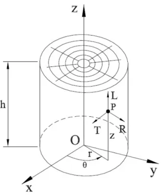
At the macroscopic level, clear wood can be modelled as an anisotropic material. It means that its mechanical behaviour at a given point in the solid, depends on the direction of solicitation. Observing the material structure at the cellular tissue level, three main axes of material symmetry are revealed. These axis defines an orthonormal coordinate system that is typically used in wood and fracture mechanics analysis (Smith et al., 2003). In practice, wood is usually modelled as an orthotropic material with three orthogonal directions (Figure3.6): the longitudinal direction (L), according to the direction of fibers; the radial direction (R), axis perpendicular to the rings of annual growth; and the tangential axis (T), parallel to the rings of annual growth and perpen-dicular to the other two directions of symmetry (Dinwoodie,2000; Kollman and Côté Jr.,1984). These material axes will define three main planes: the transverse plane (RT), the radial plane (LR) and tangential plane (LT). These orthogonal planes are determined through the structure of the wood and the way in which the cells of microscopic structure are arranged (Falk et al.,2010).

3 . 4 . W O O D C H A R A C T E R I Z AT I O N AT H I G H S T R A I N R AT E S

Figure 3.6: Orthonormal material symmetry direction of wood within the stem (Xavier,2003).

3.4

Wood characterization at high strain rates

3.4.1

Intermediate strain rate testing

The range of intermediate strain rates is between 0,01 and 1 s−1and incorporates most possible applications in engineering. For the study of materials subject to intermediate deformation rates, hydraulic servo machines are normally used.

Nakamura et al. in 1980 conducted tests on a shaking table of a one-stage steel structure subject to accelerations, which allowed to conclude that the deformation rates of a seismic event are between 0.01 and 1 sec, range of intermediate strain rates. Therefore, it is relevant to understand the dynamic behaviour of the wood when subjected to intermediate deformation rates, since this biological material is often used for civil construction.

Liska in the year 1950 introduced the concept of duration of load (DOL) and concluded with his scientific research that the tensile strength increases with the decrease of time until the failure of the sample. Subsequently, Liska found that the wood showed a tensile strength 1.26 to 1.28 higher in the static tests than in the dynamic tests for the loading rate that was being used.

Madsen (1975) showed the importance of carrying out tests with samples of structural size, in order to obtain results closer to the properties of the material in its authentic size. After the Madsen reports, the wood science community has implemented more research on structural size samples for this biological material in order to obtain more values for future projects (Polocoser et al.,2017).