An Approach to Earned Value Analysis (EVA): An Application to a Practical Case

(1)

An Approach to Earned Value Analysis (EVA):

An Application to a Practical Case

Maria Isabel Pedro

1

_{, João Pereira}

2

_{, José António Filipe}

3

_{, Manuel Alberto M. Ferreira}

4

1_{Instituto Superior Técnico (IST), CEGIST, Lisboa, Portugal}

Email: ipedro@ist.utl.pt

2

Instituto Superior Técnico, (IST), Lisboa, Portugal Email: ipedro@ist.utl.pt

3_{Instituto Universitário de Lisboa (ISCTE-IUL), BRU/UNIDE, Lisboa, Portugal}

Email: jose.filipe@iscte.pt

4

Instituto Universitário de Lisboa (ISCTE-IUL), BRU/UNIDE, Lisboa, Portugal Email: manuel.ferreira@iscte.pt

Abstract: Nowadays, consumers are becoming more and

more demanding about the quality of the service that are offered to them. To meet these demands, companies do great efforts to offer a high and consistent level for their services. Such an objective can only be achieved if companies have internal capabilities to be, not only effective in delivering what is expected from them, but also efficient in the way their service is performed. It is intended with this work to implement EVA to a specific project using EVA as a methodology.

The main conclusion is that EVA allows a more effective control of the development of projects. It can also be add that good planning and a well-defined organisation of projects are crucial for the quality of the information produced by EVA. It can also be said that EVA must be supported by a very strong method on cost data collecting. On the other hand, EVA has a very strong temporal limitation because it doesn’t take into account the critical path of the project. Therefore, EVA must always be followed by a Gant graph. These conclusions are supported and commentated during this work.

Keywords: Project control, EVA, information systems.

1. Introduction

In an increasingly demanding world, where markets have an extreme competitiveness customer satisfaction is increasingly the central focus of any company that wants to be successful. This satisfaction comes not just from the quality and performance of a product but also from the time/value relationship in its production. It is important to note that today environmental and social concerns are increasing. Thus, a good allocation of resources in order to minimize wastes is considerably important.

For a project’s management to be successfully made, it is necessary the project to be completed within the scheduled time, considering the minimum cost and the best possible quality. In other words, indicators of cost, scheduling, quality, productivity, raw materials consumption and waste may be considered to measure the success of a project. To make possible such analysis, it is necessary to implement a control system. It allows to find discrepancies between what was planned and what was

accomplished. Considering that, the manager will have at this moment all the information necessary to find the causes of the deviations and to implement corrective measures he considers to be relevant.

EVA-Earned Value Analysis is a technique that allows the control evaluation at any time, the performance of time, cost and scope of the project. This means that it compares the planned deadlines for completion of tasks (scheduled work), with tasks actually performed (earned value) from the perspective of planned costs and actual costs incurred. So, the importance of this technique offers an accurate and complete diagnosis of deadlines and costs of a project at any stage of its implementation allowing an efficient supervision and a proper view about its progress.

2. Aim

It is intended to implement EVA to the project SMOPI (this project addresses the main problems in the functioning of the heating and radiation from the pyrolysis furnace and proposes a monitoring system online that will allow very substantially to reduce the consequences of working situations in the transient regime, responsible for the most significant mechanisms degradation in this kind of equipments), by creating a spreadsheet where daily costs incurred by each worker on each task are introduced, in order to make a close and detailed monitoring of the project. This will allow that the results presented by EVA methodology are correct and that the predictions made by this approach are as close as possible to the reality.

3. Methodology

The implementation of EVA to a running project is made. The necessary data are collected through meetings with the team that is responsible for monitoring the projects. If all the data regarding the current development of the project were not available, some assumptions and some scenarios are created in order that the actual EVA model may produce values possible to be interpreted. Follows the analysis and the discussion of the results and yet the interpretation of the possible scenarios created. Finally, the quality of the results and suggestions for a possible implementation of Eva are made.

_________________________________________________________________

International Journal of Finance & Economic Sciences

IJLTFES, E-ISSN: 2047-0916

(2)

4. How to Apply EVA

First of all, in order to apply EVA, it is necessary that the project it is well planned. The project should consist of a list of tasks, with small and manageable work elements easily assigned, monitored and executed. Subsequently, each task must have its start date and its end date well established. Additionally the hours of work that are expected to be spent on each task have to be well defined as well. It is important to collect information such as:

 the precedence in relations among tasks,  the critical path,

 clearances noncritical tasks,  available resources, and to carry out

 risk analysis, and  contingency plans.

EVA is not a tool to be easily used once the project has to be thought out, planned and carried out in a specific structure already outlined for the use of EVA (Wilkens, 1999).

As far as the project is in progress, for using EVA it is necessary to collect, on a regular basis, the information on the real costs and the percentage of completion of each of the tasks. These values are related to the tasks undertaken and completed as well as the ones initiated and not completed since it is assumed that for tasks that have not yet begun, both of these values are zero.

To apply EVA methodology it is necessary, at first, to follow five steps (Wilkens, 1999):

1. Defining the Work Breakdown Structure

(

WBS

)

to divide the project into small chunks, allocating costs to each activity, calculating the required time for each activity and confirming the plan.

2. Identifying the components that compound the activities of the project. The

WBS

provides the framework for identifying the components of the project and each activity has to be associated with an element of the

WBS

.

3. Identifying and allocating costs to each activity. This resource consumption can be expressed in work hours or in monetary units.

4. Calculating the deadlines for each activity (it shows the resources spent on each project phase).

5. Confirming the plan; this confirms the allocation of resources (it is tested if there are the financial and material resources needed to carry out activities in each period of project).

After these first five steps of preparation, it becomes possible to conduct periodic reviews of the project, involving:

1. The update of the calendar, the updating of the progress of the activities.

2. The implementation of the actual costs of each activity.

3. The calculus of the variables of EVA and the preparation of reports.

4. The careful analysis of the variables and the drawing of the necessary conclusions about the project progress.

4.1. Primary Variables

The key variables for the implementation of EVA are presented next:

 The actual Cost of Work Performed (

ACWP

),  The budgeted Cost of the Work Performed (

BCWP

), and

 The budgeted Cost of Work Scheduled (

BCWS

).

ACWP

can be defined as the amount of money spent to finish a task, if already completed, or, as the amount of money spent until the moment, in a given task if it has started but its implementation has not yet been completed. If the project is analyzed as a whole, the ACWP is the total sum of

ACWP

's of all tasks that have already begun, whether they have already been completed or not.

BCWP

is the budget set in the original plan of a task regardless of the money that was actually used to complete it. For a task that has not yet been completed, the

BCWP

is the original budget of the task multiplied by the percentage of completion of a specific task until the moment considered.

BCWP

is the total sum of the

BCWP

for all tasks that have already begun, whether these have been completed or not.

BCWS

is the monetary value that was supposed to be spent on tasks that were expected to completed by then. For tasks whose completion should have been reached,

BCWS

is the budget of the original task, whether it is actually completed or not. For tasks which implementation should have been started but not completed,

BCWS

is the original budget of the task multiplied by the percentage that is expected to perform it until the date considered. As with previous variables, the total

BCWS

is the sum of the

BCWS

for all activities.

It should be noted that these three variables are in fact functions of time, either for individual tasks or for the project as a whole, and must be recalculated whenever the model applies EVA. This observation is easily understood since, as time passes, more money is spent, more work is done, and the simple advance of time makes that what is expected to be spent and what is expected to be achieved are successively changing (Cesarone, 2007).

4.2. Secondary Variables

Once calculated the primary variables, ie, the

ACWP

, BCWP and BCWS either for tasks that should have begun by the date in question, either for the overall project, it is time to calculate the value of the secondary variables.

Scheduled Variance (

SV

) compares the progress made with the expected progress, dividing this difference

(3)

by the expected progress. Thus, it provides information on the percentage of variation or deviation from what had been previously planned. This variable can be calculated by the following expression:

BCWP BCWS

SV

BCWS  

If

SV

is positive, the activity that is being examined is ahead of what was previously expected. If not,

SV

has a negative value and the activity is delayed.

On the other hand, Cost Variance (

CV

) compares the incurred cost with the planned cost of the tasks that were actually carried out. The normalization of this value is done by dividing the planned cost for the percentage of deviation from the original plan. The expression for calculating this variable is

BCWP ACWP

CV

BCWP  

If

CV

is positive, the activity in question may have had a lower cost than the forecasted. On the contrary, if

CV

shows a negative value, the task has exceeded the budget until the date in question.

Another variable which interpretation may be relevant is time change, or Time Variance (

TV

). This variable is the difference in time between the earned value (

BCWP

) and the planned value (

BCWS

).

Continuing a temporal analysis, the final variation of the terms, or Delay at Completion (

DAC

), is calculated as the difference between the projected date for completion of the project (

TAC

- Time at Completion) and the date initially planned for the end of the project

(PAC

- Planned at Completion). Thus the following expression can be used:

DACTACPAC

By turn, Scheduled Performance Index (

SPI

) gives a relationship between

BCWP

and the planned value (

(

BCWS

)

in a given date.

SPI

shows the conversion rate of the predicted value in earned value, up to that date, and can be calculated using the following formula:

BCWP SPI

BCWS 

For a better understanding of

SPI

concept, consider

0.9 SPI



. This means that 90% of the budgeted time was converted into work. Thus, it is apparent that there was a 10% loss in the available time. One can then

generalize by saying that if the value of

SPI

is equal to 1, the planned value was fully added to the project. Following the same logic, a SPI value of less than 1 indicates that the project is delayed and a value of more than one SPI, that it is advanced.

Another ratio which analysis can also be quite indicative of the project progress is the Cost Performance Index (

CPI

). Here a relationship between

BCWP

and actual cost of the project (

ACWP

) is given.

CPI

shows the rate between the actual consumption and the aggregate values in the same period and may be calculated using the following expression:

BCWP CPI

ACWP 

If

CPI



0.9

is considered, this means that for every €1 of capital consumed, only 0.9 € are in fact being converted to final product and, as such, there is a loss of 0.1 € per each 1 € spent. Again, a

CPI

value equal to 1 indicates that the amount spent by the project was completely earned and, as such, the project is within budgeted. If

CPI

is less than 1, the project is spending more than expected and there will probably be an extra cost at the end of it. Similarly, if the

CPI

is greater than one, the project is to cost less than budgeted.

For each time EVA is recalculated, it is important to determine the Estimate at Completion (

EAC

). This variable informs about the expected evolution of the project costs and the fact that such a measure can be determined is one of the great advantages of EVA. The value of

EAC

can be calculated using the following formula: BAC BCWP EAC ACWP CPI   

To use this formula some assumptions have to be accepted. Firstly, the current cost of the project must be greater than planned, for work already performed

(

ACWP



BCWP

)

. Thus, if costs continue this trend, it is easy to see that the estimated cost at the end of the project

(

EAC

)

will be much higher than budgeted at Completion -

BAC

on this date. Thus, the

EAC

formula represents the work that it is not yet been completed

(

BAC



BCWP

)

, dividing it by the

CPI

. Later, the cost of work completed (ACWP) is added, which is seen as a sunk cost.

Finally, it is possible to calculate the Variation at Completion

(

VAC

)

by subtracting the

EAC

to

BAC

, as it is showed by the following expression:

(4)

The list of secondary variables is based on the "paper" prepared by Giacometti et al (2007).

4.3. How to Improve EVA Performance

As it was seen earlier, EVA is a very efficient and useful technique to evaluate a project’s performance. However, it still has some flaws which reduce its applicability. In order to eliminate these flaws, Rodney Howes, a professor at the University of South Bank, London, conducted a study which develops a hybrid approach that attempts to answer such faults.

In fact, traditional EVA evaluates the cost performance using the Cost Variance

(

CV

)

and Cost Performance Index

(

CPI

)

which gives a very useful measure unit. However, the Estimated Cost to Completion

(

ECC

)

and Forecast of Project Completion Cost

(

FCC

)

are based on past performance, and often, this is incorrect because the future work can be quite different from the one already done. Another limitation of EVA is that the Scheduled Variance

(

SV

)

is purely related to the performance of cost and does not take into account the time related to the completion of tasks in their logical sequence. This is a very serious limitation because the cost is not directly proportional to time. Finally, in its most basic version, EVA does not take into account variations in the project in the form of additions or omissions.

Being aware of such faults, Howes (2000) developed a methodology for cost and schedule that can give a better, and more robust and reliable analysis of the project which is called Work Package Method

(

WPM

)

. This new methodology considers the project as a set of small inter-related packages on time and sequence. These packages are classified as completed, under way or about to start. The occurrence of variations to the initial project budget

(

BCWS

)

could be identified and taken into account. Thus, the omissions would be deducted and their effect over time would be counted. The additions would be computed and compiled as identifying factors. Thus, delays caused by changes to the packages would be evident.

Howes (2000) has in fact refined and improved the performance of traditional EVA to introduce a hybrid approach based on work packages and temporal logic analysis to which he gave the name of

WPM

. This tool allows to regularly update the project cost and its time performance restricting the calculation of EVA to individual packages.

5. Case study – Project SMOPI

The main objective is the implementation of EVA model to the SMOPI project, which is still in development.

As with any project, there is a list of activities by which the project is developed. In the case of SMOPI, the list of activities is as follows in fig 1.

Figure 1- List of Activities - SMOPI

1 Preliminary studies 2 Techniques specifications

3 Acquisition and development of new knowledge 4 Development

5 Construction of prototypes, pre-sets and experimental setup

6 Tests

7 Promotion and disclosure of results

Each of these activities consists on tasks to be accomplished. In its simplest form, these tasks are mini-objectives, "milestones" to be achieved at all times.

6. Implementation of EVA

Now is holding up the implementation of EVA model to the SMOPI project. To simplify the calculations, the values of "overhead" were not taken into account.

6.1. First Point of Control - 3 months

EVA is a project control methodology and as such, tracks progress and makes forecasts for the project. Doing this first test three months after the start of the project, it is always necessary to calculate the expected scenario, according to the forecasts and to the previously planned and the real scenario.

6.1.1. Estimated Situation

According to the original timetable, at 3 months, the situation should be:

Table 1 - Predicting SMOPI - 3 months

Tasks performed

Performed status (Forecast)

1.A - Study of Hardware Installation in

the Furnace 100%

1.B - Study of System Acquisition,

Storage and Data Transfer 25%

1.C - Model Study of Coking 50%

Analyzing the form, it is possible to know the cost of each task:

(5)

Table 2 – Description of task 1A Technical Staff Code Technical Staff Name Hours Worked (h) Cost by hour worked Total 0.1 José 45 34,74 € _{1.563,30 €} 0.2 Carlos 30 25,13 € _{753,90 €} 0.3 Ivo 120 26,31 € _{3.157,20 €} 0.4 Rui 55 26,31 € _{1.447,05 €} 6.921,45 € Technical Sub- contractors Employee sub-contractor name Hours Worked (h) Cost by hour worked Total Matos 25 70,00 € 1.750,00 €

Table 3 – Description of task 1B

Technical Staff Code Technical Staff Name Hours Worked (h) Cost by hour worked Total 0.1 José 285 34,74 € _{9.900,90 €} 0.3 Ivo 212 26,31 € _{5.577,72 €} 0.6 Rui 212 19,71 € 4.178,52 € 19.657,14 € Technical Sub- contracto rs Employe e sub-contracto r name Hours Worked (h) Cost by hour worked Total Matos 40 70,00 € 2.800,00 €

Table 4 – Description of task 1C

Technical Staff Code Technical Staff Name Hours Worked (h) Cost by hour worked Total 0.3 José 145 26,31 € _{3.814,95 €} 0.4 Rui 355 26,31 € _{9.340,05 €} 1.1 Pedro 35 32,93 € _{1.152,55 €} 1.2 Luis 140 21,99 € _{3.078,60 €} 1.4 Celso 75 26,81 € _{2.010,75 €} 1.6 Nuno 130 16,96 € _{2.204,80 €} 1.9 Manuel 285 22,58 € _{6.435,30 €} 1.10 Sandra 305 15,58 € 4.751,90 € 32.788,90 € Technical Sub- contracto rs Employe e sub-contracto r name Hours Worked (h) Cost by hour worked Total Matos 20 70,00 € 1.400,00 €

At this point, the cost of each task and its degree of progress is known. It is possible to calculate now how much it should have been spent on each task at 3 months and therefore how much it should have been spent in total: Cost of task 1A (forecast) Cost of task 1B (forecast) Cost of task 1C (forecast) 8.671,45 € 5.614,29 € 17.094,45 € Total Estimated Cost 31.380,19 €

6.1.2 Real Situation

At this moment, the real situation regarding the project is according the following:

• Task 1A was more difficult than originally thought so the technicians have dedicated over 5% of their time to it so that it was finished on time.

• Due to technical problems, the task 1b delayed 1 month. The control at 3 months had not yet started. This event causes that 2.B and 4B are also delayed one month.

• Task 1.C has delayed one week its start making that 3.C and 4.C also are delayed one week.

Given these assumptions, the scenario for three months is as follows:

Table 5 – SMOPI Real Situation– 3 months

Tasks Performed Performance

Status (Real) 1.A - Study of Hardware Installation

in the Furnace 100%

1.B - Study of the Acquisition

System, Storage and Data Transfer 0%

1.C - Study Coking Model 46%

As the task 1A will be more expensive because workers have spent more hours than anticipated, the task 1B has not yet begun; and task 1C is one week late. The actual costs of the tasks are:

Cost of Task 1A (Real) Cost of Task 1B (Real) Cost of Task 1C (Real) 9.105,02 € 0,00 € 15.669,91 €

Total Estimated Cost 24.774,94 € As can be seen after 3 months from the start of the project, in the project an amount of 6,605.25 € is spent less than the expected. However, is it a good sign? In fact, more work may have been developed or a lesser amount of spending made than the expected, to make the same quantity of work. However, often this is not the case. A lesser amount of money spent than the expected may indicate that the project is delayed and, as such, the amount spent is not the amount that was owed to be spent .

Let's apply EVA variables and see the conclusions.

6.1.3. Calculation of EVA Variables and First

Conclusions

The application of the following formula is made with respect to each of the tasks that now should have been completed or initiated. Then, it is the same analysis for the project as a whole:

(6)

Table 6 - Primary and Secondary Variables - Task 1A ACWP 9.105,02 € BCWP 8.671,45 € BCWS 8.671,45 € Schedule Variance (SV) 0 Cost Variance (CV) -0,05

Scheduled Performance Index (SPI) 1

Cost Performance Index (CPI) 0,95

As can be seen,

ACWP

is greater than

BCWP

, indicating that it is spending more than expected. This is evidenced by a negative

CV

or a

CPI

lesser than 1, i.e. the task 1A, from each € 1 of capital consumed just 0.95 € are converted into the final product.

On the other hand,

BCWP

is equal to

BCWS

indicating that the task did not deviate temporarily from what has originally been planned. This is clearly visible by an

SV

equal to 0 or an

SPI

equal to 1.

It may seem strange that BCWS is equal to

BCWP

since a greater amount was spent than the expected. However, when a task is completely full, its

BCWP

is equal to what had been planned (

BCWS

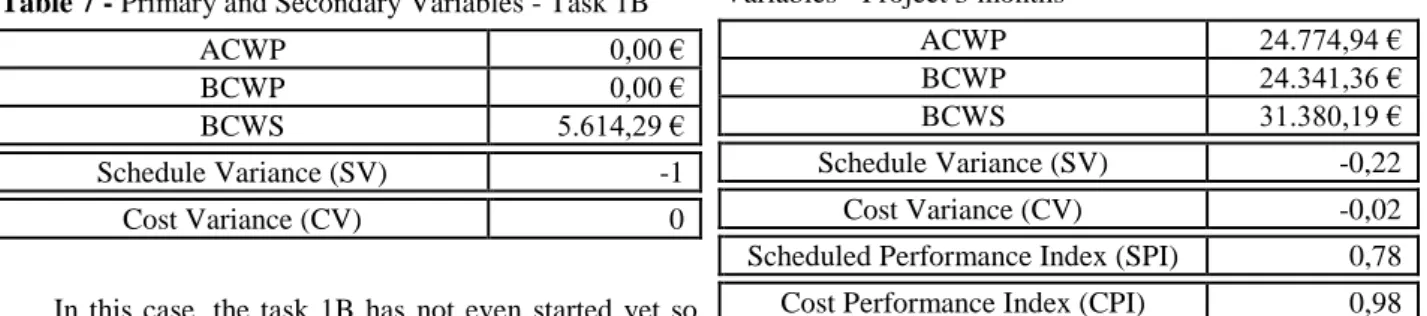
), although it has been spent a greater or a lesser amount. It is for this reason that the implementation of EVA requires not only that the project has been conceived and structured by tasks for a possible implementation of EVA, but it has been thought by people with great experience because, as can be seen, initial estimates are very important and determine the purchased value.

Table 7 - Primary and Secondary Variables - Task 1B

ACWP 0,00 €

BCWP 0,00 €

BCWS 5.614,29 €

Schedule Variance (SV) -1

Cost Variance (CV) 0

In this case, the task 1B has not even started yet so there was no spent money. In fact, as

SV

has a negative value the task is overdue, but as

SV

is equal to -1 this means that the task is not only delayed but also it has not started yet. It is understood also that

CV

is equal to 0 because the task has not started yet, there was no spent money yet and, consequently, there cannot be any deviation.

Table8-Primary andSecondaryVariables-Task

1C

ACWP 15.669,91 €

BCWP 15.669,91 €

BCWS 17.094,45 €

Schedule Variance (SV) -0,083

Scheduled Performance Index (SPI) 0,92

Cost Performance Index (CPI) 1

In Task 1C,

ACWP

equals

BCWP

and

consequently,

CV

is equal to 0 and

CPI

is equal to 1. In fact, the money spent is exactly what was intended to spend.

On the other hand,

BCWP

is lesser than

BCWS

and this is visible because

SV

is negative and

SPI

lesser than 1. In this case, 92% of the expected budgeted time was converted into work, so there was an 8% loss in the time available.

In fact, if it is only compared

ACWP

and

BCWS

, it is possible to make the mistake of saying that the amount spent could be lesser than the expected. This would be great. For this reason, there is a variable

BCWP

, or acquired value. The ideal situation would have

BCWP

greater than

BCWS

, indicating that the task would be advanced and an

ACWP

lesser than

BCWP

, indicating that a lesser amount is spent than what was due to the percentage of work performed.

Following this analysis for all the tasks separately, it is possible to do the following analysis for the project as a whole:

Table 9 - Project – Overview - Primary and Secondary

Variables - Project 3 months

ACWP 24.774,94 €

BCWP 24.341,36 €

BCWS 31.380,19 €

Cost Variance (CV) -0,02

Scheduled Performance Index (SPI) 0,78

As can be seen, this is the worst possible scenario. The project not only is delayed as it is spending more than the expected. Although EVA shows that the project, at this time, is late, it is not possible to inform if the project will be delayed when it is complete. For this reason, it is always necessary to monitor the implementation of EVA with a Gant chart, or any other graphics where are visible the precedence between tasks, to understand if the delays which occur at some point will affect the scheduled completion date of the project. The Gant chart complements the EVA and allows to verify if delays occur in the critical tasks (automatically delaying the project) or in secondary tasks. Even if there is the

Cost of task 1A (real) Cost of task 1B (real) Cost of task 1C (real) 9.538,6 € 0,00 € 14.245,38 €

(7)

second case, if the delays are greater than the gaps of these tasks, the project also delays.

The final budget forecast

(

BAC

)

is € 1,082,348.88. Calculating

EAC

a value of € 1,101,627.86 is obtained. Although EVA cannot predict whether the project will be late, informs that supported on this trend the project will cost more € 19,278.98 (

VAC

) than initially budgeted.

6.1.4 Sensitivity Analysis

In order to examine how EVA performs facing different situations of different severity, sensitivity analysis will be made now. So, and assuming the same assumptions created for this control point at 3 months, two scenarios will be discussed:

• A first scenario where the observed failures are more severe (the task 1.A requires more 10% of workers time, the task 1.B has not still started and the task 1.C is 2 weeks delayed)

• A second more optimistic scenario (task 1A requires only 1% of the workers time, the task 1.B has not still started and the task 1.C is just 1 day delayed). Applying the first scenario, i.e., exacerbating the initial assumption conditions, the real new costs of € 23,783.97 for new tasks, and the new total costs spent are: In this case, an amount of € 7596.22 is spent lesser than the expected and lesser € 990.97 than the situation described in the scenario with the initial assumptions. Looking more closely each task, it can be seen that

CV

of task 1A is replaced by a

CV

equal to -0.1 and a

CPI

equal to 0.91. This kind of values was expected because the costs of this task were all enhanced in the same scale. For its part, the

SV

of task 1.C is replaced by a

SV

equal to -0.167 and a

SPI

of 0.83. These values are also expected because the delayed time was twice the one expected on the initial assumptions. However, looking at the project as a whole, it appears that the

EAC

is equal to € 1,123,303.66, and so, the project will cost more € 40,954.8 than originally planned. If this value is compared to the

VAC

obtained for the initial assumptions (€ 19,278.98), it can be seen that there is a slight worsening of the situation. In fact, it was expected to spend more because the conditions were worse than the other situation but EVA does not convey this information in a linear way. The worse the situations are, the worst are the estimates provided by EVA.

Let's see if this trend continues for the most optimistic scenario. The values of the tasks are:

Cost of task 1A (real) Cost of task 1B (real) Cost of task 1C (real) 8.758,16 € 0,00 € 16.752,56 €

Total Estimated Cost 25.510,73 €

As expected, the cost of task 1A is very close to the estimated cost as the workers are working only 1% more than the allotted time. Simultaneously, the cost of the task 1.C is also very close to the estimate because the task is

49% while provisionally would be 50%. Obviously, the actual cost at this point deviates a bit more than expected because the task 1.B still has not been started.

Looking at the project as a whole, it appears that the

EAC

takes the value of € 1,086,040.48, only € 3691.60 more than was initially expected. In fact, EVA is a tool sensitive to the deviations, not dealing with these variations in a linear way. Simplifying a little the following statement, it can be said that EVA comprises more than € 1 spent today could mean spending more than € 2 at the end; but spending more € 2 may mean spending more than € 5 or € 6 at the end. The worse the present conditions are, the worse are the forecasts provided by EVA.

6.2 Second Point of Control - 12 months

Next, the same analysis made earlier will be held but at 12 months from the start of the project. Note that it is imperative to update calendar whenever it is applied EVA, i.e., to make this analysis at 12 months, the timetable should be the one after the control at 3 months (A.3) and not the original. In fact, over the costs of the tasks, updating the calendar or not has no impact. However, in relation to timings is easy to understand why there is a need to update the calendar. Imagine, for example, that a project delayed in the first month but then will not delay anymore. If an inspection after the first month of work is made, in fact, it is possible to ascertain that the project is delayed. However, unless the schedule is updated when we return to do a checkpoint, the result will be that there is yet a delay. That is, if one reads the report he can think that tasks have delayed again, when in reality the tasks are progressing at the pace that was predicted but were late in the first month.

6.2.1 Estimated Situation

According to the updated timetable after 3 months (A.3) control, the theoretical situation is as follows:

Table 10 - Expected SMOPI - 12 months

Tasks Performed

Performanc e Status (forecast) 1.A - Study in the Furnace Installation

Hardware 100%

1.B - Study System Acquisition, Storage

and Data Transfer 100%

1.C - Model Study of Coking 100%

1.D - Study Model Carburetion 67%

1.F - Study of Creep Damage Model 33% 2.A - Technical Specification of

Hardware Installation in the Furnace 100%

2.B - System Specifications 100%

3.C - Pre-Development Model Coking 100% 4.B - Development of the Acquisition,

Storage and Data Transfer 60%

4.C - Model Development Coking 22%

5.A - Prototype Hardware Installation in

(8)

6.A,B,C - Field Tests (Since we're halfway through the year 2010, it is assumed that half hours were spent in this task)

Following the same reasoning used to calculate the theoretical costs of these tasks, it is possible to come to the following values:

Cost of Task 1A(Forecast) 8.671,45 € Cost of Task 1B(Forecast) 22.457.14€ Cost of Task 1D(Forecast) 18.439,17 € Cost of Task 1F(Forecast) 35.194,79 € Cost of Task 2B(Forecast) 29.584,45 € Cost of Task 3C(Forecast) 21.933,95 € Cost of Task 4C(Forecast) 9.446,95 € Cost of Task 5A(Forecast) 13.580,22 € Cost of Task 1C(Forecast) 34.188,90 € Cost of Task 2A(Forecast) 10.207,50 € Cost of Task 4B(Forecast) 22.527,81 € Cost of Task 6A,B,C (Forecast) 9.395,49 €

Total Cost (expected) 235.627,81 €

Keeping the events that were manifested at 3 months, the new records are now:

•Task 1.D delays its start in three months and, to try to compensate the lost time, workers work 10% more time than the expected.

•Tasks 2.B and 5.A used less than 5% of the expected time.

Given these assumptions, the scenario for 12 months is as showed table11.

Table 11 - Real Situation SMOPI - 12 months

Tasks

Performed Performance Status (Real)

1.A 100% 1.B 100% 1.C 100% 1.D 33% 1.F 33% 2.A 100% 2.B 100% 3.C 100% 4.B 60% 4.C 22% 5.A 100%

6.A,B,C Took up half of hours spent

Again, taking into account the changes in the percentage of tasks completion and hours spent by workers, the real costs are:

Cost of Task 1A (Real) 9.105,02 € Cost of Task 1B (Real) 22.457,14 € Cost of Task 1D (Real) 10.040,13 € Cost of Task 1F (Real) 35.194,79 € Cost of Task 2B (Real) 28.105,23 € Cost of Task 3C (Real) 21.933,95 € Cost of Task 4C (Real) 9.446,95 € Cost of Task 5A (Real) 12.901,21 € Cost of Task 1C (Real) 34.188,90 € Cost of Task 2A (Real) 10.207,50 € Cost of Task 4B (Real) 22.527,81 € Cost of Task 6A,B,C (Real) 9.395,49 €

Total Cost (Real) 225.504,11 €

Again, the amount spent is € 10,123.79 lesser than the expected. This applies to EVA variables on each task separately and subsequently to the project as a whole.

6.2.3 Calculation of EVA Variables and Conclusions

Although it is necessary to calculate all variables for all tasks, here it will be presented only the most relevant. In this case, they are the tasks 1D and 2B:

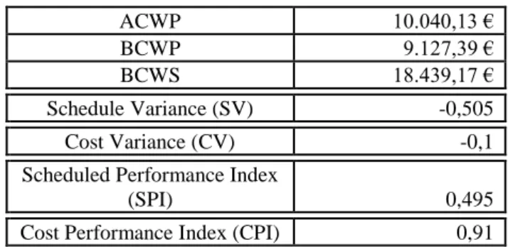
Table 12 - Primary and Secondary Variables - Task 1D

ACWP 10.040,13 €

BCWP 9.127,39 €

BCWS 18.439,17 €

Cost Variance (CV) -0,1

Scheduled Performance Index

(SPI) 0,495

In this case, the task is behind schedule (

SPI

lesser than 1) and spends more than expected (

CPI

lesser than 1). As this task is not finished yet, the

BCWP

is lesser than the

BCWS

once the task is delayed (and thus cost more). However, if the task was already completed,

BCWP

would be equal to

BCWS

, even if the task is behind schedule and had cost more because

BCWP

is the purchased value. Again, it is important to have a good planning, made by someone experienced and preferably with knowledge on the application of EVA.

Table 13 - Primary and Secondary Variables - Task 2B

ACWP 28.105,23 €

BCWP 29.584,45 €

BCWS 29.584,45 €

Schedule Variance (SV) 0

Cost Variance (CV) 0,05

Although 2B is late due to a delay in 1B, this task has been completed so that its SPI is equal to 1.

(9)

On the other hand, as would be expected, CPI is greater than 1, indicating that the amount spent is lesser than the expected.

Finally, the project is analyzed as a whole:

Table 14 - Project - Overview Primary and Secondary

Variables - Project 12 months

As can be seen through this analysis, the project is behind schedule (

SPI

lesser than 1) but has spent lesser than was originally expected (

CPI

greater than 1). Also noteworthy is that the same analysis was done at 12 months but with no update schedule. As it was expected, SV gave a more negative value and

SPI

a less positive value. This is because, to update the schedule, it is already known that 4B and 4C are going to delay (hence no longer delays). In fact, on this analysis at 12 months, only the delay of 1D was not foreseen and the values of SV and SPI shows that.

In this case, the

EAC

is € 1,078,465.89 which shows that, supported in this trend, an amount of less € 3,882.99 was spent than the originally planned.

6.3 Third Point of Control - 18 months

Following the same reasoning used in the previous analysis and updating the calendar with the changes at 12 months (A.4), it is not necessary to present the theoretical situation. It is easily calculable. It is noteworthy that on this date it was expected that an amount of € 400,615.45 was already spent. Again, if the calendar was not updated, this value would be greater because there would be to take into account the delays that have already occurred and others that are allowed to be anticipated, thus no longer be considered delays, or rather, they are delays but they are expected delays.

Keeping the scenario that was manifested at 12 months, the new records are now:

•Tasks 1.E and 1.F began on schedule but are now one month late because each employee spent less 3% than the time that they should.

Given these assumptions, the scenario for 18 months is as follows:

Table 15 - Real Situation SMOPI - 18 months

Tasks

Performed Performance Status (forecast)

1.A 100% 1.B 100% 1.C 100% 1.D 100% 1.E 86% 1.F 90% 2.A 100% 2.B 100% 3.C 100% 4.B 100% 4.C 97% 5.A 100%

6.A-H (As this is the end of the year all hours are appointed for this task 9)

Note that the task 1E should be complete all the 6 months of the planned 6. As the task has begun on schedule but it is lasting more one month, there are 6 complete months of the 7 that the task will take in reality. The same reasoning may be applied to 1F.

Thus, applying the same reasoning used here to calculate costs for each task, the actual cost is € 383,430.53, i.e., less € 17,184.91 than what was estimated.

Again, the calculations are presented only for the tasks most relevant:

Table16 - Primary and Secondary Variables - Task 1E

ACWP 23.757,99 €

BCWP 24.492,77 €

BCWS 28.574,90 €

(SPI) 0,86

ACWP 225.504,11 €

BCWP 226.316,03 €

BCWS 235.627,81 €

Scheduled Performance Index (SPI) 0,96 Cost Performance Index (CPI) 1,0036005

(10)

Table17 - Primary and Secondary Variables - Task 1F ACWP 92.175,16 € BCWP 95.025,93 € BCWS 105.584,37 € Schedule Variance (SV) -0,1 Cost Variance (CV) 0,03

(SPI) 0,9

Once both tasks 1.E and 1.F follow the same standard, the following analysis is valid for both. How

ACWP

is lesser than

BCWP

, the task is spending less than expected (a good result). How

BCWP

is lesser than BCWS, the tasks are overdue (bad news). The ideal situation would have

BCWP

greater than

BCWS

, i.e. would be advanced, and

ACWP

lesser than

BCWP

, i.e., spending lesser than expected for that level of achievement.

Analysing the project as a whole, it is possible to have now:

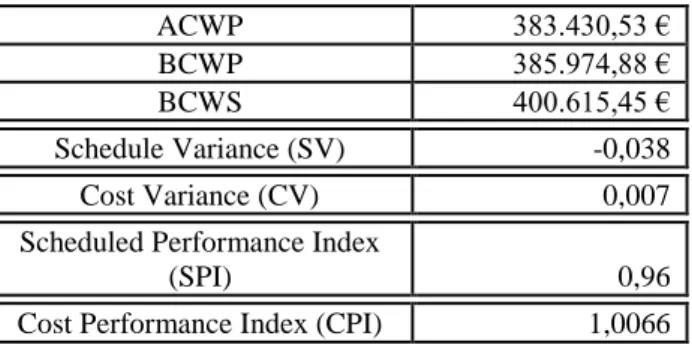
Table 18 - Project - Overview Primary and Secondary

Variables – Project 18 months

ACWP 383.430,53 €

BCWP 385.974,88 €

BCWS 400.615,45 €

(SPI) 0,96

As shown, the project continues to delay (96% of the expected time budgeted was turned in work which results in a loss of 4% in the time available) but spend less than expected (for each € 1 of capital consumed, € 1.0066 being physically converted into work).

In this case, the

EAC

is € 1,075,214.03, i.e., EVA provides that at the end of the project are spent € 7134.85 less than expected.

6.4 Fourth Point of Control - 36 months

This control point is made upon the completion of the project, or better, on schedule for completion of the project.

Following the updated timetable for the control after 18 months (A.5), the expected total cost for this project is € 686,888.08. In fact, the cost will be the

BAC

, i.e. € 1,082,348.88 as reported earlier but was not taken into account the overheads or any item regarding the purchase of equipment.

Although it is not considered any further changes until the end of the project, the delay already occurred in 1F causes delays in 4F and, so, it also delays the project, which will last 37 months. In this case, the actual cost of the project in this date is € 683,904.51.

Again it is spending less than expected but does EVA confirm that this is a good sign?

Calculating EVA variables for task 4F:

Table 19 - Primary and Secondary Variables - Task 4F

ACWP 48.539,29 €

BCWP 48.539,29 €

BCWS 48.539,29 €

Cost Performance Index (CPI) 1

Despite being the only task that has not been completed and to be delaying the project in one month, it was already known that this would happen due to updated calendar that was performed at 18 months. As such, this task is not delayed in accordance with that update, it is relating the initial expectation.

Table 20 - Project - Overview Variables Primary and

Secondary - Project 36 months

ACWP 683.904,51 €

BCWP 686.888,08 €

BCWS 686.888,08 €

From 18 months timetable until now there has not been any change in tasks. As such, it was expected that no change in the schedule would occur, as shown by the SPI.

CPI is greater than 1, which indicates that the project is costing less than expected. For each € 1 of capital consumed, € 1.00436 are being converted to physically work.

Knowing that the

BAC

was € 1,082,348.88, and that in time, the

EAC

is € 1,077,647.59, the

VAC

is € 4,709.29, i.e., the project will cost less than initially expected. In fact, since the 18 months so far no work has changed. At 18 months, there was a tendency for tasks

(11)

costing less than expected and, so, was expected to spend less than € 7,134.85 which had been originally planned. In these second 18 months, the tasks were not affected so, the tendency has been blurred. As such in the end of the project it will pay € 4701.29 less than expected.

7. Conclusions

EVA is a methodology for project control and, so, should monitor their implementation. Naturally, the often the application of EVA and the less times passes between two applications more reliable will be the results and more timely may be detected failures and delays to take appropriate action.

EVA is not a tool of easy use and its implementation has costs, namely a platform to collect the costs associated with the project but also costs of personnel training. It is important that initially is resorted to the services of someone experienced in the implementation of EVA, not only because the tool itself, which has some nuances, but also because the project planning itself is critical to the success of EVA.

In this kind of analysis, EVA provides interesting information and conclusions. In fact, if a project is spending less than the expected, and assuming that the forecasts are good, this is not synonymous of a good performance. As shown in the EVA application, the task is often delayed and there is therefore not yet spent what was expected. On the other hand, as the name shows, EVA is based on the value purchased. For this reason, the planning and initial forecasts are so important, because even if a job cost more or less, when it ends, its acquired value is what it is initially planned and not the final value. Through a sensitivity analysis performed at 3 months, where it was considered a worst scenario and a best scenario, it was found that EVA is sensitive to changes not only in relation to what was initially expected but also in the severity of these changes. In other words, this sensitivity analysis showed that the additional costs are exponential throughout the project. As such, a small variation in the costs incurred will be reflected in a small variation in the final cost of the project but a variation, for example, 5% higher, will not reflect on just 5% at the end of the project. This amount would be higher because this trend of cost is not linear.

It is also important to note that EVA is not about to make good estimates and to obtain data about the progress of various tasks (which can also be difficult if the staff is not accustomed to providing such information regularly). In fact, having data on current costs may also become a problem because many companies report their cost reports with several weeks of delay. Moreover, the cost of a required equipment for the project may not appear in official accounts of the company but this money is as if he had already been spent. As it is visible, there are many variables that can influence the results of EVA, fudging them.

Some repairs on the EVA tool.

EVA is a tool difficult to implement and, so, or the company already has an high organization and has a good computer system that allows to effectively manage the costs incurred or so the results do not reflect correctly what happens in reality.

EVA does not take into account the critical path. That is, as noted earlier, there are formulas that calculate time deviations and can even make predictions about the end date of the project. However, if a non-critical task is delayed one day (and has a margin), EVA will inform that the project will also be delayed (not necessarily the same one day). In fact, this is not true and that is why it is suggested that, parallel to the use of EVA, it is necessary to build Gant diagrams or even to do a critical path analysis as a way to fill this gap. As such, and because of this failure, may not make sense to calculate, at each checkpoint, the

SV

and

SPI

for the project in general. In fact, these variables calculated for each task individually provides information about their progress and if they are delayed or not. However, translating them for the project in general lays bare this limitation of EVA because, again, any delay in any task, however small it may be, will be reflected in a delay of the project and this may not be true.

The EVA does not identify the reasons for delays in the schedule or to variations in costs and has no ability to suggest corrective measures.

Finally, why may EVA be used? In fact, the main reason is to provide numerical data to the manager so that he can effectively monitor the project. However, if thought in a less rational and more emotional way, it is understood that nobody likes to see that he has had bad results. If the information obtained through EVA is published, everyone will work harder as a way to obtain better performances and a way to motivate all the personnel involved in the project.

References

[1] Wilkens, T. T., Earned Value, Clear and Simple,

Metropolitan Transportation Authority, Los Angeles CA (Currently with Primavera Systems, Inc.) April 1, 1999.

[2] Cesarone, J., Project Management by the numbers –

How earned value analysis can keep you on track,

Industrial Engineer-Norcross, Boyd & Goldratt, 2007.

[3] Giacometti, R. A., Silva, C. E. S., Souza, H. J. C., Marins, F. A. S. e Silva, E. R. S., Aplicação do Earned Value em projectos complexos – um estudo de caso na Embraer , Gest. Prod., São Carlos, v. 14, n. 3, p. 595-607, set.-dez., 2007.

[4] Howes, R., Improving the performance of Earned Value Analysis as a construction project management tool”, Wiley, Engineering Construction and Architectural Management Volume 7, Issue 4, pages 399–411, December,