A Work Project, presented as part of the requirements for the Award of a Master Degree in Finance from the NOVA School of Business and
Economics.
On the value of European options on a stock
paying a discrete dividend at uncertain date
Jos´e Ant´onio Gomes de Sousa Pereira n 2408
A Project carried out on the Master in Finance Program, under the supervision of
Jo˜ao Amaro de Matos
On the value of European options on a stock paying a
discrete dividend at uncertain date
Abstract
The purpose of this paper is to evaluate the impact of uncertainty about the dividend date on the value of European options in the context of the Black-Scholes model. We use an arbitrarily accurate numerical approxima-tion for the value of this type of instrument on a stock paying a discrete dividend, considering different probability distributions over the date of dividend payment, and comparing with the deterministic case. We find that the main determinant is the skewness of the probabilistic distribu-tion. For positive skewness, uncertainty about the dividend payment day decreases the value of the option, and negative skewness has the oppo-site effect for standard parameters. However, if interest rates are negative, volatility is small enough and the option is sufficiently in the money, the impact of uncertainty is reverted. The understanding of this mechanism may have practical implications for hedging strategies.
Keywords: European Options, Discrete Dividends, Uncertain Ex-Dividend Date.
1
Introduction
Valuing a simple European option under the Black-Scholes (1973) model has a closed form solution. To solve it, the distribution for returns of the stock on which the option is written is assumed to be log-normally dis-tributed as seen from the emission time. However, if a discrete dividend is included during the life of the option, the stock jumps at the dividend pay-ment and the log-normal assumption is no longer valid. As a consequence, the Black-Scholes closed-form solution is no longer applicable.
There are several approximations to value one such option, the most common of which is the escrowed dividend model first suggested by Black (1975) and discussed by Roll (1977). Under this approximation the present value of the dividend to be paid is subtracted from the initial price of the underlying asset and the Black-Scholes formula is applied.
Other more efficient approximations have been suggested. Beneder and Vorst (2001) proposes that the volatility input for the underlying asset to be set as a weighted average of two variances (one before the dividend, and another after), where the weighting values depends on how late in the life of the option the dividend is paid.
Although brute-force methods such as Monte-Carlo simulations can make extremely good approximations with a well-characterized error dis-tribution, they are relatively slow, as they require a lot of computational time.
Amaro de Matos et al. (2009) introduces a quasi-analytical method to accurately approximate the value of European options that pay a single discrete dividend. This method is based on the calculation of an upper and a lower bound for the value of the option that quickly converge. The objective is to set the difference between those bounds sufficiently close to 0. The equations for these bounds were analytically obtained by using the convexity properties of the Black-Scholes option pricing formula.
the impact of skewness on the value of the option is reverted.
This paper is organized as follows. In the following section we present the methodology. Next we present the results, first with fixed parameters, and then developing a sensitivity analysis on how the results depend on these parameters. Finally we discuss the results and present our conclu-sions.
2
The Methodology
In this paper all the values of European options paying a discrete divi-dend are calculated using the method developed in Amaro de Matos et al. (2009). We introduce below the resulting upper and lower bounds for the options:
Upper bound:
V(S,0)≤U P =
M
X
i=1
[aiAiS+e−rtD[V(Si−1, tD)−aiSi−1]Bi]
+SN(d∗
1) +e−rtD[V(S∗, tD)−S∗]N(d∗1 −σ
√
tD)
Lower bound:
V(S,0)≥DOW N =S
M
X
i=1 V′(S
i+1
2, tD)Ai
+e−rtD
M
X
i=1
( [V(Si+1
2, tD)−V
′(S i+1
2, tD)Si+ 1 2]Bi)
+SN(d∗
1)−e−rtD[D+Ke−r(T−tD)]N(d∗1−σ
√
tD)
where
ai = S∗M−D[V(Si, tD)−V(Si−1, tD)]
Ai =N(di−1)−N(di)
Bi =N(di−1−σ√tD)−N(di−σ√tD)
V(Si, tD) = (Si−D)N(di)−Ke−r(T−tD)N(di−σ
p
T −tD)
V(S∗, t
D) = (S∗−D)N(d∗2)−Ke−r(T−tD)N(d∗2−σ
p
T −tD)
V′(S
Si =D+ S
∗−D
M i
di =
log(Si−D)−logK+(r+1
2σ2)(T−tD)
σ√T−tD
d∗
1 =
logS−logS∗+(r+1
2σ2)tD
σ√tD
d∗
2 =
log(S∗−D)−logK+(r+1
2σ2)(T−tD)
σ√T−tD
S∗ and M are parameters that set the quality of the approximation
(i.e. value for the error UP-DOWN). We use S∗ =N at(D+Ke−r(T−tD)),
where N at is a Natural number. The higher N at the smaller is the error UP-DOWN between the bounds.
When approaching a convex function (the value of the option) by lin-ear piecewise upper and lower bounds, the accuracy of this approximation depends on the partition of the domain. LetM denote the number of par-titions. The larger M the more accurate the approximation will be. We use values of M ranging from 400 to 1,000,000. The ideal value of M is based on both the required accuracy and computational power. The min-imum value used (400) is already very accurate. The option’ values are computed with exact accuracy (i.e. the difference between the Upper and Lower bounds is less than the smallest unit of currency) for Nat=2 and M=400 for the example used in Amaro de Matos et al. (2009). All the calculations in this paper will have in brackets the values used for M and N at.
Our purpose is to analyse the impact of uncertainty regarding the div-idend date on the value of European Options. We first calculate one such value when the date is known and then compare with the value obtained when the date is uncertain. All our results are computed with Matlab.
We start with the same set of parameters used in Amaro de Matos et al. (2009), which are: r = 0.03 , σ (volatility of S) = 0.2 , T = 1, S (underlying asset) = 110, K (strike price) = 100, D (value of dividend) = 5.
In order to introduce uncertainty regarding the date of dividend pay-ment, let t(1) and t(2) denote two possible moments where the dividend may be paid, equidistant to t = T
3
Results
We first analyse the impact of uncertainty about the dividend payment time when the parameters of the stochastic process driving the value of the underlying stock are fixed. Next, we develop a sensitivity analysis to understand how that impact is affected by changes in these parameters.
3.1
Uncertain dividend payment time
In this section we use the following parameters: S = 110 , r = 0.03, σ = 0.02, K = 100 , D = 5, T = 1. The value of an option with (t(1) = t(2) = 0.5) can be computed as 12.8704496 (M=1.000.000,Nat=10). We now focus in the case where t(1) = 0.5−x, t(2) = 0.5 +x with x∈Q>0.
The value of an option with t(1) 6=t(2), is
V =pV(0.5−x) + (1−p)V(0.5 +x)
3.1.1 Fixed probability p = 0.5
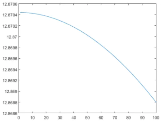
In this subsection we fix p = 0.5 and calculate the option’s value as we change x, i.e., ast(1) andt(2) become more distant fromt = 0.5.
3.1.2 Fixed moments when dividends are paid
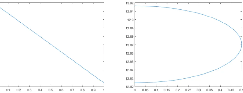
In this subsection, we break the randomness symmetry by varying p and introducing skewness in the distribution about the moment when dividends are paid. For (t(1), t(2)) = (0.4,0.6) we get the following graphs
Figure 2: Value of the option as a function of (a) the probability p and
(b) standard deviation of the random time when dividend is paid
p
p(1−p) (M=10000,Nat=5)
Figure 2a shows that the value of the option decreases linearly as p increases. Figure 2b shows that changes in the value of the option are more sensitive whenever there is more uncertainty about the moment when dividends are paid.
3.1.3 Varying probability and moments when dividends are paid
In this subsection we vary simultaneously p∈[ 0,1] andx∈[ 0,1/2] .
Figure 3: Values for differentp as a function of x
Figure 3 describes the value of the option for different values of x. The upper line is for p= 0.01 and the lower line is for p= 1. Each of the lines correspond to a different value of p, and two different lines never intercept each other. These lines appear to be linear due to the scale used. In fact none is linear, although they get closer to linear, as x increases.
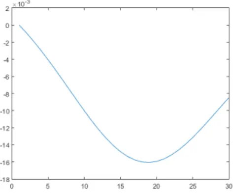
By adjusting the vertical scale in Figure 4 we better see how increasing concave curves become decreasing as p increases.
Figure 4: Concave values as a function of xfor: p= 0.493, p= 0.495, p= 0.497, p= 0.498 (M=10000,Nat=5)
There is no value ofpdifferent from 0 or 1 that makes the value function linear, implying that concavity reflects the uncertainty abut the time at which dividends are paid.
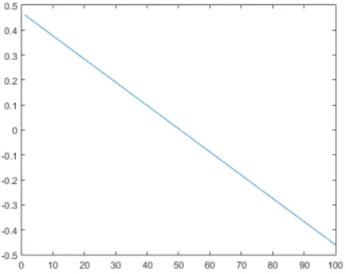
We next examine the derivative of the value function at x = 0. This follows from the expression of V, since
dV
dx|x=0 =−pV
′+ (1−p)V′ = (1−2p)V′
. The only situation where a null derivative atx= 0 happens is when p= 0.5. Forp > 0.5 this derivative is negative, and forp <0.5 is positive. This is illustrated in Figure 5 below obtained numerically (M=1000000,Nat=12).
Figure 5: Derivative of the option value at x= 0 as function of p Notice that the slope of this straight line is −2V′ and its value is only 0
the value of this slope is the central element to understand how sensitive the value of the option is to the uncertainty regarding the moment when dividends are paid. In what follows we shall refer to this variable as the slope.
3.2
Sensitivity analysis
In this section we analyse how our results depend on the parameters of the stochastic process driving the value of the underlying asset. The original parameters of our analysis were: S= 110;r = 0.03, σ= 0.2, K = 100, D = 5, T = 1, x. The parameters are classified in two categories: the first related with the time value of the option (r, σ, T, x); the second are fixed contractual values (S, D, K).
3.2.1 First class of parameters
Let us first consider the no-dividend case in the Black-Scholes context. A change inT can be trivially compensated by a simultaneous change inσand r such thatrT and σ2T remain invariant. This result reflects a property of the geometric Brownian motion implying the following: given two points in time τ1 and τ2, the probability that the value of the underlying asset is in an arbitrary interval atτ1 is the same as attaining that same interval at τ2, provided the volatility and interest rate are suitably adjusted.
Following this reasoning, in the case where the underlying asset pays a dividend at eitherT /2−xorT /2+x, a change inT will not affect the value of the option provided that not only σ and r are adjusted as above, but also x/T remains invariant. An increase in T will postpone proportionally the dates where the dividends may be paid, but the adjustments in σ and r will guarantee that the probabilities remain invariant.
For example with T = 1 and S = 110, r= 0.03, σ = 0.2, K = 100, D = 5, x = 0.1, a change to T = 3 would imply a change in the parameters to S = 110, r = 0.01, σ = 0.2q13 ≈ 0.11547, K = 100, D = 5, x = 0.3, in order to preserve the value of the option.
Since changes in T can be assimilated by changes in r, σ and x, we proceed with the sensitivity analysis keeping T constant.
Going back to the final remark after Figure 5, the only interesting fea-ture that characterizes by how much the value of the option increases or decreases around x = 0 is the slope of that graph, characterized by V′.
Therefore, as we change the parameters in our model only the slope of the graph will change, the straight line rotating around the point where p= 0.5.
Let us maintainσ = 0 when analysing how varyingr impacts the slope. In Figure 6 below we can see how the slope of the first order derivative graph behaves with several values of r. In the horizontal axis we have r=−0.1 (1) untilr= 0.1 (40), in equal increases of 0.005 per interval.
Figure 6: Slope of the derivative at x= 0 as a function of r (M=10000,Nat=5)
Asr >0, the slope of the first order derivative graph becomes more negative as r increases.
For r < 0 small enough, the slope is positive - this is the region where r is negative but the value of the option is positive. The positive slope reflects an aspect of the negative time value of money, as discussed in the conclusions.
If we keep decreasing r beyond that interval, the value of the slope will jump to 0 and will stay flat at that level. This happens because the underlying asset does not fluctuate (since σ = 0), only being discounted in time at the negative rate r. It thus follows that for an option to have a positive value under a negative enoughr, it is necessary that σ >0.
Figure 7: Slope of the derivative at x= 0 as a function of σ (M=10000,Nat=5)
In the horizontal axis of Figure 7 the values of σ range from 0(1) to 0.78(40), in equal intervals of size 0.02 (since σ is always positive). The slope results as a decreasing function ofσ. It follows that the higherσ the better it is for the dividend to be paid at t(2).
In what follows we focus on the impact of r and σ on the value of the option when the values of these parameters are both different from 0.
Figure 8: Slope of the derivative at x=0 as a function of σ for several values of r (each line represents one r)(M=10000,Nat=5)
In Figure 8 we observe the behaviour of the slope for simultaneous variations on r and σ. Each line represents how the slope decreases as the value of σ increases, for a fixed value of r. The top and bottom lines corresponds respectively to r = −0.02 and r = 0.07. In the horizontal axis, there is a scale of 1 to 10, where 1 representsσ = 0 and 10 represents σ = 0.36, in equal increases of 0.04. A positive slope can be attained for negative r and a sufficiently lowσ.
slope will be given by
d(sl) = ∂sl ∂rdr+
∂sl ∂σdσ,
knowing that both partial derivatives are negative. The resulting increment in the slope may thus be either positive or negative, depending on the relative variation in both r and σ.
Since this section is characterizing the slope of the option value atx= 0, we now turn to a corollary of the slope construction: the value of the option is more sensitive to the value ofp, the larger the absolute value of the slope. This result has two interesting implications. First, as shown in Figure 9 below, a simultaneous increase inr and σ requires a larger range of change in p in order to make the option value a monotonic (increasing) function of x. This makes explicit the higher sensitivity of the option value on the skewness of the uncertainty as expressed by p.
Figure 9: Pictures above replicate initial parameters from section 3.1: p= 0.493, p= 0.495, p= 0.497, p= 0.498.
The graphs in the bottom line are obtained with new parameters: p= 0.482, p= 0.484, p= 0.488, p= 0.492 with r= 0.1 andσ = 0.5.
(M=10000,Nat=5)
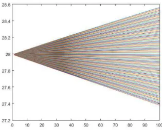
Figure 10: Values for differentp as a function of x
2 (M=400,Nat=2) The larger the absolute value of the slope, the wider this cone is. This implies that for any given x, the larger the slope, the larger will be the impact of the skewness (as reflected by p) in the value of the option.
We finish the analysis on this class of parameters going back to T. We know that a change in T must be compensated by a simultaneous change in σ and r such that rT and σ2T remain invariant. This implies that an increase in T (and proportionally in x) will decrease the absolute value of the slope (i.e. it will become a smaller negative slope).
3.2.2 Second class of parameters
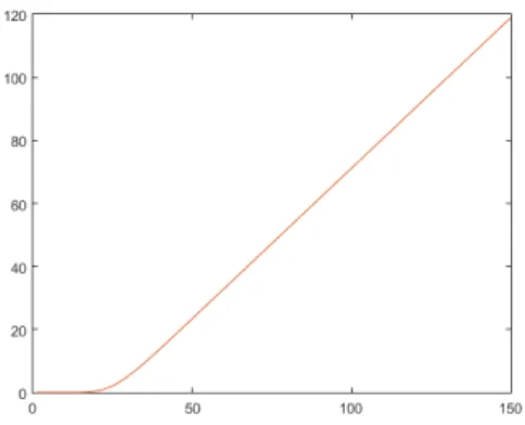
Figure 11: Value for the call option as a function of λ(M=400,Nat=2) From the exposed above, the value of the option is preserved, provided all three parameters are suitably linearly adjusted. We now focus on the impact of not adjusting the exercise price K. This affects the probability that the option is exercised at maturity. Figure 12 below illustrates this point, replicating Figure 11 but keeping K = 30 fixed. Here the graph is non-linear, approaching linearity asymptotically as S increases.
Figure 12: Value for the call option as a function of λ whenK is not adjusted (M=400,Nat=2)
Non-linearity results follows from the fact that the option value is an homogeneous function of first degree in the three parameters. By not ad-justing one of them, non-linearity clearly results.
In fact, by not adjusting K the probability of exercising the option increases for λ >1 and decreases for λ <1.
finish out of the money. For every such sample path, a slightly lower initial value of the underlying asset would also end out of the money. However for some of the paths starting atS0 and ending in-the-money, a decrease in the initial value of the underlying asset may lead to an out of the money result. Thus decreasing S0 results in less sample paths that end in-the-money (re-ducing the probability that the option is exercised). The difference to the case where dividends are paid is simply that the probability of ending out of the money is larger than in the no-dividend case. As the value of the option is the expected payoff calculated as the weighted average over all the sample paths, the basic properties of monotonicity and convexity as a function of the initial value of the underlying asset are not changed.
We decompose the relation between S, K and D in the study of the ratios S/K and S/D. We will analyse the behaviour of S/D by varying D and keeping S and K constant. We will then vary K and analyse the behaviour ofS/K while keeping S and D constant.
Starting with S/D we vary D between 0 and 30 so that the ratio D/S lies between 0 and 30/110. We present in Figure 13 the graph for the slopes of the first order derivative graphs (r = 0, σ = 0.2):
Figure 13: Slope of the derivative at x=0 as a function of D (M=10000,Nat=5)
Clearly the slope is always negative. At D = 0 the slope is naturally 0 since in the absence of dividends the probability p plays no role. As D increases the slope decreases (becomes increasingly negative) since the impact of pin the option value increases. This is true until a certain point D+, where the impact of p starts reverting.
For sufficiently large value of D, the advantage of paying the dividend att(2) instead oft(1) becomes smaller since there is a greater chance that the option will be worthless at maturity. This explains the behaviour of the graph fromD+ onwards.
advantage of a later payment at t(2). The graph in Figure 13 shows that at D+ the trade-off between these effects is marginally dominated by the probability of ending out of the money. Notice that the effect is never completely offset as the slope increases but never reaches 0 (there is always a positive probability of ending in the money). With the parameters used in this study we find D+≈18.
Figure 14 below has a positive r = 0.03, and a smaller , σ = 0.1 for us to perceive better the effects mentioned above. The values of D ranges from 0 to 58 in the horizontal-axis.
Figure 14: Slope of the derivative at x=0 as a function of D(M=10000,Nat=5)
Figure 15 is similar to Figure 14 (including the scale of the horizontal axis) but using σ = 0.2 instead of σ= 0.1. It takes longer for the slope to start increasing as D increases. D+ ≈ 30 (Figure 15) > D+ ≈ 20 (Figure 14). As we recall, the increase inσ always decreases the value of the slope.
Figure 15: Slope of the derivative at x=0 as a function of D(M=10000,Nat=5)
4 and Figure 10 but increasing the value of the dividend to: D= 18 (left) and D = 40 (right). As expected, the cone is farther away with a higher negative slope.
Figure 16: Values for differentp as a function of x
2 (D=18 on the left) (D=40 on the right)(M=10000,Nat=5)
Figure 17, below on the left, presents the values of the slope (vertical axis) for 10 different values ofD, ranging from 0 to 36 (horizontal axis) in equal increments of 4. Each line has one value r from -0.02 (top line) to 0.07 (bottom line). σ= 0.2.
With the increase in r the value for D+ increases slightly. There is not any positive value for the slope in the graph, as with σ = 0.2 only with a very high negative interest rate the slope would be positive as shown in Figure 8. Figure 17, using the same scale for r, would have had positive values for a small enough σ. In the conclusions about negative interest rates we will study that example.
In Figure 17, below on the right, we have again the values of the slope in function ofD. The scale for the horizontal-axis is the same butr is fixed at 0.03 and each line has σ varying between 0 and 0.36.
For σ = 0, from a dividend value slightly over D = 13 the slope is 0 as the option becomes worthless. For other values of σ it never reaches 0 (there is always a chance thatST > K). The remaining of Figure 17 shows
Figure 17: Slope of the derivative at x= 0 as a function of D for σ fixed and several values of r (left) and for r fixed and several values for σ
(right) (M=1000,Nat=5)
In the next figure below we change the ratioS/K. Figure 18 represents the slope for a change in K from 0 to 245 in increments of 5.
When K is equal or close to 0, the chance that the option will end up below K is small, which makes the slope to be close to the value of
−r, because a change in p originates the value of the option to change
≈ −ret(2)−t(1) ≈ −re0 = −r. For K = 0 the value of the slope is there-fore exactly −r. When we increase K, the chance that the value of the underlying asset ends up below K increases, resulting in a decrease slope. However, from a certain K onwards, which we will call K+ the value of the slope will increase remaining negative, never reaching 0 (it will still be better for the value of the option that the dividend is paid at t(2)). Using this parameters it is K+ ≈108.
The advantage by paying at t(2) versus t(1) (because of the time value of money), will start to be offset by the effect that a higherK increases the probability that the option will not be exercised ( if not exercised results on no difference betweent=t(1) or t=t(2)). It is a similar logic that was used to explain D+ above in this subsection.
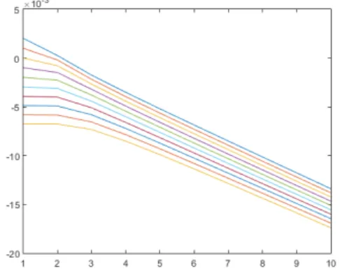
Figure 19 below presents the change in the slope when we vary D for 10 different lines where each one represents a different value forK (from 0 to 180, in increases of 20). Figure 19 , on the left, has a scale in horizontal axis of D from 0 to 27, and Figure 19 ,on the right, of D from 0 to 45. For all the values of K the graph is convex but as K increases D+ gets smaller. For example the blue line has a higher K than the green line. The reasoning behind it is that with a higher K, for the same value D, the probability that the option will be worthless is higher. Therefore, with a higher K, marginally offsetting the time value of money effect from a smaller D+ onwards.
Figure 19: Slope of the derivative at x= 0 as a function of D. Each line represent one value for K. (M=1000,Nat=5)
Figure 20: Slope of the derivative at x= 0 as a function of K. Each line represent one value for r (M=10000,Nat=5)
In the below Figure 21 we have 10 lines for each value of σ, ranging from 0 to 0.36. We setr constant to 0.03,K ranging from 20 to 180. Asσ becomes smaller the graph also shrinks. As expected it has a slope value equal to −r for K = 0 for any value of σ. The way the value for the slope behaves in Figure 21 is somewhat similar to Figure 20, as expected from previous analysis.
Figure 21: Slope of the derivative at x= 0 as a function of K. Each line represent one value for σ (M=10000,Nat=5)
4
Analysis of results
4.1
Impact of uncertainty skewness
Our first main conclusion is that for standard values of the model’s pa-rameters, the main factor that affects the option value under uncertain dividend date is the skewness of the payment date distribution. For an even distribution the vale of the option decreases as compared with the case of a deterministic date; for positive skewness (expected anticipation of the ex-dividend date) the value of the option also decreases, whereas for negative skewness (expected delay of the ex-dividend date) it increases this value.
The basic argument for this result reflects time value of money (positive interest rates) in the sense that a later dividend have lower present value than an earlier dividend. So, if for a dividend paid at a certain date the option has a certain value, expecting the dividend to be paid later (all other parameters equal) will tend to increase the value of the option. Likewise, expecting dividend to be paid earlier will lower the value of the option.
In our analysis we evaluated how sensitive the value of the option was for possible dividend dates very close to the deterministic date. The sensitivity was measured by the derivative of the value function as a function of that difference in dates, when that difference is very small. We next studied the behaviour of that derivative with respect to skewness as measured by the probabilistic parameter p. This introduced what we called the slope: the derivative may decrease withp(negative slope) or increase withp(positive slope).
It is worth mentioning again that a negative slope implies the conclusion that it is better to delay the dividend, whereas a positive value for the slope implies that it is better to anticipate the dividend. The absolute value of the slope is important to understand how relevant i.e. how sensitive the value of the option is to changes in p.
However, if interest rates are negative, volatility is small enough and the option is sufficiently in the money, the impact of skewness on the value of the option is reverted. In the next subsection we analyse the impact of negative interest rates.
4.2
Impact of negative interest rates
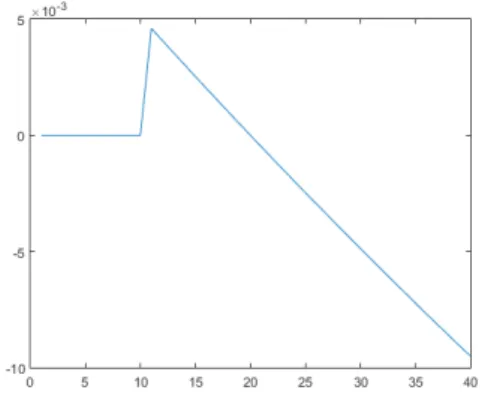
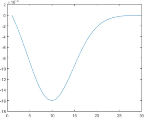
Figure 22: Slope of the derivative at x= 0 as a function of D. (M=10000,Nat=5)
The top part of Figure 22 shows the slope as D increases and r =
−0.03 with σ = 0.05. There is an initial interval that presents a positive slope. This means that in that region anticipation of the dividend payment increases the value of the option, reflecting the fact that the time value of money is negative. However, an increase in the value of the divided to be paid reverts this result: delaying the dividend increases the value of the option, reflecting that other factors dominate the time value of money effect.
This means that above a certain critical value of the dividend, the impact on the probability of ending in the money dominates the time value of money of the dividend, making it preferably to delay the payment of dividends in spite of the negative interest rates.
The remaining graphs in Figure 22 present the same effect for a shorter range of dividend values (from 0 to 7) with σ = 0. The left graph is for r = −0.03 and the right one for r = −0.02. Without volatility, the values for the option are positive until SerT
Figure 23: Slope of the derivative at x=0 as a function of σ for several values of r (each line represents one r) K=100 (M=10000,Nat=5) Additionally the positive value of the slope in Figure 22 is only possible if σ is sufficiently small. The graph in Fgure 23 shows decreasing lines for the value of the slope as a function of volatility. Each line represents a different value of r. The upper line is for r = −0.02 and the lower line is forr = 0.07. For anyσ > 0 , it is possible to find a negative enoughr such that the slope is positive.
It is clear from this graph that the parameter that strongly impacts the probability of ending in the money, thus dominating the time value of money effect when interest rates are negative, is the volatility of the underlying asset.
The critical value of σ below which the slope for negative interest rate becomes positive depends on the value of the ratio S/K, or the in-the-moneyness of the option. Deep in the money options require an extremely high σ for a negative slope.
Above a critical value ofK, the value of the slope will never be positive for any combination ofrandσ. This critical value isK =SerT
Figure 24: Slope of the derivative at x=0 as a function of σ for several values of r (each line represents one r). The graphs are per order with K
equal to: 103, 108, 110, 113 , 140 (M=10000,Nat=5)
Figure 24 illustrate similar graphs to the one in Figure 23, but for different values of K above the original parameter K = 100, corroborating our previous statement: only in the first graph (for K = 103) it is possible to get a positive slope; for higher values of K the slope is always negative for the parameters used.
We thus conclude that if interest rates are negative, the time value of money effect dominates, provided that volatility is sufficiently small and the option is sufficiently in the money.
4.3
Implications for hedging
We may also discuss the implications for hedging of the option. Beyond the natural uncertainty about the value of the underlying asset, there is an additional uncertainty about the time when dividends are paid. This additional uncertainty implies accrued risk to the payoff of the option.
As
V =pV(0.5−x) + (1−p)V(0.5 +x)
the option with uncertain dividend date can be replicate by a weighted combination of two options: one that pays early dividends att(1) = 0.5−x and another one that pays later dividend at t(2) = 0.5 +x.
All the greeks for this option are clearly the weighted averaged greeks for the two options that compose the replicating portfolio.
5
Conclusions
In this paper we have analysed the impact of uncertain dividend payment dates in the value of a European option.
the section that analyses the results. The basic ingredient is the trade-off between the dividends’ present value and the probability of ending in-the-money in the cases where dividends might be slightly anticipated or delayed. When interest are negative the present value effect reverts and the trade-off depends on the in-the-moneyness of the option and the volatility level of the underlying asset.
The analysis was conducted under a simple bimodal distribution for the dividend dates, but the main conclusions seem to be extendible with-out loss of generality. It would be of interest to understand the possible impact of higher moments (kurtosis) of such distributions in the value of such European options. For that purpose a more sophisticated model of uncertainty would be required.
References
[1] Beneder, R. and Vorst, T. (2001) ”Option on dividend paying stocks”, Recent Developments in Mathematical Finance, in Proceedings of the International Conference on Mathematical Finance, Shanghai, China, World Scientific, Singapore.
[2] Black, F. (1975) ”Fact and fantasy in the use of options”, Financial Analysts Journal, Vol.31, July-August, pp. 36-41, 61-72.
[3] Black, F. and Scholes, M. (1973) ”The pricing of options and corporate liabilities”, Journal of Political Economy Vol.81, pp. 637-59 .
[4] Amaro de Matos, J., Dil˜ao. R. and Ferreira, B. (2009) ”On the value of European options on a stock paying a discrete dividend”, Journal of Modelling in Management Vol.4, pp. 235-248 .