3D Lung Nodule Classification in Computed Tomography Images

F

E

U

P

3D Lung Nodule Classification in

Computed Tomography Images

Ana Rita Felgueiras Carvalho

Mestrado Integrado em Engenharia Electrotécnica e de Computadores Supervisor: Aurélio Joaquim de Castro Campilho

Supervisor: António Manuel Cunha

c

3D Lung Nodule Classification in Computed Tomography

Images

Ana Rita Felgueiras Carvalho

Mestrado Integrado em Engenharia Electrotécnica e de Computadores

Resumo

O cancro do pulmão é a maior causa de morte por cancro em todo o mundo. O diagnóstico é muitas vezes realizado pela leitura de tomografias computadorizadas, TC’s - uma tarefa propensa a erros. Existe bastante subjetividade na avaliação do diagnóstico do nódulo. Esta, entre outras causas, podem levar a um diagnóstico inicial incorrecto o que pode ter um grande impacto na vida do paciente [1]. O uso do sistema Diagnóstico Assistido por Computador, CADx, pode ser uma ajuda para este problema, fornecendo uma segunda opinião aos médicos quanto ao diagnóstico da malignidade dos nódulos pulmonares. No entanto, os médicos acabam por evitar o uso destes sistemas [2], pois não conseguem perceber o “como e porquê” dos resultados que apresentam. De forma a aumentar a confiança dos médicos nos sistemas CADx, Shen et al. [3] propuseram uma rede neuronal convolucional semântica hierárquica profunda, HSCNN, que para além de ter como resultado um diagnóstico de malignidade, prevê também características semânticas rela-cionadas com o mesmo, demonstrando assim evidências visuais do diagnóstico. Como entrada para a HSCNN, Shen et al. usaram a LIDC-IDRI, Lung Image Database Consortium and Image Database Resource Initiative, uma base de dados pública que contém 2,668 nódulos anotados por radiologistas relativamente a algumas das características semânticas que apresentam [4].

Esta base de dados contém bastante variação entre as avaliações dadas pelos médicos, para o mesmo nódulo, na mesma característica, principalmente nas características lobulação e espicu-lação, as duas da base de dados com mais relevância para a malignidade. Por essa razão, Shen et al. não previram na sua rede essas duas características. Motivada por estas razões, uma questão sugerida por Shen et al. foi levantada: com a diminuição da variabilidade nas avaliações das características semânticas, será que a previsão da malignidade na HSCNN irá melhorar?

Para responder a esta pergunta foi apresentada como uma possível solução a obtenção de de um dataset LIDC-IDRI anotado de forma mais coerente. Para tal, foi realizada inicialmente uma análise à base de dados e uma revisão da literatura, que permitiu a criação de critérios de avaliação das características semânticas mais exatos do que os existentes. Depois destes serem criados e validados por radiologistas do Centro Hospitalar do São João, foi reanoatada a base de dados LIDC-IDRI, seguindo uma metodologia proposta com base nos critérios concebidos. Finalmente, a base de dados reclassificada foi usada como entrada para a rede HSCNN, de forma a avaliar o impacto que esta tinha na previsão da malignidade. Foram utilizados 1,386 nódulos e todas as anotações foram binarizadas. O treino da rede foi realizado usando 4-fold cross-validation.

Os resultados desta solução proposta apenas foram melhores, comparativamente ao trabalho de Shen et al., nos valores de sensibilidade, existindo uma melhor previsão de quando os nódulos são realmente malignos. A previsão da malignidade teve uma exatidão de 0.78, uma área sob a curva da característica de operação do receptor, AUC da ROC, de 0.74, uma sensibilidade de 0.83, e uma especificidade de 0.89. No trabalho de Shen et al. foram obtidas uma exatidão de 0.84, uma AUC da ROC de 0.86, uma sensibilidade de 0.71 e uma especificidade de 0.89. Uma análise às previsões incorretas revelou que a maior parte destas eram compostas por nódulos pequenos, com bastante matéria à volta, com calcificação sólida ou juxta-pleurais. Os nódulos corretamente

ii

previstos eram na sua maior parte solitários, ou com tecido de pleura adjacente. No entanto, esta comparação com o trabalho de Shen et al. não é linear, pois o número de dados usado foi diferente (1,386 nódulos foram usados neste trabalho ao invés de 4,252 no trabalho de Shen et al.) e a conversão das avaliações para binário foi também realizada de outra forma, o que pode ter tido influência nos resultados finais.

Com base nos resultados obtidos ao utilizar a metodologia proposta para a diminuição da variabilidade nas avaliações das características semânticas da LIDC-IDRI, foi verificado que não existe uma melhoria na previsão do diagnóstico da malignidade na HSCNN, comparativamente aos resultados de Shen et al..

Abstract

Lung cancer is the leading cause of cancer death worldwide. Usually, the diagnosis is made by physicians reading computed tomographies, CTs - a task prone to errors. There is a lot of sub-jectivity in the nodules’ diagnose assessment. That, among other causes, can lead to an incorrect initial diagnosis, delaying the correct treatment, which can have a high impact on the patient’s life [1]. The use of Computer-Aided Diagnosis, CADx, can be a great help for this problem by assisting doctors assessing lung nodule malignancy, giving a second opinion. However, physi-cians end up avoiding the use of CADx [2], because can not understand the “how and why” of its diagnostic results. To increase the physicians’ confidence in the CADx system, Shen et al. [3] proposed a deep hierarchical semantic convolutional neural network, HSCNN, that besides hav-ing as result the malignancy’ diagnosis, also predicts the features related to it, givhav-ing this way visual evidence of the diagnosis. As input for HSCNN Shen et al. used LIDC-IDRI, Lung Image Database Consortium and Image Database Resource Initiative, a widely used public dataset, that has 2,668 abnormalities annotated by radiologists regarding the semantic features that they present [4].

This dataset has a high variance between the assessments given by physicians, for the same nodule, in the same semantic feature, especially in lobulation and spiculation, the two LIDC-IDRI features most relevant to malignancy. For this reason, Shen et al. did not predict in their work these two characteristics. With that motivation, a question suggested by Shen et al. was raised: will the decrease of variability in LIDC-IDRI semantic features evaluations improve the HSCNN malignancy prediction?

To answer this question was presented as a possible solution to obtain a more coherently annotated LIDC-IDRI dataset. For this purpose, a dataset analysis and literature review were initially realised, which allowed the creation of more accurate semantic characteristics evaluation criteria than the existing ones. After these were created and validated by radiologists at the São João Hospital Center, the LIDC-IDRI database was revised, following a proposed methodology based on the devised criteria. Finally, the reclassified dataset was used as input to the HSCNN to evaluate its impact on malignancy prediction. 1,386 nodules were used and all annotations were binarised. The network training was performed using 4-fold cross-validation.

The results of this proposed solution improved only, compared to the work of Shen et al., in the sensitivity, with a better prediction of when the nodules are truly malignant. The malignancy prediction obtained an accuracy of 0.78, an area under the receiver operating characteristic curve, AUC of ROC, of 0.74, a sensitivity of 0.83, and a specificity of 0.89. In the Shen et al. work were obtained as accuracy 0.84, as AUC of ROC 0.86, as sensitivity 0.71 and as specificity 0.89. The analysis of the network incorrect predictions revealed that most of them were small nodules, with a lot of matter around, with solid calcification, or juxta-pleural. The correctly predicted nodules were solitary, or with pleural-tail. However, the comparison with Shen et al. work is not linear since the quantity of data used was different (1,386 nodules instead of the 4,252 used in Shen et al.work) and the conversion to binary was also performed differently, which may have influenced

iv

the final results.

Based on the results obtained, using the proposed methodology to the decrease of LIDC-IDRI semantic features evaluations variability, it is verified that there was no increase in malignancy prediction in HSCNN, comparing to Shen et al. results.

Acknowledgments

Ao co-orientador António Cunha, pela constante preocupação e orientação na duração desta dis-sertação e por me ter proporcionado a oportunidade de trabalhar nesta área. Ao grupo C-BER, pela sua companhia e ajuda.

Ao Diogo Moreira, e Daniela Afonso por me terem acompanhado fielmente nestes últimos 6 anos, por termos crescido tanto juntos. À Mariana Caixeiro, por toda a amizade e conversas em que as palavras não são necessárias.

À Manuela Rodrigues e Sara Alves, por me fazerem acreditar que existem amizades que po-dem durar para sempre. Por serem uma parte da minha alma, por me darem um pouco da sua força, e acreditarem em mim sempre, mesmo quando eu não acreditei. Nunca vão existir palavras suficientes. À Daniela Afonso, mais uma vez, por me mostrar o que é a amizade na sua mais pura forma de ser. Por me ter acompanhado nas fases mais, e menos, belas da minha vida, e por sempre nos termos compreendido na essência do que somos. Obrigada às três por, conhecendo todas as minhas versões, me ajudarem sempre a ser a melhor.

Ao Diogo Pernes, por toda a paciência, apoio e companhia, imprescindíveis nesta etapa da minha vida. Por tudo o que me ensinou e por ter tornado isto possível. Obrigada por presenteares os meus dias com o teu brilho.

À minha família, a quem devo grande parte do que sou. Ao meu Pai, por me dar o privilégio de sentir tudo. Ao meu Irmão, Miguel, por trazer tanto amor no seu coração e transborda-lo para o meu. À minha Mãe, por representar a beleza mais pura do meu mundo. À minha Avó Lina, por me ensinar que o amor é o maior ensinamento da vida.

Ana Rita Felgueiras Carvalho

“Procura em ti O que não encontrares Em lado nenhum”

Mariano Alejandro Ribeiro

“É naquilo que faço que encontro o que procuro”

Contents

2.2 Lung Cancer Diagnose . . . 7

2.3 Computer-Aided Diagnosis System . . . 10

2.4 Summary . . . 10

3 Literature Review 11 3.1 Deep Learning Fundamentals . . . 11

3.1.1 Neural Networks . . . 12

3.1.2 Convolutional Neural Networks . . . 16

3.1.3 Learning . . . 18

3.2 LIDC-IDRI Dataset . . . 21

3.3 Lung Nodule Classification Methods . . . 23

3.4 Discussion . . . 28

3.5 Summary . . . 30

4 Methodology 31 4.1 LIDC-IDRI Analysis . . . 32

4.1.1 Dataset Review Tool . . . 32

4.1.2 LIDC-IDRI Semantic Features Bibliographic Review . . . 34

4.2 Dataset Reassessment . . . 42

4.3 Impact Evaluation . . . 44

4.4 Summary . . . 47

5 Results and Discussion 49 5.1 Evaluation Norms . . . 49 5.2 Dataset Reassessment . . . 54 5.3 Impact Evaluation . . . 57 5.3.1 Dataset Preparation . . . 57 5.3.2 Training . . . 60 5.3.3 Results . . . 61 5.3.4 Discussion . . . 65 ix

x CONTENTS

5.4 Summary . . . 70

6 Conclusions and Future Work 71

A Worksheet File 73

B Norms 77

List of Figures

1.1 Age Standardized incidence Rates vs. Mortality Rates, in 2018 [5]. . . 1

2.1 Lungs anatomy and structure [6]. . . 6

2.2 Original CT slice with lung tissues localization and intensity values are given in HU [7]. . . 7

2.3 Characterization by nodule’s location from [8]. . . 8

2.4 Characterization by nodule’s intensity from [8]. . . 8

2.5 Lung nodules from [4], representing solid, non-solid, and part-solid densities, in axial view. . . 9

3.1 Artificial neuron. . . 12

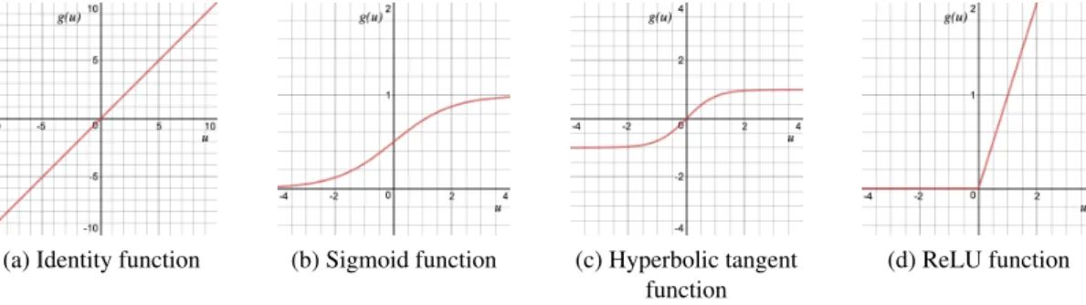
3.2 Identity, logistic sigmoid, hyperbolic tangent and ReLu functions graphics. . . . 14

3.3 Multilayer perceptron, with one hidden layer. . . 14

3.4 Comparison between a typical MLP and a CNN, the red input layer holds the image, so its width and height would be the dimensions of the image, and the depth would be 3 (red, green, blue) channels.) [9]. . . 16

3.5 Example of a convolution operation, with two filters of size 3x3, applied with a stride (the length that the kernel is moving) of 2 [9]. . . 17

3.6 Max pooling layer operation with kernel size 2x2 and stride length 2. . . 18

3.7 CNN example, with an output of 5 classes [9]. . . 18

3.8 Multi-crop architecture [10]. The numbers along each side of the cuboid indicate the dimensions of the feature maps. . . 23

3.9 Multi-crop pooling [10]. . . 24

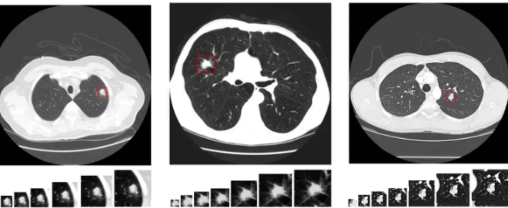
3.10 CT examples of the three types of ternary classification (from left to right, benign, primary malignant and metastatic malignant) with, in each one, the different 7 different views areas, from left to right 20x20, 30x30, 40x40, 50x50, 60x60, 70x70 and 80x80, taken from [11]. . . 25

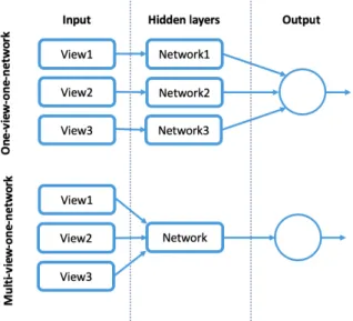
3.11 Multi-view’s strategies: one-view-one-network(top) and multi-view-one-network (bottom). . . 26

3.12 The architecture of3.12awas taken from [11] and architectures from figures3.12b

and3.12cwere taken from [12]. . . 26

3.13 HSCNN architecture taken from [3]. . . 27

4.1 The methodology used for LIDC-IDRI review and impact evaluation in the malig-nancy prediction. . . 31

4.2 Nodule images from [4], without and with binary mask in axial, coronal, and sagittal planes. . . 33

4.3 Popcorn, laminated, solid, non-central, central and absent calcification example nodules from LIDC-IDRI dataset [4]. . . 36

xii LIST OF FIGURES

4.4 Malign and benign types of calcification by [13]. . . 37

4.5 Internal structure’s examples. 4.5ais from LIDC-IDRI dataset [4], and4.5band 4.5care from [14]. . . 38

4.6 Non lobulated and lobulated nodules examples from LIDC-IDRI dataset [4]. . . . 38

4.7 Poorly defined and sharp margins nodules from LIDC-IDRI dataset [4]. . . 39

4.8 Linear and round nodules examples from LIDC-IDRI dataset [4]. . . 40

4.9 No spiculated and spiculated nodules examples from LIDC-IDRI dataset [4]. . . 41

4.10 Extremely subtle and obvious nodules examples from LIDC-IDRI dataset [4]. . . 42

4.11 Method used to do the dataset reassessment. . . 43

5.1 Nodule with a non-central calcification that has an LIDC-IDRI’s doctors averages evaluation of central calcification from [4]. . . 50

5.2 Implemented 4 fold cross-validation. . . 61

5.3 Confusion matrices for each semantic feature, using fold 2 as test set. . . 63

5.4 ROC curve for each semantic feature, using fold 2 as test set. . . 64

5.5 Malignancy ROC curve for fold 2, with an AUC = 0.74. . . 65

5.6 Nodules images with their predictions and truth labels. . . 66

A.1 Nodule information, and evaluations’ average given by the doctors, in the work-sheet file. . . 73

A.2 Classifications given by a doctor in evaluation 1, in the worksheet file. . . 74

A.3 Nodule’s images without and with the average binary mask of the doctors, in the worksheet file. . . 75

B.1 Calcification and its classes definition. . . 77

B.2 Very small nodules for each class in calcification. . . 77

B.3 Small and big nodules for each class in calcification. . . 78

B.4 Lobulation and its classes definition. . . 78

B.5 Very small for each class in lobulation. . . 78

B.6 Small and big nodules for each class in lobulation. . . 79

B.7 Margin and its classes definition. . . 79

B.8 Very small for each class in margin. . . 79

B.9 Small and big nodules for each class in margin. . . 80

B.10 Spiculation and its classes definition. . . 80

B.11 Very small for each class in spiculation. . . 80

B.12 Small and big nodules for each class in spiculation. . . 81

B.13 Subtlety and its classes definition. . . 81

B.14 Very small for each class in subtlety. . . 81

B.15 Small and big nodules for each class in subtlety. . . 82

B.16 Texture and its classes definition. . . 82

B.17 Very small for each class in texture. . . 82

List of Tables

3.1 Explanation of various cases with results of Disease vs Test. . . 20

3.2 LIDC nodule characteristics, definitions and ratings proposed in [15]. . . 22

3.3 Binary labels proposed by Shen et al. [3] from LIDC-IDRI rating scales for nodule characteristics. . . 28

3.4 Results comparison between 3D CNN and HSCNN. . . 29

3.5 Results for semantic features predictions . . . 29

3.6 Final best results for the different relevant CNN’s architectures presented . . . . 30

4.1 Characteristics and their classes in LIDC-IDRI dataset proposed by Opulencia et al.[15] . . . 35

5.1 Ratings division obtained from the analysis. . . 53

5.2 Comparison between the nodules number in the original and reclassified datasets 56 5.3 Characteristics conversion from ternary to binary classification. . . 58

5.4 Ratings division obtained from the binarisation. . . 58

5.5 Total number of nodules for each characteristic . . . 59

5.6 Total number of nodules for each characteristic and malignancy, after selecting only the abnormalities that had 3 or more evaluations in LIDC-IDRI . . . 60

5.7 Average test results for each semantic feature. . . 62

5.8 Best test results for each semantic feature, using fold 2. . . 62

5.9 Test results for each fold, for lung nodule malignancy prediction. . . 62

5.10 Confusion matrix for malignancy, using fold 2 as test set . . . 63

Abbreviations and Symbols

3D Three Dimensional

2.5D Two-and-a-half Dimensional ANN Artificial Neural Network AUC Area Under the Curve CADx Computer-Aided Diagnosis CNN Convolutional Neural Network CT Computed Tomography GGO Ground Glass Opacity

HSCNN Hierarchical Semantic Convolution Neural Network IRB Institutional Review Board

k-NN K-Nearest Neighbors

LDCT Low Dose Computed Tomography

LIDC-IDRI Lung Image Database Consortium image collection LNDetector Lung Detector

MLP Multilayer Perceptron

MRI Magnetic Resonance Imaging

MVCNN Multi-view Convolutional Neural Network MC-CNN Multi-croop Convolutional Neural Network ReLU Rectified Linear Unit

ROC Receiver Operating Characteristic SGD Stochastic Gradient Descent SVM Support-Vector Machine

Chapter 1

Introduction

Lung cancer is the pathology that has more mortality globally, accounting for more deaths than cancers of the breast, prostate, colon, and pancreas combined [16]. Worldwide, it was estimated to be the cause of death of 1,761,007 people, from both sexes, on a total of 2,093,876 incidences (giving a death rate of 84%, when is known to have cancer), in 2018 [5].

In Portugal, the International Agency for Research on Cancer [17] estimated that in 2018 one-quarter of the population is in risk of developing cancer until 75 years, expecting 5,284 incidences, having a standardized rate per 100,000 of 22.6%, from both sexes, and all ages. To a better per-ception of the problem, the incidence and mortality age-standardized rate per 100,000 population, for other world areas could be seen in Figure1.1.

Figure 1.1: Age Standardized incidence Rates vs. Mortality Rates, in 2018 [5].

The survival rate for lung cancer (five-year) in the United States of America is approximately 1

2 Introduction

18.1% [18], much lower than other cancer types as patients only begin to show clinical symptoms once lung cancer has advanced enough. However, early-stage lung cancer has a survival rate (five-year) of 60-75% [18]. With this, it is concluded that early lung cancer diagnosis and treatment are associated with a higher survival rate than when there is a late diagnosis [1,19,20].

In 1972, Godfrey Hounsfield and Allan Cormack invented computed tomography (CT), a method that permits to produce cross-sectional images (slices) that, together, make possible to analyze the internal organs and tissue of the human body [21]. Currently, CT is a widely used method for the diagnosis of lung cancer.

Patients with suspicions of this type of cancer must be examined each year by making chest CTs so that radiologists can check for the presence of new nodules or following-up detected nod-ules in previous screening sessions. This task is error-prone due to experts fatigue because CT has hundreds of images, and lung nodules are often difficult to distinguish from lung anatomical structures. The distinction between malign and benign lung nodules is also complicated, and there is often a high variance between experts opinions, concerning the classification of the same nod-ule [22,23]. When there is cancer, and the initial diagnosis is incorrectly made, it can lead to a late diagnosis which has a high impact on the patient’s life, delaying the treatment can lead to the patient death.

1.1

Motivation

The use of CADx, Computer-Aided Diagnosis, systems, invented in 1961, can be a great help for this problem, assisting specialists in lung nodules detection and classification. CADx aims at providing a second opinion for the detection of the nodules and establishes their probability of malignancy, helping to reduce cases of uncertainty and, consequently, reduce the number of un-necessary biopsies, thoracotomies, and surgeries [24]. Although the efficiency of CADx systems has already been proven [25], many experts refer to such systems as a "black box" they can not rely on as a "fair third-party reference" because they can not understand the "how and why "of the resulting forecasts, ultimately avoiding the use of these systems [2].

A possible solution to increase the expert’s confidence in the predictions, is the presentation of evidence with which they can understand the CADx results in benign or malign classification: a prediction of lung nodules semantic features correlated with malignancy.

Most traditional methods for automated nodules classification includes feature extraction, clas-sifier training, and testing. They do not work in an end-to-end manner: the feature selection is extracted by hand or with predefined filters. Alternatively, deep learning methods learn from the data through a general learning process [26] without needing to extract features as the traditional way.

Recently, convolutional neural networks, an end-to-end deep learning framework, have shown to outperform the state of the art in medical images analysis [27]. As the lung nodule seman-tic features can be characterized numerically [28], the suggestion is to use CNN techniques that

1.2 Objective 3

take advantage of the visible features of nodules, used by specialists in the diagnostic decision as calcification, spiculation, lobulation, and others suggested by Shen et al. [3].

Shen et al. proposed an architecture, HSCNN [3], that predicts semantic features, and using the information of each feature, predicts malignancy. They use as input the LIDC-IDRI, a known public dataset, very used for lung nodule CADx systems, that presents characteristics evaluations by doctors, in each nodule [4]. They did not use all the information that LIDC-IDRI has, not using the most malignancy related characteristics evaluated in the dataset: lobulation, and spiculation [29]. That occurred because of the high disparity that those characteristics present in the ratings given by doctors. Since there is not a norm well defined to evaluate characteristics, the evaluation is very subjective, especially in lobulation and spiculation, which induces much variety in the physicians’ opinions.

One of the questions suggested by Shen et al., that remains to be solved is: will the decrease of variability in LIDC-IDRI semantic features evaluations improve the HSCNN malignancy pre-diction?

1.2

Objective

The principal objective of this dissertation is to decrease LIDC-IDRI semantic annotation variabil-ity and evaluate its impact on the malignancy prediction. The solution proposed to decrease the variability is to have a more coherent annotated dataset. To do so, first, was made an LIDC-IDRI analysis. With the information obtained by the analysis, were created evaluation criteria, validated by physicians, which served to reassess the dataset in a more standardized form. Finally, to eval-uate the impact on the malignancy prediction, HSCNN architecture was trained with the adjusted dataset, and the results reported and discussed.

1.3

Contributions

This dissertation presents the following contributions:

• Evaluate norms for reassessing the LIDC-IDRI semantic annotation dataset; • LIDC-IDRI dataset reassessed;

• Analysis and discussion of the prediction of HSCNN nodule semantic features and malig-nancy with the reassessed dataset.

1.4

Document Structure

The MSc dissertation is organized in six chapters, as follows. The present chapter introduces the importance of a lung cancer early diagnosis and a CAD system. Is identified the motivation be-hind the decrease of the variability on LIDC-IDRI dataset evaluations. Moreover, the dissertation’s objectives and expected contributions are also presented. Chapter2gives a problem contextualiza-tion, presenting the lung anatomy and cancer, how to detect it, and CADx systems. In chapter3, a

4 Introduction

literature review is made about the classification module of CADx system. A contextualization of deep learning fundamentals is made and the dataset used to the system is presented. Lung nodules classification methods using that dataset, are shown, as its results and a discussion about them. Chapter4presents the methods used for the LIDC-IDRI analysis, for the dataset reassessment and for the impact evaluation. Chapter5, shows the results of each one of the methodology modules: the evaluation norms, the dataset reassessed, and the impact evaluation. Is held a discussion about them. And lastly, in chapter6some insight final is done writing recommendations about the work done and future working that can be explored.

Chapter 2

Problem Contextualization

In this chapter will be presented the background of this dissertation subject. In section 2.1 is presented the lung anatomy and a contextualization on lung cancer. In section2.2is given a brief clarification about what a CT is, and how can a lung cancer diagnosis be performed with it. As there are many false-negative diagnoses in lung cancer, and CAD systems can be an aid to this problem, section2.3gives a concise explanation of it.

2.1

Lung Cancer

The lungs function in the respiratory system is to draw oxygen from the atmosphere, transfer it into the bloodstream, and release carbon dioxide from the bloodstream into the atmosphere, resulting in a gas exchange process.

The right lung has three lobes while the left lung is split into two lobes and a small structure named lingula, which is equivalent to the central lobule of the right side of the lungs.

The major airways that enter the lungs are the bronchi that arise from the trachea, which is outside of the lungs. The bronchi branch into airways progressively smaller, called bronchioles, ending in small sacs known as alveoli. It is in these bags that gas exchange occurs. The lungs and thoracic wall are covered by a thin layer of tissue called pleura [30]. Lungs anatomy can be seen in Figure2.1.

Normally the body maintains a growth system of verification and balance of the cells so that they divide to produce new cells when these are necessary. When there is an interruption in this cell growth balance, it results in an uncontrollable cell division and proliferation of cells, which originates nodules. If a nodule appears in the lungs, and is greater than 3 centimeters in diameter, it is called lung mass and is more likely to represent cancer.

A tumor can be benign or malign. Generally, a benign can be removed and does not spread to other parts of the body. The equivalent does not happen with a malignant that normally has an aggressively fast growth in the area where they originate and can also enter the bloodstream and lymphatic system, spreading to other areas of the body. Due to its fast growth, as soon as it is formed, it is a tumor with a high degree of life-threatening and the most difficult to treat.

6 Problem Contextualization

Figure 2.1: Lungs anatomy and structure [6].

There are several possible causes or risk factors that increase an individual’s chance of de-veloping lung cancer. These include smoking (correlated with most cases), exposure to tobacco smoke, inhalation of chemical agents, and cancer history in the patient or family [31].

As for the symptoms they vary depending on where and how much the cancer is spread. These are not always present or are easy to identify and may not cause pain or other types of symptoms in some cases, which can cause a delay in the diagnosis. Faced with a set of symptoms and after a deeper understanding of the patient’s state of health, an examination is requested by a doctor for a diagnosis. Of all the tests, the X-ray is the first one often to be asked for diagnosis when there are already symptoms that alert to the disease. X-ray can only reveal suspicious areas in the lungs, not being able to determine if they are carcinogenic or not. Another exam frequently asked is the CT (Computed Tomography) scan, for detecting both acute and chronic changes in the lung parenchyma, that is, the internals of the lungs. It is particularly relevant because normally, two-dimensional X-rays do not reveal such defects.

When there is a suspicion, the only way to confirm the disease is to obtain some cells in the zone where exists the uncertainty, for microscopic post-observation. This acquisition is called a biopsy, which covers several techniques such as bronchofibroscopy, transthoracic aspiration biopsy, pleural fluid examination, aspiration biopsy of enlarged lymph nodes or when none of these can produce a diagnosis, surgical biopsy.

Treatment for this type of cancer involves surgery for removal of cancer, chemotherapy, radia-tion therapy or a combinaradia-tion of these treatments. The overall prognosis of lung cancer, referring to the likelihood of cure or prolongation of life, is very low compared to other types of cancers. Survival rate (five-year) in the United States of America is approximately 18.1% , against 64.5% of colon cancer, 89.6% of breast cancer and against 98.2% of prostate cancer, for example [18,32].

2.2 Lung Cancer Diagnose 7

2.2

Lung Cancer Diagnose

Lung cancer manifests itself through the appearance of nodules, which can be seen in CT’s. A Computed Tomography, invented in 1972 by Godfrey Hounsfield and Allan Cormack, is widely used to detect lung nodules. It is a non-invasive computerized X-ray imaging method in which an among of X-rays, produced by an X-ray machine with the shape of a ring, is aimed at a patient and rotated around the body. During the rotation, are taken several snapshots by the narrow beam of an X-ray source, and after each full rotation, the machine’s computer uses techniques to combine all the images and construct a 2D cross-sectional images. These cross-sectional images, or slices, only have a few millimeters each (usually ranges from 1-10 millimeters) and contain more detailed information than conventional X-rays demonstrating, for example, smaller nodules. A CT slice could be seen in Figure2.2. After collecting some slices, when a whole slice is completed, with the help from a machine’s computer, the slices are digitally combined to generate a three-dimensional image. A lung CT scan usually consists of 400 slices of 512x512 pixel images of the whole lungs.

Figure 2.2: Original CT slice with lung tissues localization and intensity values are given in HU [7].

Motivated by the fact that, compared to the chest X-rays, there is a 20% lung cancer mortal-ity reduction by screening CT in the United States of America (demonstrated by National Lung Screening Trial) [33], CT scans are now being even more recommended in current smokers, in people who, having given up smoking, have smoked continuously in the last 30 years (aged 55-80) or smokers that had quit in the past 15 years. Other advantages for using CT’s are the ability to rotate the three-dimensional image in space or to view slices in succession, making it easier to identify the basic structures and the exact locations of a tumor or some abnormality.

When reading CT’s, physicians frequently do a nodule characterization according to its loca-tion or the intensity level (density) present. According to localoca-tion and connecloca-tion with surrounding pulmonary structures, lung nodules can be classified into four main categories [34] represented in Figure2.3such as:

• Well-circumscribed nodule - with attachment to their neighboring vessels and other anatom-ical structures;

8 Problem Contextualization

• Juxta-vascular nodule - with a strong attachment to their nearby vessels;

• Nodule with pleural tail - having a tail which belongs to the nodule itself, show minute attachments to nearby pleural wall;

• Juxta-pleural nodule - with connection to the nearby pleural surface.

(a) Well-circumscribed nodule

(b) Juxta-vascular nodule

(c) Nodule with pleural tail

(d) Juxta-pleural nodule

Figure 2.3: Characterization by nodule’s location from [8].

As for the nodules intensity (the level of grayscale intensity), these can vary between two classes, represented in Figure2.4: solid and ground-glass opacity nodules (GGO). Whereas solid nodules have uniform intensity distribution, GGO nodules have a hazy increase in lung attenuation, on CT studies that do not obscure the underlying pulmonary parenchymal architecture.

(a) Solid nodule (b) GGO nodule

Figure 2.4: Characterization by nodule’s intensity from [8].

A GGO nodule can be:

• Part solid – according to Ferretti et al. [35] part-solid nodules, also called mixed ground-glass nodules, refer to a ground-ground-glass nodule with a nonsolid component containing tissue density components located centrally, peripherally or forming several islets.

• Non-solid – according to Ferretti et al. [35] non-solid nodules, known also for pure ground-glass nodules, are nodules with less than 3 cm in diameter of lower density, than the vascular pattern within them (which is not modified as there are not completely obscured areas). These three types, solid, non-solid, and part-solid, could be seen in Figure2.5.

2.2 Lung Cancer Diagnose 9

(a) Solid nodule (b) Non-solid nodule (c) Part-solid nodule

Figure 2.5: Lung nodules from [4], representing solid, non-solid, and part-solid densities, in axial view.

Besides the lung nodules characterization according to intensity, there are some additional characteristics seen in CT’s, that represent an essential role in the correct diagnosis [36], being correlated with the malignancy or benignity. Example of those characteristics are size, growth rate, the existence of calcification, the shape, and spiculated, lobulated, well-defined, or ill-defined margins. The size, is a characteristic that is very relevant to diagnosis. Usually, in a solitary nodule, a lesion that has more than 3 cm has more probability to be malignant, being called a mass while a smaller lesion can be either benign or malign, being more likely to be benign if has less than 2 cm.

Although these characteristics are relevant to the diagnosis, the evaluation of many of these is very subjective and may lead to errors in diagnosis. Allied to this, the detection of lung tumors, especially the smaller ones, on a CT scan is still a difficult assignment for physicians. Less ex-perienced specialists have highly variable detection rates as interpretation heavily relies on past experience [22]. Also, as it could be seen in Figure 2.3, normal structures of the lungs are hardly distinguishable from tumors, because of lymph nodes, nerves, muscles and blood vessels look very much like the tumor growth in CT images. Even having a huge dependency on the experience of each specialist, the most experienced eye has trouble finding small tumors in a CT scan.

All of this can lead to an initial diagnosis incorrectly made. If the radiologist evaluation made is a false negative (when there is cancer but the radiologist says there is not) it causes a high impact on the patient’s life, as delaying the right treatment can lead to patient death. However, CT scans results also in an increase in false positive screens (when there is no cancer but the radiologist says there is) being the rate upwards of 20%. The juxta-vascular, nodule with pleural tail and juxta-pleural nodules generate also mostly false positive results, due to the structures where they are. This is correlated to unnecessary costs (medical, economic and psychological) [3].

CAD (Computer-Aided Detection and Diagnosis) systems have been very explored in the literature [10,11,12], assisting physicians in reducing these diagnose errors, reducing the false positives [25].

10 Problem Contextualization

2.3

Computer-Aided Diagnosis System

A CAD system is a class of computer systems that aim to assist in the detection and/or diagnosis of diseases through a “second opinion”. Invented by American Sutherland in 1961, the goal of CAD systems is to improve the accuracy of radiologists. These systems are classified into two groups: Computer-Aided Detection (CADe) and Computer-Aided Diagnosis (CADx) systems. CADe are systems geared toward the location of lesions in medical images. Moreover, CADx systems, intended to be used in this dissertation, perform the characterization of the lesions, for example, benign and malignant tumors [37].

In the literature, a lung nodule CADx system typically has three modules: automatic detection, segmentation/characterization, and classification. The input for that system will be a thorax CT scan that provides the following outputs:

1. a lung nodule detection, automatically detecting the nodule locations;

2. lung nodule segmentation, showing the detected nodule boundary and characterization with feature measurement - computed features such as texture, morphology and gray-level statis-tics;

3. lung nodule classification map, highlighting the degree of nodule malignancy.

Although these are the typical modules, sometimes authors do not use the segmentation mod-ule and do classification directly from detection.

The part of CADx that will be carried out in this dissertation will be the classification module, predicting nodules’ malignancy and semantic features. The classification is a type of supervised learning, in machine learning.

2.4

Summary

Lung cancer is the most lethal type of cancer. CT scanning is used for lung nodule diagnosis, where physicians can observe its location and its semantic features. However, the CT revision is error-prone, leading sometimes to an initial diagnosis incorrectly made. The overall diagnosis performances can be affected by the subjectivity present when assessing the diagnosis, by the difficulty of detecting the nodules from the structures, by the experience of each physician, or by the fatigue caused by reading hundreds of CT’s. CAD systems can help to improve the nodule diagnosis rate, reducing the false-positive cases. CADx systems give a second opinion about the diagnosis to physicians. CADx’ classification module will be the one employed in this dissertation.

Chapter 3

Literature Review

Broadly, a lung nodule CADx system is typically composed of 3 modules: lung nodule’s detection, segmentation, and classification. In the present chapter is given a contextualization, in the module employed in this dissertation, the classification. In this third module, the nodule candidates are categorized by classifiers based on the extracted features from the second module. Some exam-ples of traditional methods that could be used as classifiers are SVM, Support-Vector Machine and k-NN, K-Nearest Neighbors. A proposed work by Gonçalves et al. in 2016, using both of these classifiers could be seen in [38]. However, the majority portion of these second module extracted features, such as volume and shape, is sensitive to the lung nodule delineation, becoming inaccu-rate features that are subsequently used as inputs into the classifier [10]. Another disadvantage of computing features is the difficulty associated with the definition of the optimal subset of features to best capture quantitative lung nodules characteristics [10,39]. To overcome these issues, deep learning methods have proven to outperform results in lung nodule classification, without needing to extract features as the traditional way.

In section3.1are explained the fundamentals of deep learning: neural networks, and the asso-ciated learning process in section3.1.1, convolutional neural networks in3.1.2, and some training techniques used in it, and how to evaluate its results in section3.1.3. In section 3.2is presented the dataset employed in this dissertation, as some existent information about the semantic features evaluated in it. In section3.3a research on the state-of-the-art of lung nodule classification meth-ods is made, its results are shown and discussed.

3.1

Deep Learning Fundamentals

Most deep learning methods use Neural Networks, known also for Artificial Neural Networks. First proposed by McCulloch and Pitts [40] in 1943, neural network is a feature learning method that has the advantage of not needing to extract the features traditionally because it learns from the data through a general learning process. The original data is transformed into a higher level,

12 Literature Review

more abstract by some simple, non-linear model transformations and then the extracted features are trained and tested in the classifier [41].

3.1.1 Neural Networks

Architecturally, a neural network is modeled using layers of artificial neurons able to receive input. An artificial neuron can be seen in Figure3.1.

g(u) y u

Σ

Figure 3.1: Artificial neuron.

In mathematical terms, an output from an artificial neuron can be described by:

y= g(u) (3.1) u= n

∑

∑

where x1, x2, ..., xnrepresent the input signals from the application, w1, w2, ..., wnare the synaptic

weights, b is the term bias, g is the activation function chosen, u the activation value of a neuron before applying g, and y the output obtained with g(u).

Activation Function Layer For every neural network layer it is common to apply activation functions, g(u), to find out which node should be fired. They convert large outputs from the units into a smaller value depending on the function. It is important for them to be differentiable, to perform the optimization algorithms in the training process.

3.1 Deep Learning Fundamentals 13

It is important to select the function properly in order to create an effective network. There are two properties types that activation function layers could introduce to the network: linear and non-linear. The identity function, the only linear activation function, could be expressed as Equation

3.4:

g(u) = u (3.4)

As this is a linear function, the outputs will not be confined between any range. The graphic from this function could be seen in Figure3.2a.

The non-linear activation functions are the most used activation functions because, unlike identity function, it eases the model to generalize or adapt to a variety of data and to differentiate between the output. Some examples are the logistic sigmoid, hyperbolic tangent or ReLU function, and, for multi-class problems, the softmax function.

The logistic sigmoid function, is expressed as in the Equation3.5:

g(u) = 1

(1 + e−u₎ (3.5)

Sigmoid function values exists between 0 to 1. In particular, large negative numbers become 0 and large positive numbers become 1. The result from firing the node could from not firing at all (0) to fully-saturated firing (1). The graphic from this function could be seen in Figure3.2b.

The disadvantage of the logistic sigmoid function is that it can cause a neural network to get stuck at the training time, because of the gradient value that is equal to zero in the majority of the function. However, when it is desired a probability as output, it is the proper function.

The hyperbolic tangent function, see Equation3.6, it is similar to the logistic sigmoid function but with a range from -1 to 1. The advantage from this to the last one is that, here negative inputs will be mapped to -1, instead of being mapped to zero. The graphic from this function could be seen in Figure3.2c.

g(u) =(e

2u_{− 1)}

(e2u_{+ 1)} (3.6)

Hinton et al. in 2012 [42], proposed the Rectified Linear Units (ReLU). The ReLU function is described in Equation 3.7. The graphic from this function could be seen in Figure3.2d.

g(u) = max(0, u) (3.7)

This type of function is easy to compute and differentiate (for backpropagation). Its range is from zero to infinite: if u < 0 , g(u) = 0 and if u >= 0 , g(u) = u.

ReLU has become quite popular lately, mainly in deep learning models, bringing improve-ments relatively to sigmoidal activation functions, which have smooth derivatives but suffer from gradient saturation problems and slower computation.

14 Literature Review

(a) Identity function (b) Sigmoid function (c) Hyperbolic tangent function

(d) ReLU function

Figure 3.2: Identity, logistic sigmoid, hyperbolic tangent and ReLu functions graphics.

The softmax activation function, see Equation3.8, is used in the output layer of the network, for multi-class classification problems:

yj=

eyj

∑ni=1eyi

(3.8) It converts each element to a value between zero and one by dividing them with the sum of the elements. Thus, the vector is normalized into positive values that sum to one and will correspond to probabilities of the inputs belonging to each class.

Multilayer Perceptron Although there are many ANN architectures, the Multilayer Perceptron is the most utilized model in neural network applications. MLP’s are typically composed of three types of layers:

1. input layer - accepts inputs in different forms;

2. hidden layer - transform inputs and do several calculations and feature extractions; 3. output layer - produces the desired output, representing the class scores.

Each node in the network consists of certain random weights, and each layers has a bias attached to it that influence the output of every node. Certain activation functions are also applied to each layer to decide which nodes to fire.

3.1 Deep Learning Fundamentals 15

Resuming and as could be seen in Figure3.3, is received an input (a single vector) that is trans-formed through a series of hidden layers (in Figure3.3only exists one hidden layer). Each hidden layer is made up of a set of neurons, where each neuron in a single layer function completely independently and don’t share any connections. However, each neuron in each hidden layer is fully connected to all neurons in the previous layers. In the end, the last fully-connected layer, the “output layer”, represents the class scores [41].

Recently MLP fell out of favor because it has weights associated with every input, having with these reason dense connections that didn’t allow them to scale easily for various problems, due to complexity and overfitting. A network architecture that does not have this problem is Convolutional Neural Network, being recently much more used [3].

Learning Process The ability to learn is the key concept of neural networks. Neural networks could learn in supervised and/or unsupervised manners. For this dissertation will be used super-vised learning. Supersuper-vised learning is when it is taught to a computer how to do a thing, in other words, when is given to the machine not only a set of inputs but also the expected outputs to them. There are two types of supervised learning: classification and regression. The classification will be the type used in this dissertation.

LeCun et al. [26] presented, in 2015, a simple way to understand how classification works, by following a few steps. It is assumed that there is a set of images containing houses/cars/people and that it is intended to classify each image in each of these three categories. According to LeCun et al. [26], the first step to be taken is to collect a large number of images with the different selected categories, being each image labeled with its respective category. The weights need to be initialized to some values. There are different approaches, being random initialization the most common. Then, the training process starts:

1. Forward propagating each image to the machine, is produced an output in the form of a vector of scores, one for each category;

2. It is computed a cost function, that measures the error (or the distance) between the output scores and the desired scores (labeled data);

3. The internal parameters (weights) are adjusted to reduce the error of the computed cost function since the objective is to minimize this function.

There are various optimization algorithms to find the global minima of a cost function (the goal of step 3 in the last items list). Generally, in neural networks is used backpropagation algorithm, with gradient descent algorithm. The backpropagation algorithm begins with computing the cost function gradient (it starts with the final layer of weights), which can also be called the error value. This error value is then propagated back through the network, calculating layer by layer up to the first layer of weights, the error value to get the total error value.

Then, to adjust the weight vector values, the gradient descent algorithm is commonly used. As the gradient vector is also the derivative of the error value with the gradient vector computed,

16 Literature Review

for each weight, will be known the direction that is needed to move towards, to reach the local minimum (the minimum error). Founded that direction it is needed to nudge the weight, with a constant called learning rate, and it is needed to find how much to nudge the weight, to reach the local minima. With the gradient value and the learning rate step chosen, the current values of each parameters will be updated. This will happen until the weights converge.

After these steps, the training process (from 1 to 3) is repeated accordingly to the specified training number of epochs (the number of full training cycles). After that, the desired image to classify is feed in the network and it is predicted a category.

Lastly, the test step starts, evaluating the network with a different dataset (validation dataset) from the one used to train the network. The use of different network inputs helps to know how accurate its predictions are, assessing the level of generalization of the system.

Other optimization algorithm used, instead of the gradient descent is the Adaptive Moment Es-timation, Adam, proposed by Kingma et al. [43]. It is an adaptive learning rate method, computing individual learning rates for different parameters.

3.1.2 Convolutional Neural Networks

Convolution Neural Network (ConvNet) first proposed by Fukushima in 1988 [44], only become more popular in 1998 when LeCun et al. applied a gradient-based learning algorithm to CNNs and obtained successful results for the handwritten digit classification problem [45]. This network type is essentially a Multilayer Perceptron that has been extended across space using shared weights. CNN’s are designed to recognize images; they take advantage of the fact that the inputs consists of images and take them as arrays of pixel values, restricting the architecture in a more sensible way. They have neurons arranged in 3 dimensions: width, height, depth. (depth stands to the third dimension of an activation volume, see Figure3.4). For example, if the input is 32x32x3 the image has a width of 32, height of 32 and three color channels (R,G,B). For each of these numbers is given a value from 0 to 255 which describes the pixel intensity at that point.

(a) Typical MLP (b) CNN

Figure 3.4: Comparison between a typical MLP and a CNN, the red input layer holds the image, so its width and height would be the dimensions of the image, and the depth would be 3 (red,

green, blue) channels.) [9].

The hidden layer consists of several different layers which carry out feature extraction. These layers can be: convolution, nonlinear, pooling, normalization or fully-connected layers. For con-cluding, the output layer, that is also a final fully connected layer, recognizes the objects in the image.

3.1 Deep Learning Fundamentals 17

Resuming, the way CNN’s works is: given an image this image pass it through a series of convolutional, nonlinear, pooling and fully connected layers, and get an output. As said, the output can be a single class or a probability of classes that best describes the image. Following will be presented the different hidden layers from CNNs.

The convolutional layer uses a filter matrix (kernel) over the pixels array of image and per-forms a convolution operation to obtain a convolved feature map. An example of that process could be seen in Figure 3.5.

Figure 3.5: Example of a convolution operation, with two filters of size 3x3, applied with a stride (the length that the kernel is moving) of 2 [9].

The activation functions that are used are the same from section3.1.1. In CNN its applied mostly ReLU activation function, first used in AlexNet, which was a deep CNN proposed in 2012 by Hinton et al. [42]. This activation function replaces all the negative values to 0 and remains same with the positive values. Mathematically can be expressed as in Equation3.7and the graphic from this Equation is shown in Figure3.2d.

From all the pooling layers types, max pooling first proposed by Hinton et al. [42], is the most used since has been shown to work better in practice. Usually, after the convolutional and activation function, a max pooling layer is added that simplifies the feature map by reducing the number of parameters. In max pooling a kernel is used to extract the largest value within the receptive field of the feature map. For example, if the stride length is set to two and the kernel has the dimension 2x2, then the feature map will be reduced by a factor of two in both width and height (see Figure3.6).

Generally, at the end of the network, there are fully-connected layers. They take an input volume (whatever the output is from the convolution, ReLU or pool layer preceding it) and output

18 Literature Review

Figure 3.6: Max pooling layer operation with kernel size 2x2 and stride length 2.

the probability of belonging each class for the initial input.

An example of a CNN that outputs the probability of each class for each input can be seen in Figure3.7.

Figure 3.7: CNN example, with an output of 5 classes [9].

3.1.3 Learning

3.1.3.1 Training Techniques

There are different advanced techniques to apply to train the deep learning model efficiently like changing the activation function or learning rate, batch normalization, and network regularization approaches.

There are various activation function types (see section3.1.1). The different activation func-tions can be switched according to its advantages or disadvantages to have a more effective net-work.

According to LeCun et al. [26] if the learning rate value is well chosen, it can make the training process faster. However, if chosen a small value for learning rate, it can take more time as the expected to the network converge. Instead, if it is chosen a high value for learning rate, the

3.1 Deep Learning Fundamentals 19

network instead of converging may start diverging. A solution is to reduce the learning rate during training.

Sergey Ioffe and Christian Szegedy [46] introduced, in 2015, a method called batch normal-ization. Batch normalization aims to normalize the output distribution of every node in a layer. By doing so, it allows the network to be more stable.

One of the major problems of CNN’s is the overfitting. Overfitting is the case where the weights of a neural network converge for the training dataset. Meaning that the network performs very good for the training dataset, but with any other data does not work very well. Some solutions to prevent overfitting are regularization methods like dropout, data augmentation or using k-fold cross validation.

Common regularization methods add a new term to the cost function, which influences the weights in certain ways. There are two widely used methods, among others, dropout and L2. The key idea of dropout, proposed first by Hinton et al. in 2012 [47], is to randomly drop units (along with their connections) from the neural network during training. This prevents units from co-adapting too much. During training, dropout samples from an exponential number of different “thinned” networks. L2 is to multiply to the term added to the cost function a penalty equal to the square of the magnitude of weights. It shrinks all the weights by the same factor, tending to end up with many small weights, but eliminates none. These methods significantly reduces overfitting. Another way to prevent overfitting is doing data augmentation. Some popular augmentations are gray scales, horizontal flips, vertical flips, random crops, color jitters, translations or rotations. By applying just a couple of these transformations to training data, it can easily doubling or tripling the number of training examples.

K-fold cross-validation is a method used to identify overfitting. With a early clear description in [48], is a statistical method used to evaluate models on a new data sample, showing how well the model is generalizing. The general procedure starts with shuffling the input dataset randomly, and split the dataset into k groups. Then, for each fold, take a group as a test set and the others as training, and/or validation set. The model is trained with the training set, the hyperparameters are tuned with the validation set, and is evaluated on the test set. Then, the evaluation score is retained and the model discard. The summarize of the model skill is shown, using the sample of the evaluation scores of the k-models.

Once seen the context of the classification module on CADx systems, will be seen how to evaluate them.

3.1.3.2 Evaluation

Usually the CADx systems performance for diagnosis of lung cancer is evaluated through the ROC (Receiver Operating Characteristic) curve, more precisely through the area under the ROC curve. They are frequently used to show in a graphical way the connection/trade-off between clinical Sensitivity and "1-Specificity" for every possible cut-off for a test or a combination of

20 Literature Review

tests. Accuracy is also a evaluation method that is vital in all scientific endeavors. These evaluation methods are pretended to be used in this dissertation.

To better understand these concepts, when a test is evaluated there are four types of results. In general:

• Positive (P) = identified; • Negative (N) = rejected;

• True positive (TP) = correctly identified; • False positive (FP) = incorrectly identified; • True negative (TN) = correctly rejected; • False negative (FN) = incorrectly rejected.

Seeing Table3.1, a better understanding of all components is obtained.

Table 3.1: Explanation of various cases with results of Disease vs Test. Test

- +

Disease - True Negative (TN) False Positive (FP) All without disease = FP + TN + False Negative (FN) True Positive (TP) All with disease = TP + FN

Negative Positive

Accuracy describes how closely a measured value approximates its true value. See Equa-tion3.9.

Accuracy= T P+ T N

T P+ T N + FP + FN (3.9) Sensitivity, also called the True Positive Rate (TPR) or recall, measures the proportion of actual positives, that are correctly identified as such. Is given by the Equation3.10:

T PR= T P P =

T P

T P+ FN (3.10)

Specificity, also called the True Negative Rate (TNR), measures the proportion of actual neg-atives that are correctly identified as such. The specificity equation (see Equation3.11) is given by:

T NR= T N N =

T N

T N+ FP (3.11)

"1-Specificity", used in the trade-off in ROC curves, is given by the False Positive Rate (FPR), see Equation3.13: T NR=T N N = T N T N+ FP = 1 − FPR (3.12) FPR=FP N = FP FP+ T N = 1 − T NR = 1 − Speci f icity (3.13)

3.2 LIDC-IDRI Dataset 21

Concluding, the trade in ROC curves is between all the cases that have True Positive Rate and False Positive Rate. The area under the ROC curve gives an idea about the benefit of using the test(s) in question, where the best cut-off has the highest True Positive Rate together with the lowest False Positive Rate (a greater area means a more useful test).

3.2

LIDC-IDRI Dataset

This section will approach the dataset that will be analyzed to use as CADx input in this disserta-tion.

The LIDC-IDRI, public Lung Image Database Consortium image collection, has proven to be very useful in validating system performance [4]. Its size, variability in nodule type, and great dis-crimination allied with the fact of being available to the public, gives scientists a splendid resource and helps to improve their area of research. This database consists of totally heterogeneous set of 1,018 chest CT image scans with a variable number (between 102 and 310) of 512x512 slices, from 1,010 patients (with a total of 243,858 thoracic CT).

The data was collected under the Institutional Review Board (IRB) obtaining approvals at seven academic institutions in the United States [49]. All of CT scans were annotated by 4 of 12 experienced thoracic radiologists, from the clinical institutions, under a rigorous two-phase image reading process (blinded and unblinded). In a first blind read phase, the radiologists annotate the scans independently. In the subsequent phase, each radiologist independently reviews their annotations, taking into consideration the marks of the other three radiologists. The annotations by radiologists were divided into three categories, regarding to diameter and to nodules and non-nodules:

• nodule’s diameter greater or equal to 3 mm but smaller than 30 mm - it is assigned an identi-fication number and given the rating scores between 1 to 5 with respect to the characteristics such as subtlety, internal structure, sphericity, margin, spiculation, texture, and malignancy and ratings between 1 to 6 with respect to calcification;

• nodule’s diameter smaller than 3 mm - it is registered only the nodule’s approximate cen-troid, and if the opacity is clearly benign, there is no marking. There are not given any rating scores for characteristics;

• non-nodule’s diameter greater than 3 mm - it is indicated the nodule approximate centroids and there are not given subjective assessment of characteristics.

The database has 7,371 lesions marked as nodule by at least one radiologist, from which 2,669 of these have a diameter greater or equal to 3 mm.

Characteristics definitions A problem present in the LIDC-IDRI dataset is the ambiguity that exists in defining the characteristics evaluated, being the evaluation very subjective. It results in a disparity in the ratings given in the evaluations since physicians have different opinions when evaluating the same nodule. The only attempt made to define the characteristics and each class was made by Opulencia et al. [15]. The proposed definitions could be seen in Table3.2.

22 Literature Review

Table 3.2: LIDC nodule characteristics, definitions and ratings proposed in [15]. Characteristic Description Ratings

Calcification

Calcification appearance in the nodule -the smaller -the nodule, -the more likely it must contain calcium in order to be visualized. Benignity is highly associated with central, non-central, laminated and popcorn calcification

Popcorn Laminated Solid Non-central Central Absent

Internal Structure Expected internal composition of the nodule Soft tissue -Fluid Fat Air Lobulation

Whether a lobular shape is apparent from the margin or not-lobulated margin is an indication of benignity

Marked -None Malignancy

Likelihood of malignancy of the nodule - malignancy is associated with large nodule size while small nodules are more likely to be benign. Most malignant nodules are noncalcified and have

speculated margins. Highly unlikely Moderately unlikely Indeterminate Moderately suspicious Highly suspicious

Margin How well defined the margins of the nodule are Poorly defined -Sharp

Sphericity Dimensional shape of nodule in terms of its roundness Linear -Ovoid -Round Spiculation

Degree to which the nodule exhibits spicules, spike-like structures, along its border - spiculated margin is an indication of malignancy Marked -None

Subtlety Difficulty in detection - refers to the contrast between the lung and its surroundings

Extremely subtle Moderately subtle Fairly subtle Moderately obvious Obvious Texture

Internal density of the nodule - texture plays an important role when attempting to segment a nodule, since part-solid and nonsolid texture can increase the difficulty of defining the nodule boundary

Nonsolid

-Part-solid/mixed

3.3 Lung Nodule Classification Methods 23

However, this proposed definitions has some errors, e.g. the order of the ratings suggested to spiculation or lobulation. Also, although less, the ambiguity present in how to classify some characteristics remains. Thus, there is still a large gap in how to define the classes of some charac-teristics. Is expected that having more objective definitions for each class and each characteristic, the physicians’ assessments are more consistent, producing fewer errors in the diagnosis.

Once obtained the essential information to implement the CADx classification module, and to understand the input dataset that will be used, a research was made in the state-of-the-art of lung nodule classification methods.

3.3

Lung Nodule Classification Methods

To develop an architecture to lung nodule classification in malignancy and characteristics, research was made. This research was carried out with a search limitation of articles dated by 2017 and 2018, using the LIDC-IDRI dataset, and based on deep learning, more precisely CNN’s (since it has shown promising results without requiring prior segmentation of the nodule or handcrafted feature designs) that presented different architectures for extracting noticeable information from lung nodules.

Shen et al. [10] proposed a multi-crop CNN, that automatically extract nodule salient infor-mation. This proposed architecture has as main goals to discover a set of discriminative features and to capture the essence of suspiciousness-specific nodule information. This will be achieved un-derscoring the knowledge of the feature space, being the computation specified in the intermediate convolutional features rather than different scales of raw input signals, image space. This sim-plifies the conventional classification method, removing the segmentation and hand-craft features from the nodule, bridging the gap between raw nodule image and the malignancy suspiciousness. To achieve the malignancy suspiciousness by extracting highly compact features, they proposed a Conv + pool design, and a multi-crop pooling strategy, which is a specialized pooling strategy for producing multi-scale features, to surrogate the conventional max pooling. This strategy crops different regions from convolutional feature maps and then applies max-pooling different times. The proposed architecture could be seen in Figure3.8and the multi-crop pooling could be seen in Figure3.9.

Figure 3.8: Multi-crop architecture [10]. The numbers along each side of the cuboid indicate the dimensions of the feature maps.

24 Literature Review

Figure 3.9: Multi-crop pooling [10].

Besides achieving nodule suspiciousness, this proposal characterizes nodule semantic attributes (subtlety and margin) and nodule diameter, than can be a useful predictor of malignancy. For pre-dicting those outputs, they model them as binary classification. For the diameter estimation, the architecture was modified to be a regression model. To binarise the malignancy, subtlety and mar-gin, they used all the nodules that had an average evaluation in LIDC-IDRI lower than 3, labelling them as 0, and higher than 3, evaluating those with 1. That resulted in a total nodules number of 756 for subtlety, 658 for margin, and 1375 for malignancy. The nodules that had an average eval-uation equal to 3 were not used, except for malignancy. For malignancy prediction experiments were done, with and without the nodules that had an average of 3, to see how it was achieved better results. To training the model, it was employed five-fold cross-validation using in each ex-periment, three folds as training set, one as validation set, and another as test set. The results were obtained by averaging the accuracy and AUC scores across 30 times tests. These were compared with autoencoder [50], and massive-feat [51].

Liu et al. [11] used a multi-view CNN that takes multiple-views of each entered nodule as input channels. They took advantage from taking different information from the different views of the same nodule, as patches with small view areas can provide the details of the nodules while large views areas can provide information surrounding the tumor tissue.

The multi-crop view method, described before, used by Shen et al. [10] is similar to this one. The difference noted is that Shen et al. mainly improve the max-pooling operation and, in contrast, this method makes an adjustment to the input layers. The multi-view method proposed consists of:

1. Find the geometrical center of each nodule;

2. Centered on these points, crop patches in different sizes which give seven different view areas - 20x20 for the lesions without redundant space and for all the rest 30x30, 40x40, 50x50, 60x60, 70x70, and 80x80;

3. Resize them into the same size using spline interpolation before feeding them into different channel.

CT examples from the seven different views areas used in the three different types of ternary classification could be seen in Figure3.10.