Machine-learning techniques and short-term
combination forecasting of industrial production
Abstract
The aim of this study was to develop short-term forecasts of the industrial produc-tion index in Brazil. Forecasts are made using five different methodologies: SARIMA, regressions, a structural, a dynamic factor models and decision trees. The random for-est method had the bfor-est accuracy and was markedly superior to the other techniques. The univariate models had the worst performance during the period studied. Forecast combination was effective in reducing the one-step-ahead error. For the month-over-month variation, for example, the RMSE, which varied between 1.27 and 7.57 for the individual models, was reduced to 0.85 for one of the combinations.
Keywords: forecasting combination; machine learning; industrial production; time se-ries; random forest.
Resumo
O objetivo desse estudo foi desenvolver previs˜oes de curto-prazo para a produ¸c˜ao industrial do Brasil. As previs˜oes foram feitas usando cinco metodologias diferentes: modelos SARIMA, regress˜oes, estruturais, fatores dinˆamicos e ´arvores de decis˜ao. O m´etodo random forest mostrou a melhor acur´acia sendo notavelmente superior `as out-ras t´ecnicas. Os modelos univariados tiveram o pior desempenho durante o per´ıodo analisado. A combina¸c˜ao de previs˜ao mostrou-se efetiva em reduzir o erro de previs˜ao um passo `a frente. Para a varia¸c˜ao mensal, por exemplo, o RMSE, que variava entre 1.27 e 7.57 para os modelos individuais, foi reduzido para 0.85 em uma das combina¸c˜oes. Palavras-chave: combina¸c˜ao de previs˜oes; machine learning; produ¸c˜ao industrial; s´eries temporais; random forest.
1
Introduction
The industrial production index is an important measure when assessing the eco-nomic scenario and is used by both state and private institutions for decision-making. In Brazil, it’s published every month by the Brazilian Institute of Geography and Statistics (IBGE, 2018), but not until approximately 35 days after the reference period. Because of the importance of this variable in any analysis of the economic scenario, a vari-ety of techniques are used in the process of forecasting it. Examples include dynamic regressions (Madsen, 1993); structural models (Thury & Witt, 1998); ARIMA, VAR, structural VAR, VECM and dynamic factor models (Bodo et al., 2000; Hollauer et al., 2008; Bulligan et al., 2010; Costantini, 2013); univariate and multivariate singular spec-trum analysis (Hassani et al., 2013); mixed-frequency models (Seong et al., 2013); and Markov regime models (Bazzi et al., 2017). Techniques that combine forecasts made using different methods into a single more accurate forecast have also been used (Elliott et al., 2006; Hollauer et al., 2008; Bulligan et al., 2010; Vasnev et al., 2013; Berge, 2015) and have proven effective in reducing forecast error.
In this article we present estimates of one-step-ahead forecasts of industrial pro-duction in Brazil using the following models: SARIMA, dynamic regression, ridge re-gression, lasso rere-gression, structural, dynamic factor, decision tree and random forest. We then investigate whether the forecast error is reduced when the estimates produced with each model are combined.
The article is organized as follows: section 2 gives details of the time-series models estimated in the study, the auxiliary variables for each of the models and the method used to combine forecasts. In section 3 we present the results for the in-sample and pseudo out-of-sample forecasts made using the individual models and compare the performance of these individual models with the results for the different combinations. Some final considerations are presented in section 4.
2
Methodology
2.1
Models and database
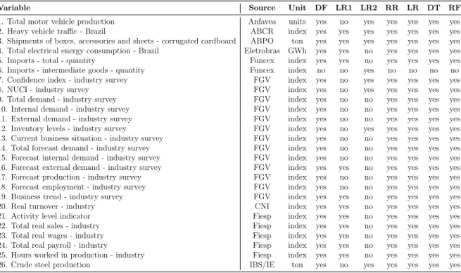
Details of the models estimated are given below. Apart from the SARIMA and structural models, which depend only on the provided time series, the remaining models require other variables for the estimates. The variables used are shown in Table 1 and were selected based on the literature review described in the Introduction. The models used were:
• SARIMA: the SARIMA model estimated is a SARIMA(2,1,2)(0,1,1)12. Two
dummies representing the months of Dec 2008 and Jan 2009 were inserted in the model. Details of the procedures for defining, estimating and validating this model can be found in Box & Jenkins (1970).
• Structural: the structural model breaks industrial production down into trend and seasonality, two of its non-observable components. A basic structural model was estimated (Durbin & Koopman, 2012). The components were estimated using a Kalman filter.
• Dynamic Factor: dynamic factor models summarize the information in many time series in only a few common (non-observable) factors. The variable of interest can then be forecasted using the factors based on the linear regression model. The methodology can handle missing values very well. These are often found at the end of the database series, because the explanatory variables are not all published at the same time. The dynamic factor model estimated here is explained nin more detail in Giannone et al. (2008) and Banbura et al. (2011) and can easily be replicated with the R nowcasting package (Mattos et al., 2018). The methodology, which uses a Kalman filter, can also forecast the explanatory variables, which are used in the regression and decision tree models described below.
• Regressions:
1. Linear regression (OLS): two linear regression models are estimated. One of these only uses variables that are considered coincident with the industrial production index. The other one considers only the variables that reduced the forecast error one-step-ahead in the last 48 months (stepwise regression). 2. Lasso and ridge regression: these are linear regression models with a penalty function that determines the size of the regression coefficients. One reason for using this type of model is that the resulting forecasts have smaller confidence intervals when many predictor variables are used. Each model has its own penalty function. In lasso regression, some coefficients can be exactly zero. Further details of the methodologies can be found in Tibshirani (1996). • Decision Tree: these are statistical methods that use supervised training to
forecast data. Further details can be found in Breiman et al. (1993); Breiman (2001). Here we estimate a regression tree and a random forest.
All the models were estimated using variables without any seasonal adjustment. To determine the month-over-month percentage change (i.e., the change at the margin), the forecasts were seasonally adjusted with X-13ARIMA-SEATS (U.S. Census Bureau, 2017) using the IBGE configurations in IBGE (2018). The year-over-year percentage change (interannual change) was calculated for the series without any seasonal adjust-ment. The forecasts shown here therefore refer to the series in levels (with/without seasonal adjustment), changes at the margin and year-over-year changes1.
1
The replication code for the results shown here can be found at https://github.com/nmecsys/ indprod, and the updated forecast for industrial production can be found at https://pedroferreira. shinyapps.io/indprod.
Variable Source Unit DF LR1 LR2 RR LR DT RF 1. Total motor vehicle production Anfavea units yes no yes yes yes yes yes 2. Heavy vehicle traffic - Brazil ABCR index yes yes yes yes yes yes yes 3. Shipments of boxes, accessories and sheets - corrugated cardboard ABPO ton yes yes yes yes yes yes yes 4. Total electrical energy consumption - Brazil Eletrobras GWh yes yes no yes yes yes yes 5. Imports - total - quantity Funcex index yes yes no yes yes yes yes 6. Imports - intermediate goods - quantity Funcex index no no yes no no no no 7. Confidence index - industry survey FGV index yes no yes yes yes yes yes 8. NUCI - industry survey FGV index yes no yes yes yes yes yes 9. Total demand - industry survey FGV index yes no no yes yes yes yes 10. Internal demand - industry survey FGV index yes no no yes yes yes yes 11. External demand - industry survey FGV index yes no no yes yes yes yes 12. Inventory levels - industry survey FGV index yes no yes yes yes yes yes 13. Current business situation - industry survey FGV index yes no no yes yes yes yes 14. Total forecast demand - industry survey FGV index yes no no yes yes yes yes 15. Forecast internal demand - industry survey FGV index yes no no yes yes yes yes 16. Forecast external demand - industry survey FGV index yes yes no yes yes yes yes 17. Forecast production - industry survey FGV index yes no no yes yes yes yes 18. Forecast employment - industry survey FGV index yes no no yes yes yes yes 19. Business trend - industry survey FGV index yes yes no yes yes yes yes 20. Real turnover - industry CNI index yes yes no yes yes yes yes 21. Activity level indicator Fiesp index yes yes no yes yes yes yes 22. Total real sales - industry Fiesp index yes yes no yes yes yes yes 23. Total real wages - industry Fiesp index yes yes no yes yes yes yes 24. Total real payroll - industry Fiesp index yes yes no yes yes yes yes 25. Hours worked in production - industry Fiesp index yes yes no yes yes yes yes 26. Crude steel production IBS/IE ton yes no yes yes yes yes yes DF: dynamic factor model; LR1: linear regression 1; LR2: linear regression 2; RR: ridge regression;
LR: lasso regression; DT: decision tree; RF: random forest
Table 1: Database - List of auxiliary variables
2.2
Forecast combination
Forecast combination involves combining two or more individual forecasts to produce a single forecast. The accuracy of the combined forecast is generally superior to that of the individual forecasts, and the use of simple combination methods such as mean and median, yield results on par with more sophisticated methods (Stock & Watson, 2006). The combined forecasts in the present paper were obtained in four different ways:
• mean: each forecast has the same weight in the combined forecast; • median: more robust to outliers;
• inverse error: weight defined by the inverse of the RMSE (root mean square error). Historical forecasts are needed to calculate the error;
• OLS: weights are defined by the coefficients of linear regression between the re-sponse variable and forecasts of these estimates without a constant. Historical forecasts are needed to estimate the regression.
3
Results
(pseudo out-of-sample) RMSEs statistics for each model discussed in section 2. The forecasts were made taking into account the last 48 months of industrial production.
inde x 70 80 90 100 110 2002 2004 2006 2008 2010 2012 2014 2016 2018 Level Level (SA)
Figure 1: Industrial production index - Jan 2002 to Jan 2018 (with and without seasonal adjustment)
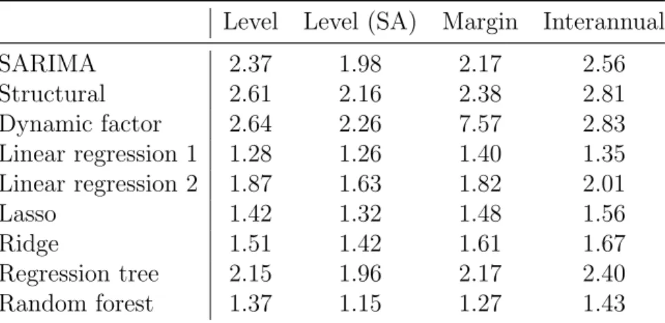
Level Level (SA) Margin Interannual
SARIMA 2.37 1.98 2.17 2.56 Structural 2.61 2.16 2.38 2.81 Dynamic factor 2.64 2.26 7.57 2.83 Linear regression 1 1.28 1.26 1.40 1.35 Linear regression 2 1.87 1.63 1.82 2.01 Lasso 1.42 1.32 1.48 1.56 Ridge 1.51 1.42 1.61 1.67 Regression tree 2.15 1.96 2.17 2.40 Random forest 1.37 1.15 1.27 1.43
Table 2: RMSE taking into account the last 48 months of one-step-ahead out-of-sample forecasts
The largest errors were produced by the univariate models (SARIMA and struc-tural) and the dynamic factor model. The univariate models were expected to have lower forecasting accuracy than the multivariate models. The poor performance of the dynamic factor model may be due to the small number of variables used to estimate the factors, as a result of which the information in the unobserved variable was insufficient.
The models with the smallest RMSEs were the linear regression and random forest mod-els with theses explanatory variables: heavy-vehicle traffic - Brazil (ABCR); shipment of boxes, accessories and sheets - corrugated cardboard (ABPO); total electrical energy consumption - Brazil (Eletrobras); imports - total (Funcex); forecast external demand and business trend (industry survey, FGV IBRE); real turnover - industry (CNI); and activity level indicator, total real sales, total real wages, total real payroll and hours worked in production (Fiesp, industry).
We estimated four types of forecasts combinations (section 2.2) to evaluate whether this strategy improves accuracy. Two types of combination (inverse error and OLS) need a prediction history to define the weight in the aggregation. So, we estimated the industrial production (one-step-ahead) for the last 48 months observed.
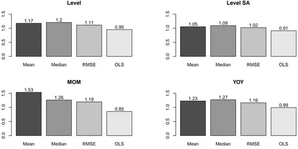
Mean Median RMSE OLS Level 0.0 0.5 1.0 1.5 1.17 1.2 1.11 0.95
Mean Median RMSE OLS Level SA 0.0 0.5 1.0 1.5 1.05 1.09 1.02 0.91
Mean Median RMSE OLS MOM 0.0 0.5 1.0 1.5 1.53 1.26 1.19 0.85
Mean Median RMSE OLS YOY 0.0 0.5 1.0 1.5 1.23 1.27 1.16 0.99
Figure 2: RMSE of one-step-ahead out-of-sample forecasts taking into account the last 48 months for each combination
Figure 2 shows the RMSE for the variable in levels with and without seasonal adjust-ment, margin and interannual rates. The errors for the combinations are significantly lower than those for any of the individual models (Table 2) apart from the error for the combination formed using the mean, which is greater (1.53) than the value for some models. The smallest error occurs when we use combination weights estimated by OLS.
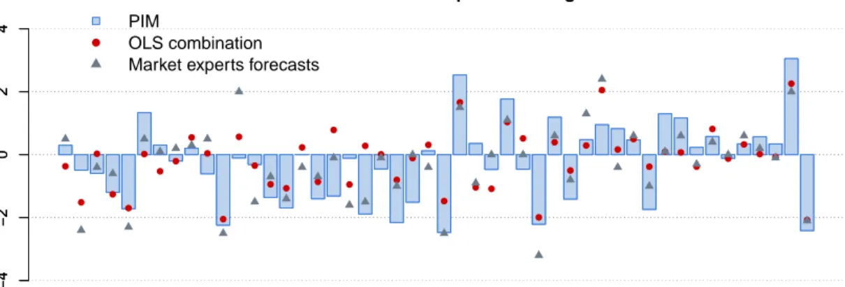
1 3 5 7 9 11 13 15 17 19 21 23 25 27 29 31 33 35 37 39 41 43 45 47 −4 −2 0 2 4
month−over−month percent change
−4 −2 0 2 4 PIM OLS combination Market experts forecasts
(a) Forecast variation at the margin
1 3 5 7 9 11 13 15 17 19 21 23 25 27 29 31 33 35 37 39 41 43 45 47 −15 −10 −5 0 5 10
year−over−year percent change
−15 −10 −5 0 5 10 PIM OLS combination Market experts forecasts
(b) Forecast year-over-year variation
Figure 3: Comparison of one-step-ahead market and OLS combination forecasts for the last 48 months observed.
Figure 3 shows, in addition to the OLS combination forecast, the median of the market experts forecast (Bloomberg) for industrial production in the last 48 months of the period analyzed. The blue bars correspond to the observed value of industrial production, the red dots are the estimated values using the OLS combination and the gray triangles to the market experts forecasts, the median of forecasts made by various specialists.
Overall, our estimates are better than the median of the market experts forecasts, indicating that the technique used here can rival market expert forecasts. The RMSEs for the OLS combination and market experts forecasts are, respectively, 0.99 and 1.12
on a year-over-year basis, and 0.85 and 0.86 for month-over-month rate for the period observed. Here, it’s necessary to call attention to the following points: (i) taking into account yoy comparison, the forecasts accuracy were improved nearly 10% and (ii) most of market experts results are released just two days before official estimate is released. In other words, our error measure is lower and we can release our estimates one month before.
4
Final considerations
This study sought to develop a model for forecasting industrial production in Brazil. A variety of methods for forecasting it have been developed because of the importance of this variable when analyzing the economic scenario. Here, we estimated SARIMA model, linear regressions (dynamic, ridge and lasso), structural and dynamic factor models and decisions trees. The techniques that produced the smallest out-of-sample one-step-ahead forecast error were the random forest method and a linear regression model.
Combination forecasting using all the models proved satisfactory as it resulted in a considerable reduction in forecast error and its performance was superior to that of the best models estimated here. For the month-over-month variation, for example, the RMSE, which varied between 1.27 and 7.57 for the individual models, was reduced to 0.85 for one of the combinations. The most effective combination, among the four evaluated, was the combination based on a linear regression model (OLS).
Our forecast strategy proved competitive with the median of forecasts by various specialists as we have lower errors and we disclosed it more quickness.
References
Banbura, M., Giannone, D., & Reichlin, L. (2011). Nowcasting. Oxford Handbook on Economic Forecasting.
Bazzi, M., Blasques, F., Koopman, S. J., & Lucas, A. (2017). Time-varying transition probabilities for markov regime switching models. Journal of Time Series Analysis, 38 (3), 458–478. 10.1111/jtsa.12211.
URL http://dx.doi.org/10.1111/jtsa.12211
Berge, T. J. (2015). Predicting recessions with leading indicators: Model averaging and selection over the business cycle. Journal of Forecasting, 34 (6), 455–471. For.2345. URL http://dx.doi.org/10.1002/for.2345
Bodo, G., Golinelli, R., & Parigi, G. (2000). Forecasting industrial production in the euro area. Empirical Economics, 25 (4), 541–561.
Box, G. E. P., & Jenkins, G. M. (1970). Time Series Analysis forecasting and control . San Francisco: Holden Day.
Breiman, L. (2001). Random forests. Machine Learning, 45 (1), 5–32. URL https://doi.org/10.1023/A:1010933404324
Breiman, L., Friedman, J., Olshen, R. A., & Stone, C. J. (1993). Classification and regression trees. wadsworth, 1984. Google Scholar .
Bulligan, G., Golinelli, R., & Parigi, G. (2010). Forecasting monthly industrial produc-tion in real-time: from single equaproduc-tions to factor-based models. Empirical Economics, 39 (2), 303–336.
URL http://dx.doi.org/10.1007/s00181-009-0305-7
Costantini, M. (2013). Forecasting the industrial production using alternative factor models and business survey data. Journal of Applied Statistics, 40 (10), 2275–2289. Durbin, J., & Koopman, S. J. (2012). Time Series Analysis by State Space Methods.
Oxford University Press, 2 ed.
Elliott, G., Granger, C., & Timmerman, A. (2006). Macroeconomic forecasting using many predictors (with james h. stock). Handbook of Economic Forecasting.
Giannone, D., Reichlin, L., & Small, D. (2008). Nowcasting: The real-time infor-mational content of macroeconomic data. Journal of Monetary Economics, 55 (4), 665–676.
Hassani, H., Heravi, S., & Zhigljavsky, A. (2013). Forecasting uk industrial production with multivariate singular spectrum analysis. Journal of Forecasting, 32 (5), 395–408. Hollauer, G., Issler, J. V., & Notini, H. H. (2008). Prevendo o crescimento da produ¸c˜ao industrial usando um n´umero limitado de combina¸c˜oes de previs˜oes. Economia Apli-cada, 12 , 177 – 198.
IBGE (2018). Pesquisa industrial mensal - produ¸c˜ao f´ısica, notas metodol´ogicas.
URL http://www.ibge.gov.br/home/estatistica/indicadores/industria/
pimpf/br/notas_metodologicas.shtm
Madsen, J. B. (1993). The predictive value of production expectations in manufacturing industry. Journal of Forecasting, 12 (3-4), 273–289.
Mattos, D., Branco Gomes, G., & Costa Ferreira, P. (2018). nowcasting: Nowcast Analysis and Create Real-Time Data Basis. R package version 0.1.3.
URL https://github.com/nmecsys/nowcasting
Seong, B., Ahn, S. K., & Zadrozny, P. A. (2013). Estimation of vector error correction models with mixed-frequency data. Journal of Time Series Analysis, 34 (2), 194–205. URL http://dx.doi.org/10.1111/jtsa.12001
Stock, J. H., & Watson, M. (2006). Forecasting with many predictors. vol. 1, chap. 10, (pp. 515–554). Elsevier, 1 ed.
URL https://EconPapers.repec.org/RePEc:eee:ecofch:1-10
Thury, G., & Witt, S. F. (1998). Forecasting industrial production using structural time series models. Omega, 26 (6), 751 – 767.
URL http://www.sciencedirect.com/science/article/pii/
S0305048398000243
Tibshirani, R. (1996). Regression shrinkage and selection via the lasso. Journal of the Royal Statistical Society. Series B (Methodological), 58 (1), 267–288.
URL http://www.jstor.org/stable/2346178
U.S. Census Bureau (2017). X-13ARIMA-SEATS Reference Manual Acessible HTML Output Version.
URL https://www.census.gov/ts/x13as/docX13AS.pdf
Vasnev, A., Skirtun, M., & Pauwels, L. (2013). Forecasting monetary policy decisions in australia: A forecast combinations approach. Journal of Forecasting, 32 (2), 151– 166.